Automatic BIM Reconstruction for Existing Building MEP Systems from Drawing Recognition

Abstract

Aging buildings pose a significant concern for many large developed cities, and the operation and maintenance (O&M) of mechanical, electrical, and plumbing (MEP) systems becomes critical. Building Information Modeling (BIM) facilitates efficient O&M for MEP. However, these numerous aging buildings were constructed without BIM, making BIM reconstruction a monumental undertaking. This research proposes an automatic approach for generating BIM based on 2D drawings. Semantic segmentation was utilized to identify MEP components in the drawings, trained on a custom-made MEP dataset, achieving an mIoU of 92.18%. Coordinates and dimensions of components were extracted through contour detection and bounding box detection, with pixel-level accuracy. To ensure that the generated components in BIM strictly adhere to the specifications outlined in the drawings, all model types were predefined in Revit by loading families, and an MEP component dictionary was built to match dimensions and model types. This research aims to automatically and efficiently generate BIM for MEP systems from 2D drawings, significantly reducing labor requirements and demonstrating broad application potential in the large-scale O&M of numerous aging buildings.

1. Introduction

As the urbanization process in many large developed cities enters the stage of stock renewal, the operation and maintenance (O&M) of existing buildings has become an important issue in the construction industry [1]. In numerous existing buildings, the Mechanical, Electrical, and Plumbing (MEP) systems exhibit varying degrees of aging [2], with issues such as reduced energy efficiency of HVAC (Heating, Ventilation, and Air Conditioning) equipment, leaks in the water supply and drainage systems, and aging electrical wiring being particularly prominent. These problems not only affect the functionality of the building but also pose safety risks [3].

Traditional MEP system O&M methods mainly rely on paper documentation, such as manually consulting as-built drawings and maintenance records. This leads to fragmented information storage and inefficient retrieval, and delays in document updates prevent it from accurately reflecting the current condition of the building [4]. With the increasing number of aging buildings, the workload involved in MEP system O&M cannot be underestimated. Inefficient traditional O&M methods result in increased waste of manpower, time, and financial resources, highlighting the urgent need for an efficient O&M approach. BIM has significantly improved the efficiency of MEP system O&M in various ways [5]. BIM provides an intuitive 3D model, helping O&M staff to better understand the layout of the MEP systems, thereby reducing misunderstandings caused by 2D drawings. At the same time, BIM includes detailed equipment data, specifications, and historical records, enabling O&M staff to quickly access the necessary information, thus avoiding the cumbersome manual process of document consultation. Specifically, by analyzing historical data and operational conditions through BIM, potential issues can be predicted in advance, allowing for preventive maintenance to be scheduled and reducing the occurrence of unexpected failures.

However, BIM began to be widely adopted globally only in 2012 [6], and many aging buildings, due to their older construction dates, have not yet been equipped with BIM models. Traditional methods for generating BIM rely heavily on manual operations, which are time-consuming, labor-intensive, and prone to errors [7]. Therefore, to address the MEP system O&M needs of a large number of aging buildings, an efficient, automated method is required to generate BIM models for these buildings.

Substantial studies on automatic BIM generation mainly utilized two types of data sources, point cloud and 2D drawings (CAD files and raster drawings).

The advent of modern technologies such as 3D-LiDAR scanning and depth camera photography has facilitated the generation of point clouds [8]. The typical process for BIM generation based on point clouds is scan-to-BIM. Dimotrov et al. [9] generated BIM by utilizing 3D laser scanning to capture the point cloud of buildings and subsequently creating BIM models of these structures. Wang et al. [10] integrated scanned point clouds with RGB images collected by depth cameras, employed pre-trained visual networks to identify MEP components, and converted 2D labels into corresponding 3D point cloud data to provide precise geometric information for the establishment of BIM. Despite the capability of point cloud scanning to produce highly accurate BIM models, acquiring point clouds necessitates fieldwork, which remains labor-intensive and time-consuming. Furthermore, it is challenging to obtain point cloud data hidden within walls, ceilings, or floors [11].

Generating BIM for building projects based on 2D drawings is an economical and efficient approach. When CAD files are available, Park et al. [12] proposed an automated process for generating BIM of ducts by leveraging layer information within CAD files and utilizing Dynamo for modeling, which shortened the time required for ductwork BIM generation. Cho et al. [13] analyzed the content and characteristics of mechanical components represented in various drawings in DXF format and developed a classification and algorithm that supports the automatic recognition of the spatial information data of mechanical systems. However, CAD only became popular in the late 1990s [14], meaning that buildings older than 30 years lack the CAD systems necessary to generate BIM. These aging buildings, which are particularly problematic for MEP system O&M, require a method that uses scanned images of paper drawings as the basis for BIM generation.

Currently, with the rapid advancement of deep learning in the field of computer vision, significant achievements have been made in the application of image recognition in areas such as medicine, remote sensing, and materials science [15,16]. It has also demonstrated great potential in engineering drawing recognition [17]. There have been successful studies on generating BIM from 2D drawings using visual recognition. Zhao et al. [18] proposed a hybrid method for generating BIM from 2D structural floor plans, integrating techniques such as image processing, deep learning, and Optical Character Recognition (OCR). The method extracts information about grids, columns, and beams from the image of the structural drawing and generates a BIM model of the structure. Pan et al. [19] introduced a methodology to extract information from 2D MEP drawings and reconstruct BIM models. Semantic information is extracted through image cropping and instance segmentation, while geometric information is obtained via semantic-assisted image processing. Finally, BIM models are reconstructed using Industry Foundation Classes (IFCs) based on the geometric information.

In object recognition, recent studies utilize deep learning, such as object detection, semantic segmentation, and instance segmentation. These methods use neural networks to extract features of components and classify them. Object detection performs well on divisible objects but performs poorly on continuous linear objects such as ducts [20]. Semantic segmentation has better recognition performance for continuous linear objects and can capture the outer contours of irregular objects, but its disadvantage is that it cannot distinguish between different instances [21]. Instance segmentation can detect the outer contour of an object and generate bounding boxes, but, due to insufficient geometric information, the detected contour does not fully match the actual shape, resulting in rough boundaries [22].

In geometric shape extraction, recent studies employ methods such as computer vision, predefined recognition, and annotation analysis to identify the contours and dimensions of objects. Computer vision techniques can accurately detect the pixel regions and contours of geometric objects. For example, contour detection [23] can extract the contours of images, find the maximum gradient in the image to detect edges, and improve the accuracy and stability of detection results through non-maximum suppression and double thresholding. Predefined recognition [24] uses predetermined patterns or patterns to detect the position and size of objects with specific shapes. This method works well for objects with obvious features but is sensitive to object rotation. Annotation recognition [25] uses annotations to obtain the dimensions of components, which performs well on objects with simple geometric shapes such as beams, slabs, and columns in structural diagrams. However, MEP components are often irregularly shaped, making it difficult for this method to accurately determine the shape of such irregular objects.

In coordinate extraction, recent studies use methods such as direct extraction, semantic-assisted contour extraction, and semantic-assisted skeleton extraction. The direct extraction method [26] utilizes semantic segmentation results to traverse the image to find all pixels belonging to the target class and record their coordinates. However, these coordinates are massive and cannot determine the key coordinates required for constructing a BIM. Semantic-assisted contour detection [27] is a method that combines instance segmentation results and connected domain analysis to accurately obtain irregular component contours by merging similar bounding boxes and masks, labeling connected domains, and filtering overlapping pixel ratios. However, the ducts in MEP images are complex and intricate, which can result in multiple ducts being within the same bounding box. The direction of the generated bounding box is also single, making it unsuitable for MEP components with rotation angles. The semantic-assisted skeleton extraction method [28] extracts the centerline of the component based on the mask contour of the line type component. However, the mask contour is rough, and the coordinates of the two endpoints of the detected centerline are inaccurate.

Through the literature review, it has been found that there are still shortcomings in extracting information based on 2D drawing recognition for BIM generation:

• The components of MEP systems must work in coordination and have strong interdependence, which imposes strict requirements on coordinate accuracy in modeling. However, the coordinate detection accuracy in current studies often fails to meet the requirements of construction specifications;
• MEP components come in various classes, each containing types of different sizes. BIM models generated from semantic segmentation masks in recent studies have met the requirements for planar geometric shapes. But their dimensions overlook the equipment specifications provided in the drawings and design modulus, as well as the height of the components along the Z-axis.

This research aims to recognize drawings in order to generate BIM with both accurate coordinates and dimensions, using the following innovative methods:

• Semantic segmentation is used to identify MEP components in the drawings and extract their semantic information, with a custom-made MEP dataset used to train the neural network beforehand;
• Key coordinates and dimensions of MEP components are extracted through contour detection and bounding box detection. For duct components, OCR-based annotation recognition is specifically used to identify the height on the Z-axis;
• All model types in Revit are predefined, and an MEP component dictionary is built, ensuring that all generated BIM models comply with the specifications.

2. Methods

This research proposes a hybrid approach that utilizes semantic segmentation combined with computer vision techniques to identify and extract parameters such as the class, coordinates, and pixel count of components from MEP 2D drawings. Specifically, for duct components, OCR annotation recognition is additionally applied to obtain the height on the Z-axis. The pixel count or annotations are then matched to the pre-built MEP component dictionary to identify the specific model type of the component. Finally, Dynamo is used to automatically generate the Revit model of the MEP components based on the extracted coordinates and the model dimensions matched from the dictionary.

The phases are as follows and presented in Figure 1.

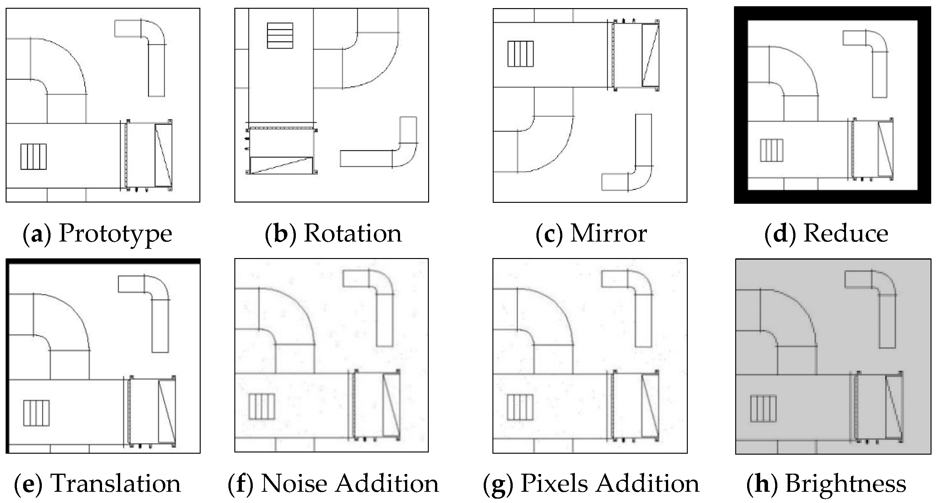
• Creation of the MEP Dataset: First, identify the classes of components that need to be recognized and collect data images. Subsequently, use a sliding window to crop the data images, annotate the images using Labelme, and perform data augmentation. This step ensures that the dataset is diverse and robust, enhancing the training process for the recognition network. The augmented data is then ready for use in training the deep learning network, ensuring better generalization and accuracy when applied to real-world MEP 2D drawings;
• Semantic Segmentation Training and Prediction: Use MMSegmentation to train several neural networks on the MEP dataset. The best network which achieves the highest evaluating indicator (mIoU) is then utilized to predict images. Next, apply sliding window cropping to break the MEP drawing of a certain floor into smaller cropped images and predict them. Finally, use sliding window stitching to combine the predicted masks from the cropped images into a complete mask image of the entire floor;
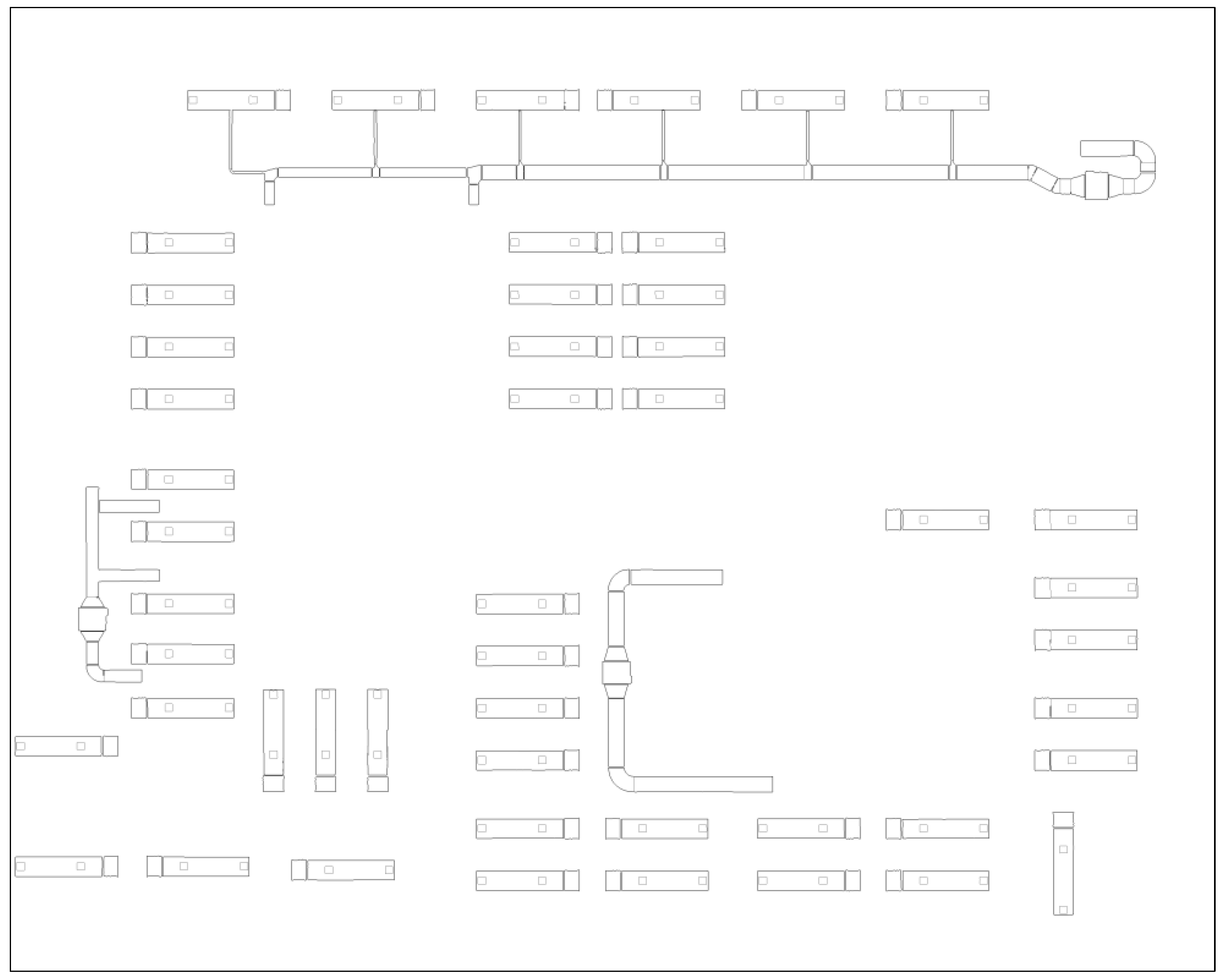
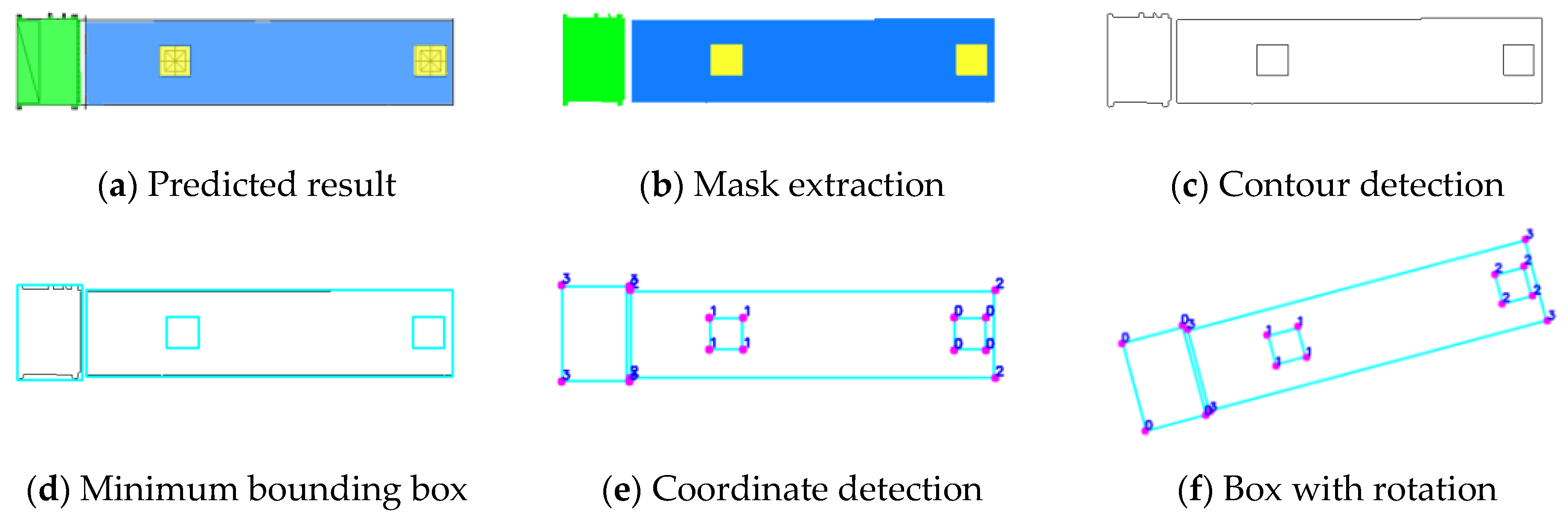
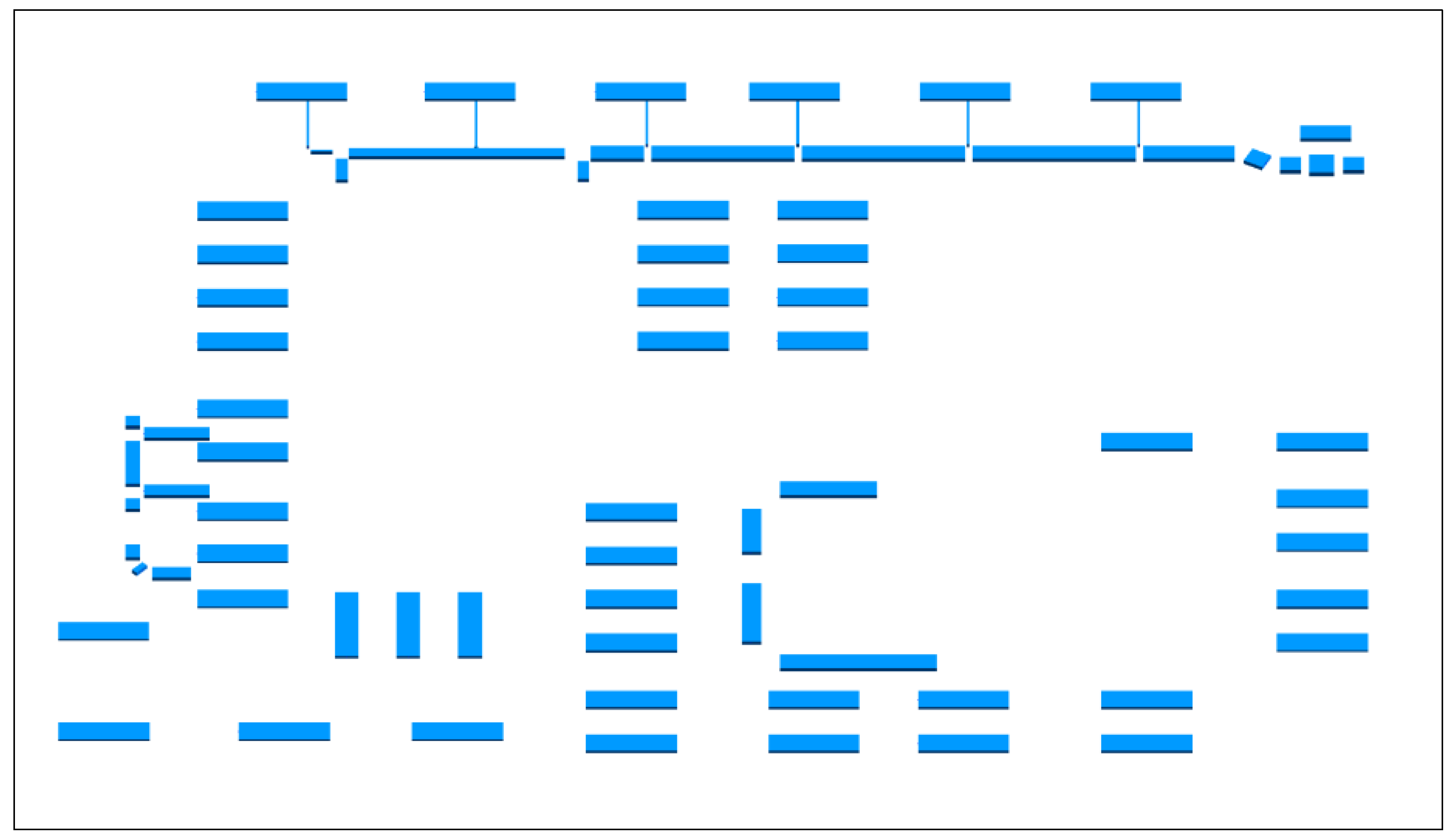
• Contour and Bounding Box Detection: Perform contour detection on the complete mask image to obtain the contours of each component and generate an overall contour image. Then, separate the overall contour image into several individual images. For each component contour in each separated image, generate the minimum bounding rectangular box with a rotation angle;
• Coordinate Transformation and Type Matching: In terms of coordinate transformation, the key point coordinates for modeling, such as the center point and rotation angle for equipment or the two endpoints for ducts, are obtained based on the four corner coordinates extracted from the bounding box. In terms of type matching, an MEP component dictionary is used to match the extracted dimensions with the specifications. For the equipment component, the coordinates of the bounding box are applied to the mask image, and the number of pixels within the component mask inside the bounding box is counted. The pixel count is then converted to the actual size to match the specific model in the dictionary. For the ducts component, OCR is utilized to recognize annotation. Firstly, the annotation is matched with the component based on coordinates, and then the specific model in the dictionary is matched based on the text content;
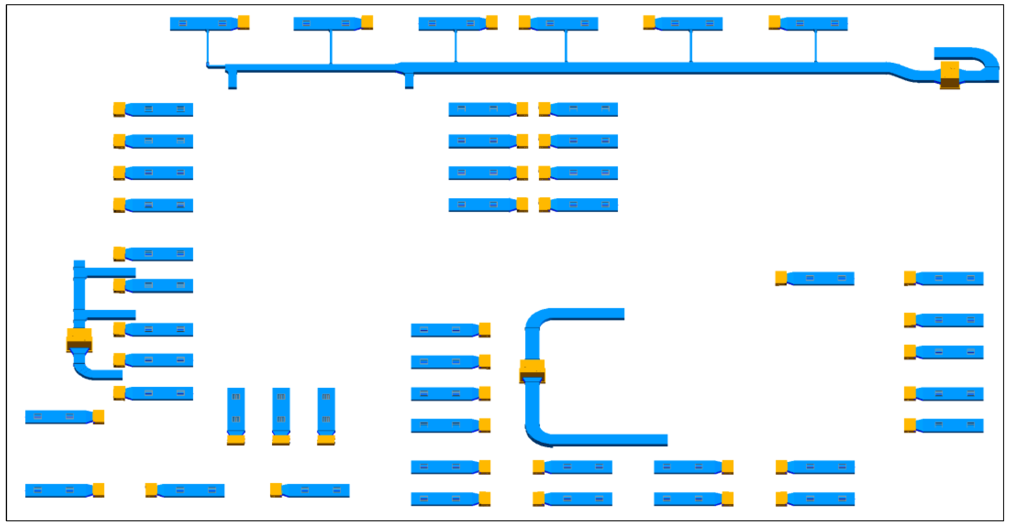
• Automatic BIM Generation: Write the coordinates and dimensions required for modeling into Excel and use Dynamo to generate 3D models.

2.1. Semantic Segmentation of 2D Drawings

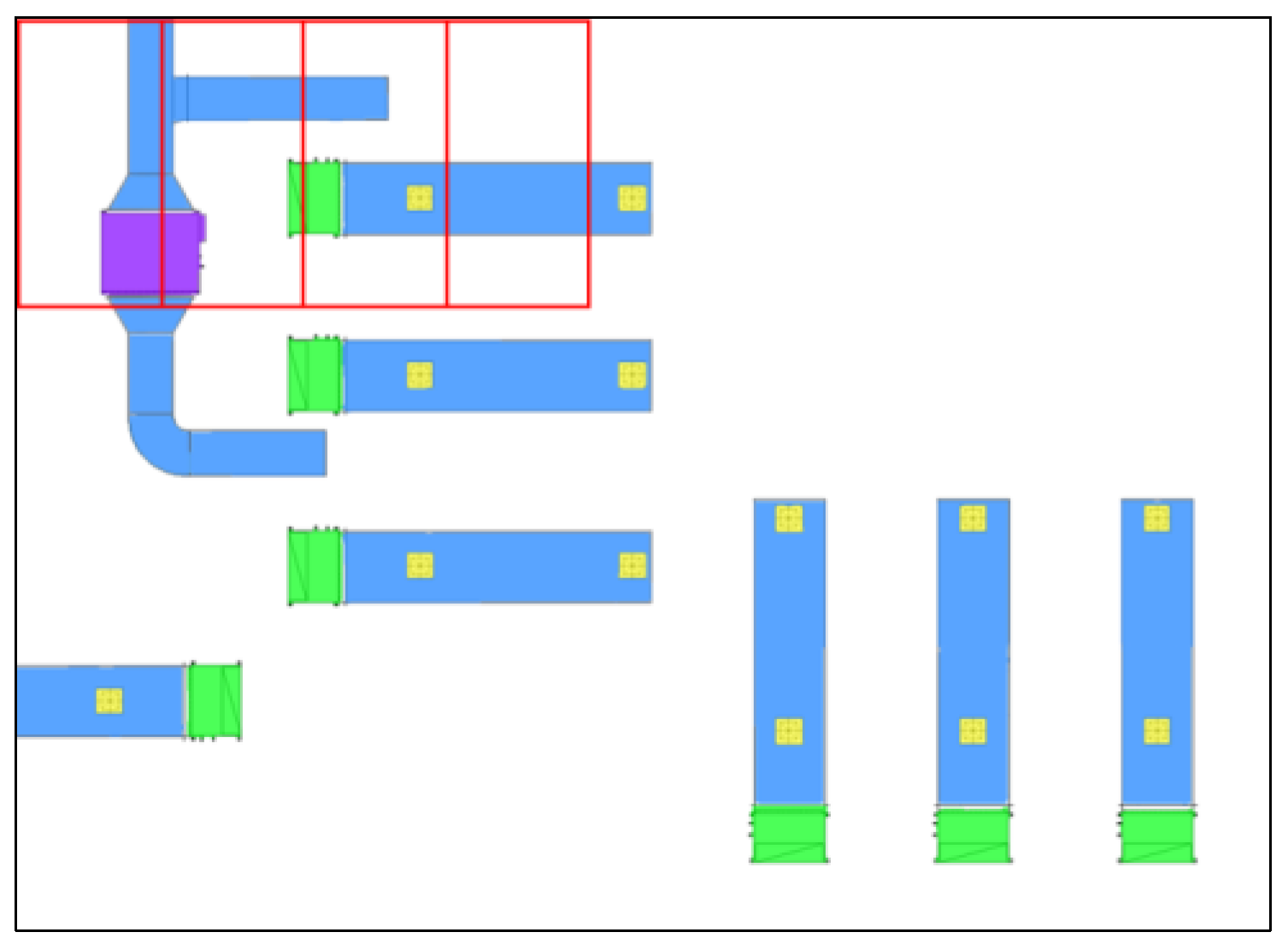
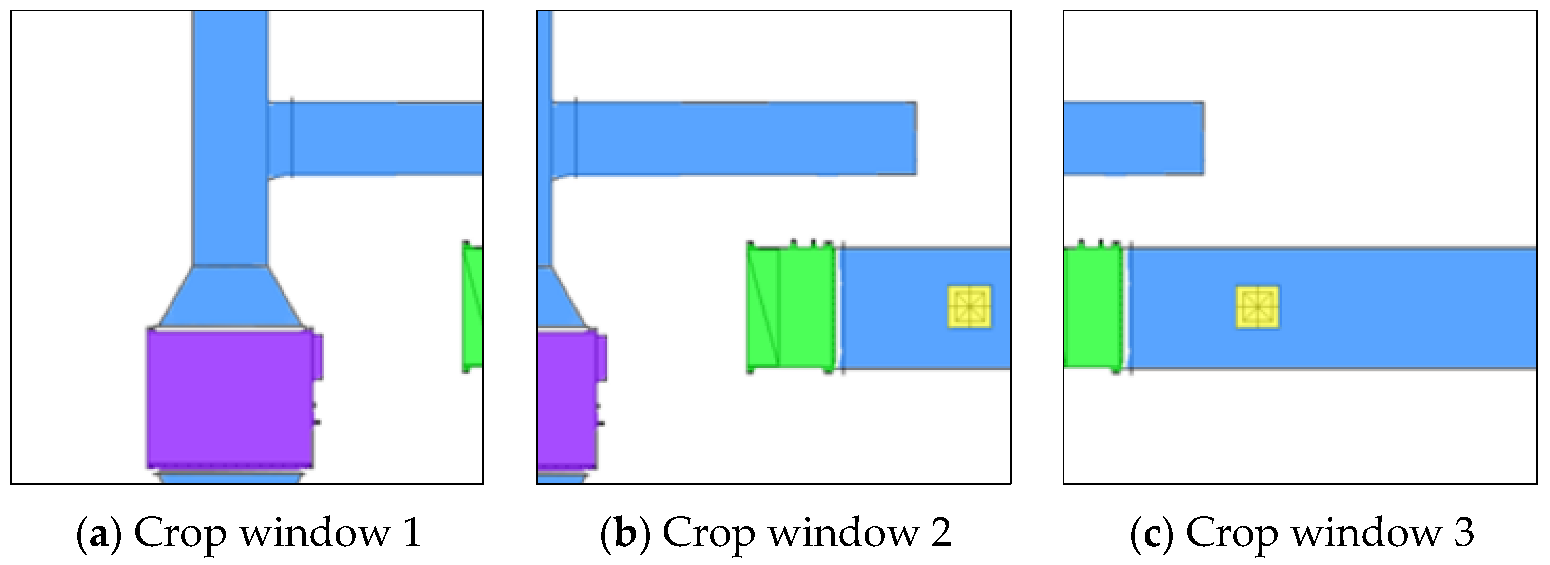
2.1.1. Sliding Window Cropping for Multi-Scale Component Recognition

To predict the MEP drawings of a certain floor, some small-sized components in the overall image cannot be recognized due to their small proportion within the image. Additionally, the large-scale and high-resolution nature of the image poses challenges for both computer performance and neural networks [29]. Consequently, the large-sized image is segmented into smaller ones by means of window-based image cropping, as depicted in Figure 2. During this process, the image area within each window is processed separately, which enlarges the proportion of components [30], makes the characteristics of components more prominent, and leads to better prediction results, as depicted in Figure 3. Moreover, if the same component is cropped into multiple images, a portion of the component in a single cropped image may become unrecognizable due to its indistinct characteristics, in this research, a fixed-size window slides over the entire image, analyzing the image’s local features block by block. A specific step length is set when sliding, ensuring the entire image is covered. The window size is chosen to both encompass the characteristics of components and maintain an appropriate resolution.

2.1.2. MMSegmentation for Semantic Segmentation

MMSegmentation is a semantic segmentation network library based on PyTorch, provided by the OpenMMLab open-source project. It integrates numerous high-quality semantic segmentation networks, such as DeepLabV3+, K-Net, and Segfozrmer. With its unified framework, flexible module design, and concise training and inference interfaces, users can easily perform training, evaluation, and prediction for different networks through configuration files and make fair performance comparisons.

To obtain the semantic information of MEP components in images, this research utilized the MMSegmentation semantic segmentation network library and invoked multiple neural network architectures for training. During the training process, for each neural network, the weight configurations that performed best on the specified evaluation metrics were retained. Subsequently, the network with the optimal evaluation metrics was selected from these screened weights for image prediction.

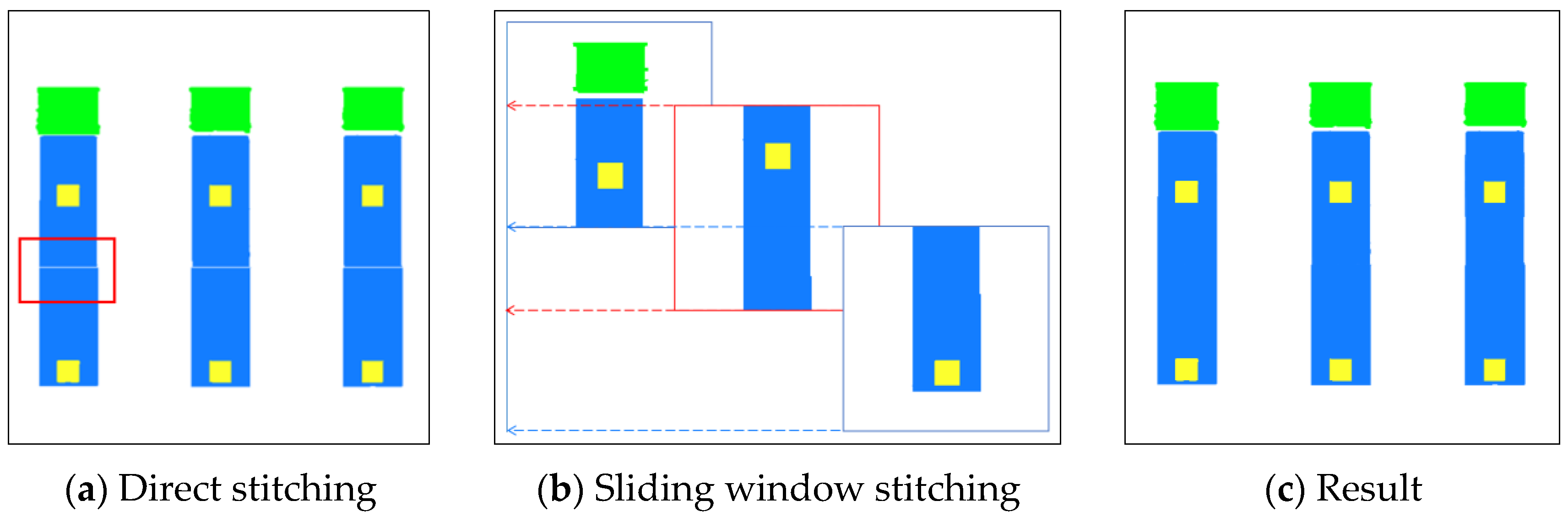
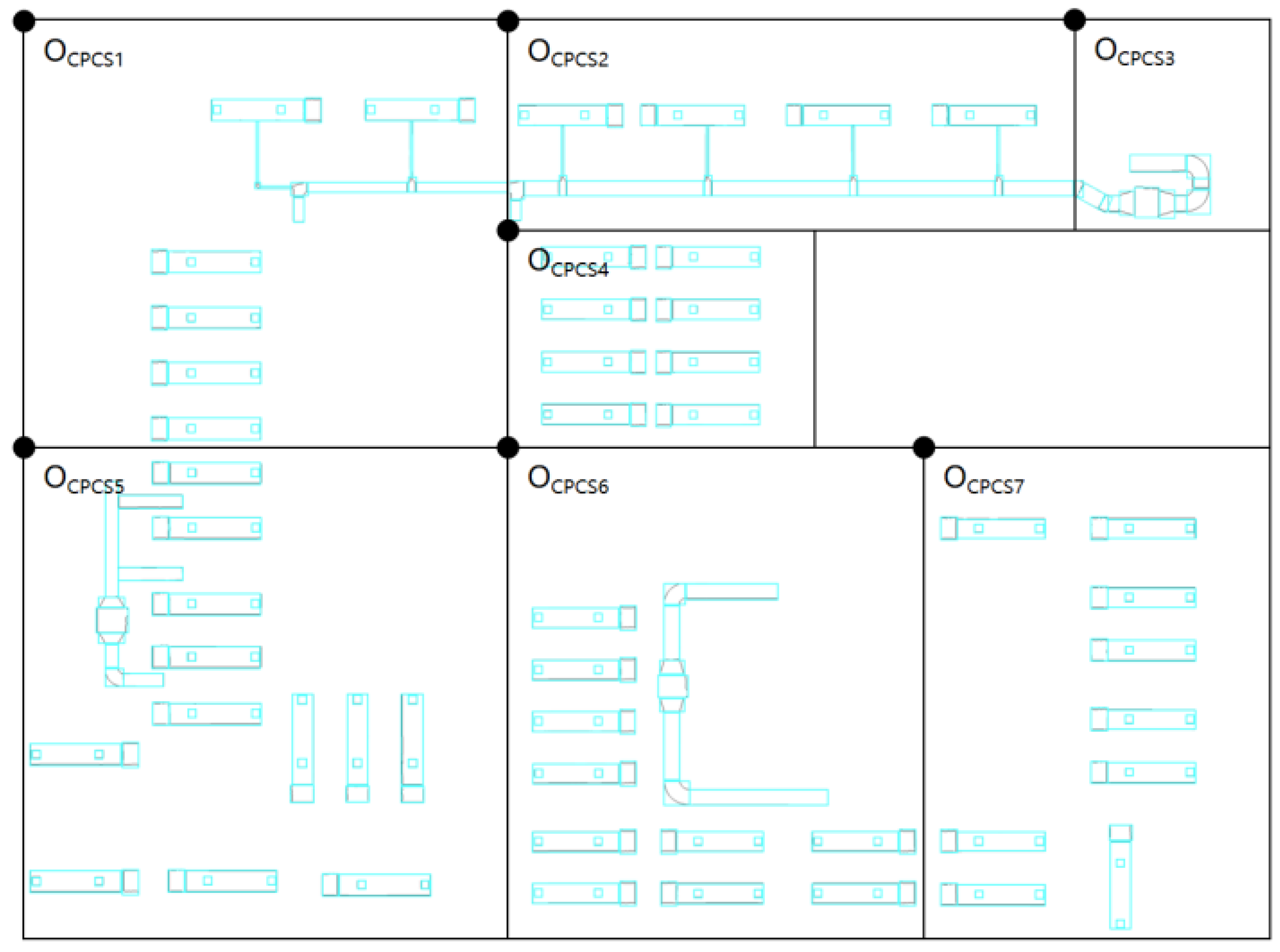
2.1.3. Sliding Window Stitching for a Overall Mask Image

After obtaining the mask for each cropped image through prediction, since a single cropped image cannot fully represent all the contents of MEP components, the components may only appear partially due to cropping. Therefore, it is necessary to stitch the cropped images together to form the overall MEP image of the floor, so that all components can be presented simultaneously on the same high-resolution overall image. However, if the method of non-overlapping image stitching is utilized, obvious gaps may appear at the junctions of the images when stitching the images, as shown in Figure 4a.

Consequently, before prediction, it is required to perform sliding window cropping on the MEP drawings, and each cropped image was predicted individually. After prediction, the mask images from each cropped image are stitched into an overall mask image through the sliding window stitching method, eliminating any impact on subsequent processes. The overall MEP mask of a certain floor is shown in Figure 5.

2.2. Extraction and Transformation of Coordinates

2.2.1. Coordinate Extraction

In the mask images obtained from semantic segmentation prediction, the geometric shapes of equipment are complex and there are a vast number of pixel coordinates. However, only a few key coordinates are needed during model generation. Therefore, it is necessary to simplify the mask images from semantic segmentation to reduce the complexity of data processing and improve the efficiency of coordinate detection.

Contour detection helps to identify the contours and shapes of objects in an image, enabling object detection and segmentation [31]. After obtaining the overall mask image of a certain floor, contour detection is utilized to extract the boundaries of targets and identify and locate the targets.

Gaussian–Laplacian detection [32] can clearly distinguish various multi-scale and irregular color patches and generate simple and clear closed contours, which demonstrates great applicability in this research. When performing Laplacian contour detection, if the image is not smoothed, it will respond significantly to noise. Therefore, the image is typically first subjected to Gaussian smoothing to suppress noise, and then Laplacian contour detection is carried out to highlight the edges. However, this method involves two independent convolution operations, which increases the computational complexity. To optimize this process, the Laplacian transformation is performed using the two-dimensional Gaussian function to control the number of convolutions to one. Equations (1) and (2) show the calculation process of this transformation. The detection results are shown in Figure 6.

$$\mathrm{g}\mathrm{a}\mathrm{u}\mathrm{s}\mathrm{s}\left(\mathrm{x},\mathrm{y},\mathrm{\sigma }\right)={\displaystyle \frac{1}{2\mathrm{\pi }{\mathrm{\sigma }}^2}}\mathrm{e}\mathrm{x}\mathrm{p}\left(-{\displaystyle \frac{{\mathrm{x}}^2+{\mathrm{y}}^2}{2{\mathrm{\sigma }}^2}}\right)$$

(1)

$$\begin{array}{cc}\left(\mathrm{g}\mathrm{a}\mathrm{u}\mathrm{s}\mathrm{s}\left(\mathrm{x},\mathrm{y},\mathrm{\sigma }\right)\right)& ={\displaystyle \frac{{\nabla }^2\left(\mathrm{g}\mathrm{a}\mathrm{u}\mathrm{s}\mathrm{s}\left(\mathrm{x},\mathrm{y},\mathrm{\sigma }\right)\right)}{{\partial x}^2}}+{\displaystyle \frac{{\nabla }^2\left(\mathrm{g}\mathrm{a}\mathrm{u}\mathrm{s}\mathrm{s}\left(\mathrm{x},\mathrm{y},\mathrm{\sigma }\right)\right)}{{\partial y}^2}}\hfill \\ & ={\displaystyle \frac{1}{2\mathrm{\pi }{\mathrm{\sigma }}^2}}{\displaystyle \frac{\partial \left(-\frac{x}{{\mathrm{\sigma }}^2}exp\left(-\frac{{\mathrm{x}}^2+{\mathrm{y}}^2}{2{\mathrm{\sigma }}^2}\right)\right)}{\partial x}}+{\displaystyle \frac{1}{2\mathrm{\pi }{\mathrm{\sigma }}^2}}{\displaystyle \frac{\partial \left(-\frac{x}{{\mathrm{\sigma }}^2}exp\left(-\frac{{\mathrm{x}}^2+{\mathrm{y}}^2}{2{\mathrm{\sigma }}^2}\right)\right)}{\partial y}}\hfill \\ & ={\displaystyle \frac{1}{2\mathrm{\pi }{\mathrm{\sigma }}^4}}\left({\displaystyle \frac{{\mathrm{x}}^2}{{\mathrm{\sigma }}^2}}-1\right)\mathrm{e}\mathrm{x}\mathrm{p}\left(-{\displaystyle \frac{{\mathrm{x}}^2+{\mathrm{y}}^2}{2{\mathrm{\sigma }}^2}}\right)+{\displaystyle \frac{1}{2\mathrm{\pi }{\mathrm{\sigma }}^4}}\left({\displaystyle \frac{{\mathrm{y}}^2}{{\mathrm{\sigma }}^2}}-1\right)\mathrm{e}\mathrm{x}\mathrm{p}\left(-{\displaystyle \frac{{\mathrm{x}}^2+{\mathrm{y}}^2}{2{\mathrm{\sigma }}^2}}\right)\hfill \\ & ={\displaystyle \frac{1}{2\mathrm{\pi }{\mathrm{\sigma }}^4}}\left({\displaystyle \frac{{\mathrm{x}}^2+{\mathrm{y}}^2}{{\mathrm{\sigma }}^2}}-1\right)\mathrm{e}\mathrm{x}\mathrm{p}\left(-{\displaystyle \frac{{\mathrm{x}}^2+{\mathrm{y}}^2}{2{\mathrm{\sigma }}^2}}\right)\hfill \end{array}$$

(2)

After the Gaussian–Laplacian contour detection, the minimum bounding box detection is performed for each closed line segment. The coordinates of the four corner points of each bounding box are extracted, and the key coordinates required for modeling are calculated based on these four corner points. For equipment components, the coordinates of the center point and the rotation angle are needed, while, for air ducts, only the coordinates of the two endpoints of the centerline are required.

After the mask image undergoes contour detection, the ‘cv2.findContours’ function is utilized to find all the contours and their hierarchical structures in the binary image. Set ‘cv2.RETR_TREE’ to obtain the complete hierarchical structure of the contours. Traverse each of the found contours, and use the ‘cv2.minAreaRect’ function to calculate the minimum bounding box for each contour. When the bounding box is generated, it surrounds the contour by rotation to obtain the bounding box with the minimum area. Finally, use ‘cv2.boxPoints’ to extract the vertex coordinates of these bounding boxes. Traverse all the contours, and, at the same time, define a ‘contour_id’ to assign a unique ID to each contour. Then, use ‘pandas’ to write the contour ID and its corresponding corner point coordinates into an Excel file, so as to facilitate the subsequent processing and analysis of the data. The detailed procedure is depicted in Figure 7.

2.2.2. Image Cropping and Coordinate Transformation

Due to the current limitations of computer and algorithm performance, errors may occur in the results obtained when performing the minimum bounding box detection on the overall contour image of the floor. Therefore, it is necessary to crop the overall contour image to reduce the number of closed curves in a single cropped image and improve the accuracy of the minimum bounding box detection. At this time, during the cropping process, an appropriate window size can be selected according to the size, position, and other conditions of the contour lines, and the windows do not need to be overlapped. During the cropping process, the pixel coordinates of the origin of each cropped image on the overall image (O_CPCSi) are recorded. Figure 8 shows the generation of the minimum bounding boxes after partitioning the overall contour detection image of the floor.

After extracting the pixel coordinates from the partitioned images, coordinate transformation is required to obtain the coordinates needed for modeling. The transformation process of a key point coordinate is divided into four steps:

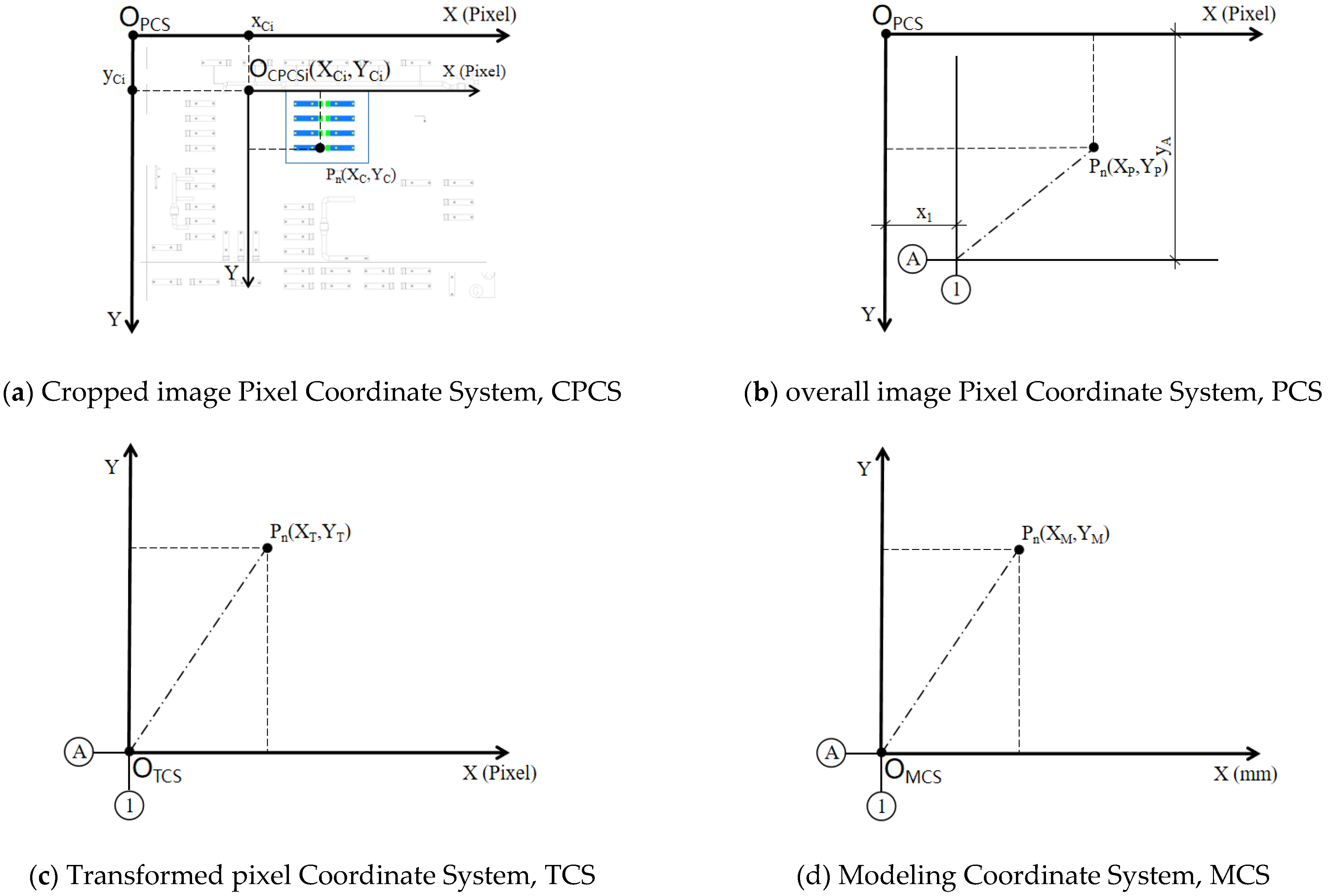
• Establish the CPCS (Cropped image Pixel Coordinate System) and the PCS (overall image Pixel Coordinate System). Record the coordinate of the cropped image origin (O_CPCSi) in the PCS. Extract the P_n(X_C, Y_C) in the CPCS and transform it to (X_P, Y_P) in PCS, as in Equation (3).
• In the PCS, identify and extract the pixel length of x₁ of the leftmost vertical axis line and the pixel length of y_A for the ordinate of the bottommost horizontal axis line (x₁, y_A are shown in Figure 9b).
• Establish the TCS (Transformed pixel Coordinate System). Transform the pixel abscissa and ordinate to obtain P_n(X_T, Y_T). Perform translation transformation on the abscissa and inversion transformation on the ordinate, as in Equation (4).
• Establish the MCS (Modeling Coordinate System). Perform proportional transformation to obtain the modeling coordinates P_n(X_M, Y_M). When an image is input during the prediction stage, an image’s pixel length represents an actual engineering length in millimeters. Therefore, it is necessary to divide the pixel coordinate values by the scale to obtain the coordinates with the unit of millimeter, as in Equation (5).

The equations of the coordinate transformation are as follows.

$$({\mathrm{X}}_{\mathrm{P}},{\mathrm{Y}}_{\mathrm{P}})=({\mathrm{X}}_{\mathrm{C}}+{\mathrm{x}}_{\mathrm{c}\mathrm{i}},{\mathrm{Y}}_{\mathrm{C}}+{\mathrm{y}}_{\mathrm{c}\mathrm{i}})$$

(3)

$$({\mathrm{X}}_{\mathrm{T}},{\mathrm{Y}}_{\mathrm{T}})=({\mathrm{X}}_{\mathrm{P}}{-\mathrm{x}}_1,{-\mathrm{Y}}_{\mathrm{P}}+{\mathrm{y}}_{\mathrm{A}})$$

(4)

$$\left({\mathrm{X}}_{\mathrm{M}},{\mathrm{Y}}_{\mathrm{M}}\right)=\left({\displaystyle \frac{{\mathrm{X}}_{\mathrm{T}}}{{\mathrm{s}\mathrm{c}\mathrm{a}\mathrm{l}\mathrm{e}}_{\mathrm{a}}}},{\displaystyle \frac{{\mathrm{Y}}_{\mathrm{T}}}{{\mathrm{s}\mathrm{c}\mathrm{a}\mathrm{l}\mathrm{e}}_{\mathrm{a}}}}\right)$$

(5)

2.3. Matching Component Types

2.3.1. MEP Component Dictionary

MEP equipment has unique type and dimension specifications that conform to the modulus. To ensure that the equipment and duct components identified through semantic segmentation are accurately matched to the corresponding types, a detailed MEP component dictionary has been specifically built, which is automatically generated through OCR recognition of the annotations on the drawings. All the attribute information of the components can be obtained by looking up a certain word, just like looking up words in a dictionary. This dictionary covers key information such as the classes, types, and dimensions along the X, Y, and Z axes of the components. It aims to provide a comprehensive and accurate reference benchmark and avoid the situation where the model sizes generated by semantic segmentation do not match the actual component sizes.

2.3.2. Equipment Type Matching Using Semantic Information

The equipment of different classes and types presents distinct visual features and size differences in the semantic segmentation image display. To effectively identify these components, first, the minimum bounding boxes are generated for them using the image processing techniques in Section 2.2.1, and the pixel RGB values of the center points of these bounding boxes are obtained using Pillow, to define the classes of the components. Then, the number of pixels with the same RGB values inside the boxes is counted to further refine the classification. To convert the number of pixels in the image into the actual physical area, the pixels count within the bounding box is converted into square millimeters (mm²) through the proportion when the image is exported (1 pixel represents n millimeters in reality). Finally, the nearest neighbor value algorithm is utilized to conduct a matching search in the MEP dictionary that contains various component models and their corresponding defined areas, and these defined areas are all obtained by measurement on the original drawings, ensuring accurate model matching for device components.

2.3.3. Duct Type Matching Using OCR-Based Annotations

Two-dimensional images only contain dimensional information along the x and y axes. Although the length and width information of ducts can be obtained through semantic information, their heights along the z-axis are diverse. Therefore, it is necessary to match the dimensional information in the MEP dictionary according to the annotations and also match the annotations with the ducts. Tesseract-OCR performed well in text recognition and can provide the coordinates of the text location. When matching the text content with the MEP dictionary, to prevent errors in text content recognition, the ‘Difflib’ string similarity algorithm was adopted; the matching results range between [0, 1], and the highest value is selected. When using coordinates to match the annotations with the ducts, the following three rules are followed:

• The coordinate distance is the shortest;
• The slopes of the text rectangle frame and the component rectangle frame are consistent;
• The text content is not composed entirely of numbers.

3. Experiment

Experiments are conducted to verify the above-mentioned methods. The MMSegmentation semantic segmentation network library is invoked to train five neural networks. The performances of the five neural networks are compared, and the network with the best performance is utilized to predict images. After obtaining the coordinates and dimensions, Dynamo is utilized to generate the Revit model of MEP systems.

The experimental environment includes Nvidia GeForce RTX3080Ti, 32G of RAM, Intel Core i7-12700K, Windows 11, Python 3.8, and PyTorch 1.10.

3.1. MEP Dataset

3.1.1. Classes of Components

A custom-made MEP dataset is required for training the neural networks. In this research, a set of studio drawings that conform to national design specifications was selected as the data source. Various MEP components were systematically integrated into one image, covering complex and rare scenes such as duct intersections, interfaces between equipment and ducts, and so on.

Table 1. Proportion of each class in the dataset.

Class	Quantity	Percentage of Quantity	Number of Pixels	Percentage of Pixels	Area (m2)
Duct	112	60%	17,627,820	30.02%	110.17
AHX	4	2%	5,190,870	8.84%	32.44
LXF	4	2%	4,603,668	7.84%	28.77
OVRF	4	2%	4,734,921	8.01%	29.40
VRFS	13	7%	6,975,966	11.88%	43.60
EXF	50	27%	3,670,016	6.25%	22.94
SUM	187	100%	42,803,261	72.84%	267.32

shows the number of components of each class in the images exported from the dataset and their statistical pixel values. During the dataset conversion stage, in the Segmentation Class folder, the pixel counts of each class are counted by stitching the cropped images into the overall image through sliding window stitching.

3.1.2. Annotation and Augmentation

To ensure an appropriate balance among image fine-grainedness, component macro characteristics, and computer processing capabilities, the scale is set at 1 pixel = 2.5 mm in actual engineering when images were exported, the image export as 8192 × 7168 pixels, the cropping window is 1024 × 1024 pixels, and the sliding step size is 512 pixels. Through sliding window cropping, 195 images are obtained, and 195 json files are annotated using Labelme.

The data augmentation algorithm is utilized to augment the 195 pieces of data by 20 times, resulting in 3900 images and their corresponding json files. These are then divided into the training set, validation set, and test set according to the ratio of 8:1:1. The settings for the augmentation parameters [33] are shown in

Table 2. Augment strategy.

Step	Function	Parameter	Probability	Aug Times	Sum Aug Times
1	Rotation	90°	1.0	1	2
2	Mirror	vertical	1.0	1	4
3	Reduce	0.7–1	0.3	4	20
	Translation	0–100	0.3
	Noise Addition	55	0.05
	Pixels Addition	0–255	0.03
	Brightness	0.8–1	0.5

. Forms of augment are shown in Figure 10.

3.2. Training Results

3.2.1. Evaluation Metrics

Mean Intersection over Union (mIoU), is used to measure the degree of overlap between the segmentation regions predicted by the network and the actual segmentation regions. It can intuitively reflect the network’s prediction accuracy at the pixel level. Especially in complex images that usually contain multiple objects of different sizes and shapes as well as complex background information, mIoU can comprehensively evaluate the network’s coverage of the targets without being affected by their size and position.

$$mIoU={\displaystyle \frac{1}{k}}{\sum }_{i=1}^k{\displaystyle \frac{{TP}_i}{{TP}_i+{FP}_i+{FN}_i}}$$

(6)

In Equation (6), TP (True Positive) represents the Correctly classified pixels.; FP (False Positive) represents the Incorrectly classified pixels as a certain class; FN (False Negative) represents the Missed pixels that should have been classified as a certain class.

3.2.2. Comparison of Performance Between Different Neural Networks

In this research, networks such as DeeplabV3+, Segformer, K-Net, PSP-Net, and Fast-SCNN are called from the MMSegmentation for training and testing. The dataset used is the MEP dataset described in Section 3.1, and a unified benchmark testing toolbox is used. The weight decay is set to 0.0005, the number of iterations is 40,000, and the initial learning rate is set to 0.001, which helps the network converge faster. After 20,000 iterations, the learning rate is reduced to 0.0001, which is beneficial for the fine-tuning of the parameters in the network. The log recording interval is every 100 steps, the network weight saving interval is 2500 steps, and at most one weight is retained. The highest metric based on which the network weight is retained is mIoU. Comparison of performance between different neural networks is depicted in

Table 3. Comparison of performance between different neural networks.

Model	DeepLabV3+	Segformer	K-Net	PSPNet	Fast-SCNN
Training Time	53 h 13 min	65 h 31 min	63 h 18 min	54 h 59 min	6 h 12 min
mIoU	89.3943	90.7642	92.1814	89.0822	80.1886
aAcc	97.6051	97.8156	98.4652	97.3100	94.3571
mAcc	92.5554	93.6786	93.6314	92.0193	84.4205
mDice	90.7176	92.4877	93.8986	91.3957	85.1050
mFscore	90.7176	92.4877	93.8986	91.3957	85.1050
mPrecision	92.5648	95.2566	94.4857	93.1000	85.9161
mRecall	92.5554	93.6786	93.6314	92.0193	84.4205

.

After 40,000 training iterations, K-Net performed best in terms of the evaluation metrics such as mIoU, aAcc, and mFscore. Meanwhile, according to the results of these metrics, except for the lightweight neural network Fast-SCNN, the mIoU of the other neural networks all exceeds 89%, and the aAcc of them all exceeds 97%, which verifies the rationality and standardization of the custom-made dataset.

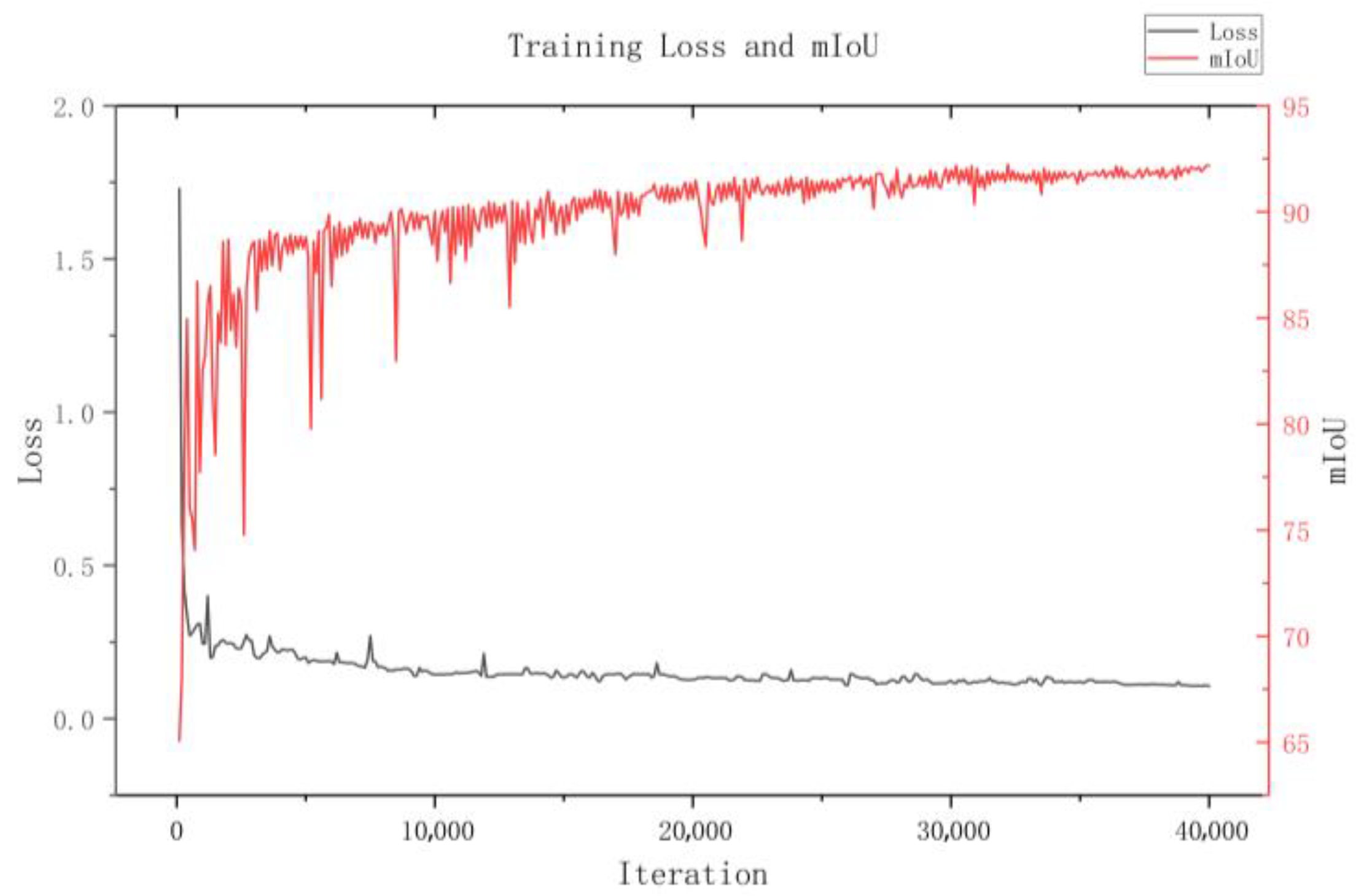
3.2.3. Analysis of the Best Performed Network, K-Net

According to the comparison of the performances of the different neural networks, K-Net performed best in terms of the main evaluation metric, mIoU.

As shown in Figure 11, the training curves of loss and mIoU are presented.

The Loss value drops sharply to 0.2 within the first 10,000 iterations. In the early stages of training, the network quickly learns the prominent features of the data and begins to effectively reduce prediction error. From the 10,000th to the 40,000th iteration, the Loss value decreases gently to 0.1. Although the curve fluctuates, these fluctuations gradually decrease, indicating that, as training progresses, the network continues to learn the subtle features of the data and gradually converges.

The mIoU increases significantly to 91% within the first 20,000 iterations, indicating that the network’s performance in the semantic segmentation task has improved significantly and it can quickly and accurately identify the target areas. During the subsequent 20,000th to 30,000th iterations, it rises slowly to 92%. From the 30,000th to 40,000th iteration, it remains around 92%, and the fluctuations tend to be gentle. This shows that, although the network has already achieved relatively high performance, it continues to learn and fine-tune its predictions to further improve its accuracy.

Although there are mutation points in the Loss and mIoU curves during the training process, the frequency of these mutation points gradually decreases, and the mutation values become progressively smaller. Overall, these mutation points do not significantly impact the network’s overall performance, and the entire training process still shows a good fitting trend.

The confusion matrix reflects the situation of mispredictions among various classes. As shown in

Table 4. The confusion matrix of K-Net.

Class	Duct	AHX	LXF	OVRF	VRFS	EXF	Ground
Duct	0.998
AHX		0.999					0.001
LXF			0.999				0.001
OVRF				1
VRFS					0.999		0.001
EXF						1
ground	0.002	0.001	0.001		0.001		0.997

, except for the background, there is almost no mutual misprediction among components of different classes. However, mispredictions between Duct, AHX, LXF, VRFS, and the background do occur. The reasons for these incorrect predictions are that the edges of semantic segmentation are not perfectly aligned with the actual contours and the perimeters of the components are relatively large. Nevertheless, the nearest neighbor value algorithm has been added in this experiment to match the MEP dictionary, so the impact of these errors on the experimental results can be neglected.

3.3. Generated BIM Results

Dynamo was utilized to read the coordinates and dimensions recorded in Excel to generate a Revit model. The generation sequence is as follows: ducts, equipment, and fittings, as shown in Figure 12, Figure 13 and Figure 14.

Table 5. The process of generating some certain equipment.

Class	Mask and Information Extraction			MEP Component Dictionary		Matched Type	Reconstruction
	Certain Mask	Pixels Count	Area (mm2)	Type List	Defined Area (mm2)
VRF		118,152	738,450	VRF45S VRF56S VRF63S VRF71S	523,480 523,480 670,480 740,480	VRF71S
AHX		257,645	1,610,281	AHX1680 AHX2100	1,628,400 2,215,525	AHX1680
LXF		80,344	502,150	EF-01 EF-02	602,132 502,232	EF-01
OVRF		114,793	717,456	OVRF-01	717,565	OVRF-01
		152,836	955,225	OVRF-02	955,831	OVRF-02
EXF		6375	39,844	EXF-01 EXF-02 EXF-03	40,068 91,192 135,505	EXF-01

lists the processes of some device components, from semantic segmentation and information extraction to type matching to 3D generation.

4. Discussion

4.1. Cases of Prediction Errors in Semantic Segmentation

4.1.1. Incorrect Classification

Since the predicted images are cropped, some only contain a small part of a specific equipment class, with minimal distinction from others, causing incorrect predictions. While the features are still present, they occupy a small portion of the image. The solution is data augmentation, applying operations like rotation, mirroring, and scaling to the images. This helps the neural network learn subtle differences, improving classification accuracy.

4.1.2. Missed Recognition

During the early training with an immature dataset and image predictions, some small sections of ducts and fittings were not detected. This could be due to the ducts being represented by only two parallel thin lines, which made their features less distinguishable. Therefore, during the dataset optimization process, the number of images and annotations for ducts and fittings was significantly increased, with a particular focus on complex and rare scenarios, such as duct fittings and equipment-duct fittings.

4.2. Factors Affecting Coordinate Extraction Accuracy

4.2.1. Pixel Errors in Mask Boundaries

By examining the predicted mask images, it was found that a small portion of the semantic segmentation mask boundaries did not align perfectly with the component contours in the drawing. When zoomed in to the pixel level, the error is typically between 1–2 pixels. This leads to an overall shift in the component coordinates during the bounding box detection. The masks obtained through semantic segmentation are inevitably subject to pixel errors; it is more practical to focus on minimizing the impact of pixel errors during the post-processing stage.

4.2.2. Image Scale

In this experiment, the scale of the image to the actual project is 1 pixel = 2.5 mm, which means the maximum coordinate extraction error is 5 mm for 2 pixels. Therefore, when applying this method to other building MEP projects, the pixel scale of the image is crucial.

The overall slight coordinate shift of the MEP system will not significantly impact O&M. However, if relative errors occur between components, they could affect the connectivity of the MEP model. Therefore, collision and connectivity detection should be performed on the generated model, and any errors should be corrected.

5. Conclusions

This research focuses on the challenges faced by aging buildings during the digital transformation. By integrating semantic segmentation, image processing techniques, and OCR, and Dynamo for automatic generation, a comprehensive solution is developed. This solution aims to efficiently identify and process various equipment and duct components in MEP drawing images, accurately detect their coordinates, and classify them. Furthermore, by counting the number of pixels in the masks obtained from semantic segmentation, or by recognizing their annotations through OCR and matching them with the MEP components dictionary, precise matching of MEP components is achieved. This series of steps enables the automatic generation of BIM from MEP 2D images.

• The MMSegmentation was utilized to call different neural networks to train on the same dataset and conduct a fair performance comparison. Among them, K-Net achieved results with an mIoU of 92.18% and an aAcc of 98.46% during training, verifying the feasibility of using semantic segmentation for MEP drawing recognition. Among other networks, even the lightweight networks have an mIoU exceeding 80%, which validates the rationality of the dataset.
• Gaussian–Laplacian contour detection and minimum bounding box detection are utilized to accurately obtain the coordinates of the components. This process achieved lightweight coordinate detection by simplifying non-essential information in the image. It effectively reduced interfering factors, significantly enhancing the accuracy and reliability of coordinate detection.
• The dimensions of the equipment components are obtained by counting the number of pixels in the bounding box and converting them proportionally. The dimensions of the duct components are obtained through OCR recognition of annotations, which are then associated with the corresponding components.
• The concept of a component dictionary is introduced in this research, which matches extracted component dimensions with preset values in the dictionary and generates the specified model in Revit based on the predefined model type. This method is particularly suitable for MEP components, where the design follows strict standardization and modularization.

Future work will focus on four aspects to broaden the practicality of the proposed method in practical applications:

• Expanding the classes in the dataset and model types in the component dictionary.
• Enhancing the neural network’s ability to recognize components against complex backgrounds in drawings.
• Optimizing the program to automatically detect collisions or disconnections between components and make adjustments accordingly.
• The generated BIM provides data support for VR (Virtual Reality) and AR (Augmented Reality) applications, advancing research on VR and AR-based inspection.

References

1. Nachtigall, F.; Milojevic-Dupont, N.; Wagner, F.C. Predicting building age from urban form at large scale. Comput. Environ. Urban Syst. 2023, 105, 102010. [Google Scholar] [CrossRef]
2. Ramirez, J.P.D.; Nagarsheth, S.H.; Ramirez, C.E.D.; Henao, N.; Agbossou, K. Synthetic dataset generation of energy consumption for residential apartment building in cold weather considering the building’s aging. Data Brief. 2024, 54, 110445. [Google Scholar] [CrossRef] [PubMed]
3. Lee, D.; Cheng, C.C.R. Energy savings by energy management systems: A review. Renew. Sustain. Energy Rev. 2016, 56, 760–777. [Google Scholar] [CrossRef]
4. De Wilde, P. Ten questions concerning building performance analysis. Build. Environ. 2019, 153, 110–117. [Google Scholar] [CrossRef]
5. Utkucu, D.; Szer, H. Interoperability and data exchange within BIM platform to evaluate building energy performance and indoor comfort. Autom. Constr. 2020, 116, 103225. [Google Scholar] [CrossRef]
6. Xiang, Y.; Mahamadu, A.-M.; Florez-Perez, L. Engineering information format utilisation across building design stages: An exploration of BIM applicability in China. J. Build. Eng. 2024, 95, 110030. [Google Scholar] [CrossRef]
7. Kang, T.W.; Choi, H.S. BIM perspective definition metadata for interworking facility management data. Adv. Eng. Inform. 2015, 29, 958–970. [Google Scholar] [CrossRef]
8. Uggla, G.; Horemuz, M. Towards synthesized training data for semantic segmentation of mobile laser scanning point clouds: Generating level crossings from real and synthetic point cloud samples. Autom. Constr. 2021, 130, 103839. [Google Scholar] [CrossRef]
9. Dimitrov, A.; Golparvar-Fard, M. Segmentation of building point cloud models including detailed architectural/structural features and MEP systems. Autom. Constr. 2015, 51, 32–45. [Google Scholar] [CrossRef]
10. Wang, B.; Chen, Z.; Li, M.; Wang, Q.; Yin, C.; Cheng, J.C.P. Omni-Scan2BIM: A ready-to-use Scan2BIM approach based on vision foundation models for MEP scenes. Autom. Constr. 2024, 162, 105384. [Google Scholar] [CrossRef]
11. Wang, J.; Wang, X.; Shou, W.; Chong, H.-Y.; Guo, J. Building information modeling-based integration of MEP layout designs and constructability. Autom. Constr. 2016, 61, 134–146. [Google Scholar] [CrossRef]
12. Park, S.; Shin, M.; Jang, J.Y.; Koo, B.; Kim, T.W. Automated process for generating an air conditioning duct model using the CAD-to-BIM approach. J. Build. Eng. 2024, 91, 109529. [Google Scholar] [CrossRef]
13. Cho, C.Y.; Liu, X.S. An Automated Reconstruction Approach of Mechanical Systems in Building Information Modeling (BIM) Using 2D Drawings. In Proceedings of the IWCCE, Seattle, WA, USA, 25–27 June 2017; pp. 236–244. [Google Scholar]
14. Zou, Q.; Wu, Y.; Liu, Z.; Xu, W.; Gao, S. Intelligent CAD 2.0. Vis. Inform. 2024, 8, 1–12. [Google Scholar] [CrossRef]
15. Jiang, T.; Guo, J.; Xing, W.; Yu, M.; Li, Y.; Zhang, B.; Dong, Y.; Ta, D. A prior segmentation knowledge enhanced deep learning system for the classification of tumors in ultrasound image. Eng. Appl. Artif. Intell. 2025, 142, 109926. [Google Scholar] [CrossRef]
16. Safdar, M.; Li, Y.F.; El Haddad, R.; Zimmermann, M.; Wood, G.; Lamouche, G.; Wanjara, P.; Zhao, Y.F. Accelerated semantic segmentation of additively manufactured metal matrix composites: Generating datasets, evaluating convolutional and transformer models, and developing the MicroSegQ+ Tool. Expert Syst. Appl. 2024, 251, 123974. [Google Scholar] [CrossRef]
17. Zhang, P.; Zhang, S.; Wang, J.; Sun, X. Identifying rice lodging based on semantic segmentation architecture optimization with UAV remote sensing imaging. Comput. Electron. Agric. 2024, 227, 109570. [Google Scholar] [CrossRef]
18. Zhao, Y.; Deng, X.; Lai, H. Reconstructing BIM from 2D structural drawings for existing buildings. Autom. Constr. 2021, 128, 103750. [Google Scholar] [CrossRef]
19. Pan, Z.; Yu, Y.; Xiao, F.; Zhang, J. Recovering building information model from 2D drawings for mechanical, electrical and plumbing systems of ageing buildings. Autom. Constr. 2023, 152, 104914. [Google Scholar] [CrossRef]
20. Zhang, D.; Pu, H.; Li, F.; Ding, X.; Sheng, V.S. Few-Shot Object Detection Based on the Transformer and High-Resolution Network. CMC-Comput. Mater. Contin. 2022, 74, 3439–3454. [Google Scholar] [CrossRef]
21. Wang, C.; Wang, C.; Li, W.; Wang, H. A brief survey on RGB-D semantic segmentation using deep learning. Displays 2021, 70, 102080. [Google Scholar] [CrossRef]
22. Zhao, Z.; Hicks, Y.; Sun, X.; Luo, C. Peach ripeness classification based on a new one-stage instance segmentation model. Comput. Electron. Agric. 2023, 214, 108369. [Google Scholar] [CrossRef]
23. Futakami, N.; Nemoto, T.; Kunieda, E.; Matsumoto, Y.; Sugawara, A. PO-1688 Automatic Detection of Circular Contour Errors Using Convolutional Neural Networks. Radiother. Oncol. 2021, 161, 1414–1415. [Google Scholar] [CrossRef]
24. Gimenez, L.; Robert, S.; Suard, F.; Zreik, K. Automatic reconstruction of 3D building models from scanned 2D floor plans. Autom. Constr. 2016, 63, 48–56. [Google Scholar] [CrossRef]
25. Lu, Q.; Chen, L.; Li, S.; Pitt, M. Semi-automatic geometric digital twinning for existing buildings based on images and CAD drawings. Autom. Constr. 2020, 115, 103183. [Google Scholar] [CrossRef]
26. Sultana, F.; Sufian, A.; Dutta, P. Evolution of Image Segmentation using Deep Convolutional Neural Network: A Survey. Knowl.-Based Syst. 2020, 201–202, 106062. [Google Scholar] [CrossRef]
27. Wang, Y.; Xiao, B.; Bouferguene, A.; Al-Hussein, M.; Li, H. Vision-based method for semantic information extraction in construction by integrating deep learning object detection and image captioning. Adv. Eng. Inform. 2022, 53, 101699. [Google Scholar] [CrossRef]
28. Zhao, Y.; Li, W.; Ding, J.; Wang, Y.; Pei, L.; Tian, A. Crack instance segmentation using splittable transformer and position coordinates. Autom. Constr. 2024, 168, 105838. [Google Scholar] [CrossRef]
29. Chen, J.; Zhuo, L.; Wei, Z.; Zhang, H.; Fu, H.; Jiang, Y.-G. Knowledge driven weights estimation for large-scale few-shot image recognition. Pattern Recogn. 2023, 142, 109668. [Google Scholar] [CrossRef]
30. Kabolizadeh, M.; Rangzan, K.; Habashi, K. Improving classification accuracy for separation of area under crops based on feature selection from multi-temporal images and machine learning algorithms. Adv. Space Res. 2023, 72, 4809–4824. [Google Scholar] [CrossRef]
31. Aimin, Y.; Shanshan, L.; Honglei, L.; Donghao, J. Edge extraction of mineralogical phase based on fractal theory. Chaos Solitons Fractals 2018, 117, 215–221. [Google Scholar] [CrossRef]
32. Mu, K.; Hui, F.; Zhao, X.; Prehofer, C. Multiscale edge fusion for vehicle detection based on difference of Gaussian. Optik 2016, 127, 4794–4798. [Google Scholar] [CrossRef]
33. Tao, X.; Gao, H.; Yang, K.; Wu, Q. Expanding the defect image dataset of composite material coating with enhanced image-to-image translation. Eng. Appl. Artif. Intell. 2024, 133, 108590. [Google Scholar] [CrossRef]
Figure 1. Proposed phases.
Buildings 15 00924 g001
Figure 2. Example of sliding window clipping operation.
Buildings 15 00924 g002
Figure 3. Cropped images.
Buildings 15 00924 g003
Figure 4. Example of sliding window stitching process.
Buildings 15 00924 g004
Figure 5. The overall mask of a certain floor.
Buildings 15 00924 g005
Figure 6. The overall contour image of a certain floor.
Buildings 15 00924 g006
Figure 7. The process of generating the minimum bounding box.
Buildings 15 00924 g007
Figure 8. Image cropping for minimum bounding boxes detection.
Buildings 15 00924 g008
Figure 9. The process of coordinate transformation.
Buildings 15 00924 g009
Figure 10. Forms of augment.
Buildings 15 00924 g010
Figure 11. The training loss and mIoU of K-Net.
Buildings 15 00924 g011
Figure 12. Ducts reconstruction.
Buildings 15 00924 g012
Figure 13. Equipment reconstruction.
Buildings 15 00924 g013
Figure 14. Fittings reconstruction.
Buildings 15 00924 g014