Abstract
Pedestrian flow prediction is a quintessential time series forecasting problem with widespread applications in domains such as indoor navigation and emergency response. However, existing prediction models exhibit sensitivity to anomalous data and face significant challenges in adapting to dynamic and evolving environments. To address these challenges, this paper proposes an integrated pedestrian flow prediction framework. The core architecture employs a Long Short-Term Memory (LSTM) network to capture complex temporal dependencies in pedestrian movement patterns. To improve prediction accuracy, we introduce a two-stage error compensation mechanism. A first-order differential (FoD) module continuously adjusts prediction deviations by analyzing real-time error gradients, while a Hidden Markov Model (HMM)-based adaptive controller dynamically optimizes model parameters in response to changing crowd dynamics. This model effectively mitigates data inconsistency and the challenges associated with a high proportion of zero values. It is designed to provide adaptive feedback and adjust predictions in response to real-time variations in pedestrian flow. For the adjusted time node prediction sequence, accuracy improved by 2.45%, while F-crowded made a significant breakthrough, increasing from 0 to 60.29%. For the full prediction sequence, accuracy increased by 1.9%, from 76.14% to 77.87%, and F-crowded increased by 1.7%, from 85.18% to 86.62%. These results highlight the effectiveness of the HMM-FoD-LSTM model in dealing with data variability in dynamic environments.
1. Introduction
1.1. Time Series Forecasting
The frequent movement of human groups within a given space generates substantial traffic data, the application of which plays a pivotal role in the development of smart cities. In particular, pedestrian traffic, which reflects human activities, can be characterized as a time series within a specific spatial context. A time series comprises a sequence of observations of the same phenomenon over time, exhibiting three key characteristics: trend, serial correlation, and stochasticity [1,2]. Forecasting is a fundamental function of time series analysis, offering significant economic, cultural, and social benefits. Key application areas include finance [3], healthcare [4], environment [5], and transportation [6], among others. Pedestrian Flow Prediction (PFP) is fundamentally a time series forecasting problem, involving the prediction of future pedestrian flows based on a series of observed flow data within a given network [7,8]. PFP can avoid congestion and reduce problems such as falls and slow traffic caused by congestion [9]. It serves as a cornerstone for research in fields such as traffic management, public safety, and route navigation.
The problem of people flow prediction in large public buildings is still not adequately addressed. Existing prediction models are often highly sensitive to anomalous data and cannot fully adapt to the complexity of specific application scenarios. In particular, the performance of the model deteriorates when the proportion of zero data points is high or when data changes exhibit discontinuities. There is also a lack of effective methods to cope with environmental changes. Numerous models have been evaluated for time series forecasting, including AR models [10], Xgboost models (Extreme Gradient Boost model) [11], Long Short-Term Memory (LSTM) networks [12,13,14,15,16,17], and Prophet models [18,19,20], among others. However, these approaches exhibit key limitations in indoor pedestrian flow prediction. AR models [10] assume stationarity and struggle with outliers and sudden changes, limiting their applicability in dynamic indoor settings. Xgboost models [11] perform well with structured data but rely heavily on feature engineering and lack inherent temporal modeling capabilities, reducing their effectiveness for sequential forecasting. LSTM networks [12,13,14,15,16] capture long-term dependencies but are sensitive to zero values, struggle with intermittent patterns, and have fixed gating parameters that hinder real-time adaptation. Prophet models [18,19,20] effectively model seasonality and trends but perform poorly with irregular data and abrupt shifts, which are common in indoor pedestrian flow. Despite advancements in time-series forecasting, existing methods remain inadequate for indoor pedestrian traffic due to the inherent irregularity and non-stationarity of movement patterns. These challenges underscore the need for more adaptive and robust predictive models tailored to dynamic indoor environments.
Among these approaches, deep learning models based on Long Short-Term Memory (LSTM) networks have demonstrated significant potential in predicting pedestrian flow within buildings [21]. Numerous scholars have utilized LSTM as a foundation for pedestrian flow prediction and have made substantial advancements in refining and improving its performance. Du et al. [22] proposed the DST-ICRL LSTM network model for urban traffic flow prediction. Fernandes et al. [23] assessed the accuracy of LSTM models for traffic flow forecasting in data-scarce and non-ideal environments, with their findings highlighting the considerable potential of LSTM networks. Ma et al. [24] mitigated the impact of large eigenvalue ranges by enhancing the traditional LSTM model, subsequently training a bidirectional LSTM network to effectively reduce prediction errors caused by these large eigenvalue variations. Karimzadeh et al. [25] integrated reinforcement learning (RL) and transfer learning (TL) to develop high-performance LSTM predictors. However, the LSTM model still exhibits significant errors in practical applications when environmental conditions change, and it fails to account for anomalous data or address external uncertainties. As such, there is a need for the development of new frameworks that can ensure more stable and accurate pedestrian flow predictions.
1.2. Problem Analysis and Research Questions
Current LSTM-based models for pedestrian flow prediction in large public buildings exhibit several critical limitations:
- Sensitivity to Zero Values and Discontinuities: Model performance deteriorates when the dataset contains a high proportion of zero values or when pedestrian flow patterns exhibit abrupt discontinuities, leading to instability in predictions.
- Limited Adaptability to Irregular Patterns: When pedestrian flow follows atypical periodic patterns, such as those observed during special events, unconventional holidays, or weekends, prediction accuracy remains low. The models lack the capability to dynamically adjust to real-time variations.
- Inadequate Handling of Environmental Changes: Existing methods struggle to effectively incorporate environmental dynamics, often resulting in substantial prediction errors [26].
The current LSTM model is insufficient for addressing the complex and dynamic scenarios involved in indoor pedestrian flow prediction. Consequently, the primary research objective of this paper is to propose a novel LSTM-based model capable of accommodating irregular data inputs and external environmental changes encountered in pedestrian flow prediction. In developing this new model, we address the following key questions:
- Is it possible to propose a novel method that enables the model to perform effectively in the presence of data discontinuity and an excessive proportion of zero values?
- Can an adaptive model tuning approach be developed to address the issue of environmental factor changes, which alter sequence characteristics and impact prediction accuracy in indoor pedestrian traffic forecasting?
- Can the two proposed improvements be integrated to enhance the overall accuracy of the model, ensuring its suitability for the specific application of indoor pedestrian flow prediction?
1.3. Article Structure
In Section 2, Section 2.1 provides a concise overview of the primary models used for pedestrian flow prediction. Section 2.2 provides an introduction to the Long Short-Term Memory (LSTM) model and a review of its current application in pedestrian flow prediction. Section 2.3 explores research on adaptation and self-learning within predictive models. Section 3 describes the framework of the HMM-FoD-LSTM model. Section 4 presents an experimental analysis using real-world data to validate the proposed model, and Section 5 concludes the paper by summarizing the key findings and discussing both the contributions and limitations of this work.
2. Related Work
2.1. Models for Pedestrian Flow Prediction (PFP)
Given the rapid population growth and societal development, pedestrian flow has garnered increasing attention. Accurate pedestrian flow prediction can enhance traffic management, optimize urban infrastructure design [26], mitigate crowding issues during evacuation [27], and provide better solutions for route selection [7]. Pedestrian flow prediction has been the subject of extensive research and development, progressing through three main stages. The first stage is characterized by statistical time series methods, such as AR models; the second stage is marked by the use of XGBoost; and the third stage is dominated by deep learning models, notably Long Short-Term Memory (LSTM) networks. Notably, Prophet, an open-source time series forecasting framework introduced by Facebook in 2017, has not yet been clearly categorized, though it offers distinct advantages. Table 1 presents a compilation and overview of relevant literature.

Table 1.
Review of PFP methods from previous studies.
2.2. Pedestrian Flow Prediction (PFP) with LSTM Model
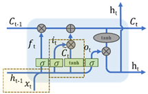
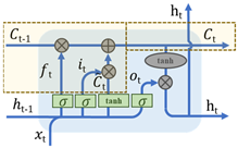
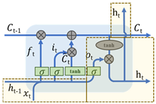
LSTM is a special recurrent neural network (RNN), the specific structure and formula are shown in Table 2 [37]. The input of LSTM includes the cell state , cell hidden layer state and time vector . After a series of operations and adjustments, the cell state and the cell hidden layer state are updated. The gate structure is an important neural network layer of LSTM. It is divided into three types: forgetting gate, input gate, and output gate. The forgetting gate is shown in Formula (1). Using and as input, through , , and sigmoid activation function , an output a vector of 0~1 is used to obtain the information that the cell state needs to be discarded. The first component of the input gate is represented by Formulas (2) and (3), while the second component of the input gate is shown in Formula (4). The output gate is represented by Formulas (5) and (6). LSTM has been widely applied in various fields, including stock analysis [38], industrial output forecasting [39], environmental data forecasting [40], traffic flow research [34], and other domains.
Table 2.
LSTM structure diagram and formula [37,41,42].
A key limitation of current LSTM-based methods for pedestrian flow prediction is the insufficient integration between the prediction model and actual environmental changes. Notable advancements have been made in the field of traffic prediction. For instance, Wang et al. [43] address changes in the driving environment by integrating multiple prediction models to enhance accuracy. These efforts highlight the need for a more adaptive model specifically tailored for pedestrian flow prediction.
As an improved architecture of recurrent neural networks (RNNs), Long Short-Term Memory (LSTM) networks mitigate the gradient vanishing problem of traditional RNN through the gating mechanism and are widely used in the field of time series prediction [37]. However, it still has significant limitations in terms of zero-value sensitivity and dynamic environment adaptation [44], such as zero-value sensitivity with long-term dependency failure, which is essentially due to zero-value interference with the gating mechanism. The forgetting gate and input gate of LSTM rely on the sigmoid function to control the information flow, but when a zero-value persists (e.g., the managed closing time period in the building flow data), the gradient computation may tend to saturate and lead to the failure of the door control unit. For example, in building occupancy prediction, existing models have difficulty distinguishing between managed zeros (e.g., arena closures), leading to over- or under-compensation. Meanwhile, there is also the limitation of long-term memory; although LSTM can deal with long sequence dependency, for intermittent long-period patterns triggered by zeros (e.g., zero nighttime traffic in hospitals), it is difficult for its cellular state to convey effective information across zero-value intervals.
In addition, the lack of adaptability in dynamic environments is another challenge [45], which is due to the conflict between static gating parameters and dynamic changes. The gating weights of LSTM are fixed after training, and it cannot respond to sudden environmental changes in real time. In dynamically changing scenarios, the data distribution may have non-smooth characteristics (e.g., sudden changes in the pattern of holiday crowds). LSTM tends to rely on the local statistical properties of historical data, resulting in insufficient ability to generalize to new patterns. Therefore, Sivakumar [46] combines LSTM with the Hidden Markov Model (HMM) and uses the state transfer property of HMM to dynamically adjust the LSTM gating parameters, which improves the performance of the model.
2.3. Self-Adaptation and Self-Learning in Prediction
Figure 1 presents a generalized schematic diagram of adaptive control. The original model serves as the feedforward input, and upon interacting with the system, the discrepancy between the real data and the model output is measured and fed back into the model. Adaptive control enables the adjustment of the model’s parameters or characteristics, allowing it to continuously adapt to the evolving real-world conditions and external disturbances. Extensive research has been conducted on the adaptive control of systems. Chen et al. [45] proposed the DA-ALQR control algorithm to achieve adaptive control in closed-loop systems. Stepanyan and Lednev [47] investigated target trajectory tracking using an adaptive controller. Ma et al. [48] developed a micro-combustion system optimized through a particle swarm optimization algorithm. Mo [49] introduced a parameter adjustment method to facilitate adaptive control in vehicle dynamic target position tracking.
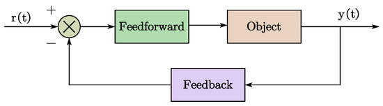
Figure 1.
Schematic diagram of adaptive control.
In the field of sequence prediction, several scholars have explored external adaptation and self-learning techniques, as summarized in Table 3. Generally, external adaptive control systems for prediction sequences exhibit the following characteristics: (a) the integration of multiple algorithms to address external uncertain disturbances, (b) a predominant focus on the dynamic perception of the environment, (c) the application of adaptive control theory to indoor navigation, which has become a key area of research, and (d) a relatively limited number of studies addressing the adaptation of pedestrian flow to external environmental factors.
Table 3.
Adaptive and self-learning related research.
Pedestrian flow prediction plays a crucial role in safety management for smart city development [58], supports indoor staffing and warehouse management [59], and facilitates the safe and efficient operation of mobile robots [60]. Despite these applications, few predictive techniques have been developed to forecast pedestrian flow over time. Furthermore, limited research has addressed the impact of environmental changes on prediction models, which is essential for achieving more accurate results. While some studies have explored the self-adaptation of internal parameters within forecasting models, the adaptation of error adjustments to external environmental changes remains underexplored. Therefore, there is a need for the development of a real-time, adaptive, and accuracy-driven approach [61,62].
3. Methodology
In this paper, we propose an adaptive pedestrian flow prediction model based on first-order differential error adjustment and a Hidden Markov Model, designed to address several key challenges, including the high proportion of zero data, discontinuities, low prediction accuracy at specific nodes, and the inability to dynamically adjust to evolving crowd dynamics. The proposed model is structured in two stages. In the initial stage, the first-order differential (FoD) model continuously corrects prediction deviations by analyzing real-time error gradients. This approach is selected as the optimal solution after comparing five error adjustment methods, as illustrated in the FoD-LSTM module in Figure 2. The second stage integrates a Hidden Markov Model (HMM)-based adaptive controller, which dynamically optimizes model parameters in response to changes in crowd dynamics. The HMM-based controller produces the optimal prediction results by combining threshold adjustment coefficients () after performing probability computations and state partitioning, as shown in the HMM-FoD-LSTM module in Figure 2.
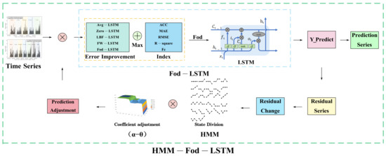
Figure 2.
HMM-Fod-LSTM model flow chart.
3.1. Selection of Error-Adjusted LSTM
Pedestrian flow data is classified as industrial time series, characterized by noise, non-linearity, discontinuities [63], and susceptibility to disturbances. As a result, a single machine learning prediction model often struggles to accurately forecast flow trends. The primary sources of prediction inaccuracies include a high volume of zero data, discontinuous data changes, and prominent outlier feature points. Given these challenges and the observed consistency in forecast trends, it is hypothesized that the errors may be linearly proportional. To address these issues, this paper proposes and evaluates five hybrid models for post-prediction processing. The following five models are considered and tested in this study.
(a) Unmodified scheme (LSTM)
The unmodified LSTM model will serve as a control group, against which the performance and effectiveness of the remaining five models will be compared.
(b) Error adjustment based on mean calculation (Avg-LSTM):
The average of the actual values () is divided by the average of the predicted values () to obtain the linear coefficient, which is then multiplied by the original predicted value. For zero data points, the original predicted value is adjusted by multiplying it with the linear coefficient to obtain the updated predicted value. The deviation, denoted as , is then subtracted from the true value of the zero data points and the new predicted value. Finally, the error-adjusted prediction sequence is calculated based on the average, as shown in Equation (7).
(c) Error adjustment based on zero data weight calculation (Zero-LSTM):
The error-adjusted coefficient is the ratio of the number of training data points in the original sequence to the number of zero data points. The deviation, denoted as , is calculated by subtracting the true value of the zero data points from the newly predicted value. Finally, the weight-adjusted, error-corrected prediction sequence is computed based on zero data, as shown in Equation (8).
(d) Line of best fit based error adjustment (LBF-LSTM):
The best-fit line is obtained by fitting a scatter plot of the actual values () and the predicted values (). The slope of this best-fit line, denoted as , and its reciprocal serve as the linear coefficient for the error adjustment method. The deviation, , is calculated by subtracting the true value of the zero data points from the newly predicted value. Finally, the error-adjusted prediction sequence, , based on the best-fit line, is presented in Equation (9).
(e) Error adjustment based on feature point weight calculation (FW-LSTM):
To mitigate the influence of discrete points, the feature point is selected as the second largest value rather than the maximum value of the actual data (). The linear coefficient for this error adjustment method is determined by multiplying the second largest value of the actual data with the corresponding predicted value (). The deviation, , is calculated by subtracting the actual value of the zero data points from the newly predicted value. Finally, the error adjustment based on the feature point weight is applied, and the resulting prediction sequence, , is presented in Equation (10).
(f) Error adjustment based on first-order difference (Fod-LSTM):
The sequence of predicted values () is determined by ordering the values from largest to smallest and then subtracting each successive value to obtain the first-order difference, (Equation (11)). The linear coefficient for the error adjustment method is calculated as the sum of the sequence numbers divided by . The deviation, , is computed by subtracting the true value of the zero data points from the newly predicted value. Finally, the prediction sequence, , is adjusted based on the first-order difference error, as shown in Equation (12).
3.2. HMM-Based and Error-Adjusted LSTM
Hidden Markov Models (HMMs) are fundamental statistical models in time series forecasting. These models are constructed based on a dynamic Bayesian network, addressing the challenges of probability calculation, prediction, and learning by segmenting states and performing state probability analysis. HMMs have been widely applied in fields such as natural language processing [64,65] and bioinformatics [66]. The number of hidden states in a Hidden Markov Model (denoted as ) is determined by the adjacent sample change states () and the number of consecutive samples (), forming a state transition probability matrix with elements [5]. For example, with two consecutive samples, when the adjacent sample changes among increasing, decreasing, and unchanged, there are three hidden states. With three consecutive samples, there are 9 hidden states, and with four consecutive samples, there are 27 hidden states, as illustrated in Figure 3.
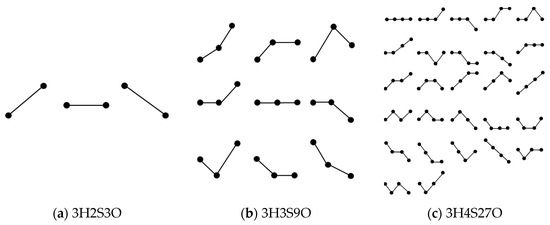
Figure 3.
The changing state of different numbers of adjacent samples in 3 hidden states in HMM.
This paper integrates the state probability estimation concept from the Hidden Markov Model (HMM) into the Error Adjustment-LSTM model, resulting in the HMM-Error Adjustment-LSTM model. This integrated approach enables adaptive error correction in time series forecasting based on environmental changes. The flowchart of the HMM-Error Adjustment-LSTM model is presented in Figure 4.
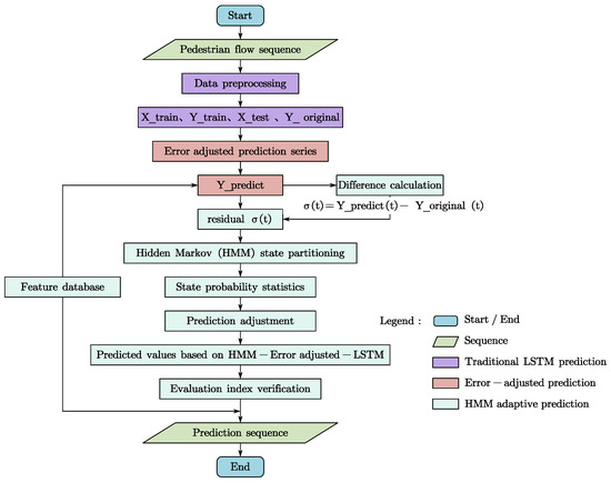
Figure 4.
Flow chart of dynamic adjustment of prediction error based on Hidden Markov Model.
The residual sequence is derived by comparing the predicted values () with the actual data () at the corresponding time node (). This residual sequence is then classified based on the hidden states of the Hidden Markov Model (HMM), with the probability and frequency of each state being computed. The sequence of different hidden states is subsequently adjusted using an adjustment coefficient to obtain the final prediction sequence, which is based on the output of the HMM-Error Adjustment-LSTM model. The model’s prediction accuracy is evaluated using standard performance metrics. If accuracy improves, the corresponding adjustment coefficient and method for determining the hidden state are recorded, and the semantic information associated with the time node is added to the feature database. This semantic information is then fed back into the prediction process to guide model adjustments when predicting similar time nodes in the future. Ultimately, the model outputs a high-accuracy prediction sequence.
3.3. Evaluation Method
Evaluation metrics for time series forecasting typically include accuracy (), error (), absolute error (), percentage error (), mean absolute error (), root mean square error (), mean absolute percentage error (), among others. Guo et al. [67] employed RMSE, MAE, and MAPE to predict highway vehicle flow. Li et al. [68] utilized RMSE and MAE, while Meng et al. [69] selected MAE, MSE, and R-squared for traffic speed prediction. The evaluation metrics commonly used in recent literature are summarized in Table 4.
Table 4.
Evaluation indexes for pedestrian flow prediction.
Unlike other traffic flow time series evaluation metrics, this paper emphasizes accuracy and F-crowded as the primary evaluation indicators. Accuracy is defined as the ratio of nodes where the predicted values match the actual values to the total number of nodes, providing an overall measure of prediction reliability. A higher accuracy index indicates better model performance. F-crowded (denoted as ) refers to the ratio of nodes in the predicted data that exceed the congestion threshold and align with the actual values, relative to the total number of nodes. The closer this index is to 1, the more reliable and realistic the model’s prediction of congestion points is. Consequently, from a goal-oriented perspective, both accuracy and F-crowded are critical for assessing the model’s effectiveness in predicting congestion points, which is particularly relevant to the objective of managing congestion in large public buildings.
4. Experiments and Result Analysis
4.1. Data Collection
This paper utilizes cameras as the primary source of pedestrian flow data. Initially, the cameras capture images of indoor environments within public buildings, from which regions exhibiting pedestrian movement are selected to construct the indoor pedestrian dataset. The Faster-RCNN network is employed to detect pedestrians within these indoor environments, focusing exclusively on individuals to build the dataset. A pre-trained Faster-RCNN model is used for pedestrian identification, while the Mean-Shift and CamShift algorithms are applied to track and count multiple pedestrian targets within the images. The camera model used is the Dahua network hemispherical camera DH-HOBW3236R, as shown in Figure 5, with its monitoring range depicted in Figure 6. Time-series data are collected at 1-min intervals over a period of 28 days (24 h per day, 60 min per hour), resulting in a total of 40,320 consecutive time nodes, each associated with corresponding pedestrian flow data. Manual supervision is applied to enhance the authenticity of the data and eliminate any missing values. The camera is strategically positioned at the back entrance of a large public building, capturing pedestrian movement primarily from employees and customers.
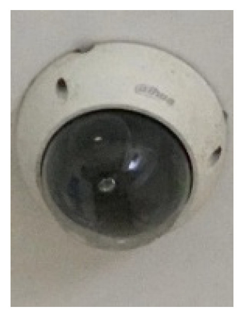
Figure 5.
Surveillance camera.
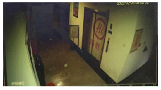
Figure 6.
Surveillance video environment range.
In this scenario, a clear distinction is made between weekdays and weekends. Figure 7a illustrates the pedestrian flow data for weekdays, while Figure 7b presents the pedestrian flow data for weekends.
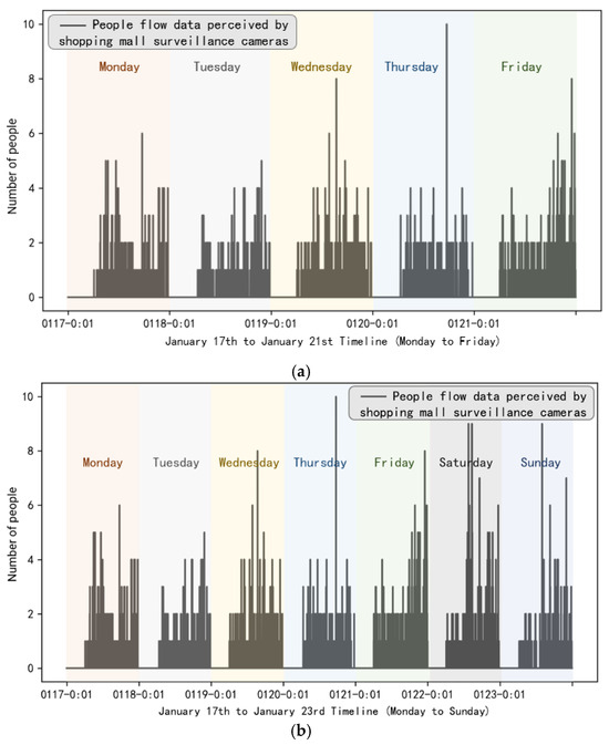
Figure 7.
(a) Example of pedestrian flow data on weekdays (Monday to Friday). (b) Example of pedestrian flow data on weekdays and weekends (Monday to Sunday).
It can be observed that the pedestrian flow patterns on weekends differ from those on weekdays. Notably, there is no peak around 17:30, and pedestrian activity is more pronounced in the afternoon. There is an absence of people during the first 6 h, followed by a peak in traffic after 9:00. As illustrated in Figure 8, the period from 0:00 to 6:00 is characterized by no activity, and afternoon pedestrian flow is significantly higher than in the morning. Moreover, the total number of customers on weekends is substantially greater than on weekdays.
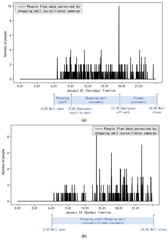
Figure 8.
(a) Analysis of the single-day timeline on weekdays. (b) Analysis of the single-day timeline on weekends.
In conclusion, the data selected for this study exhibit clear periodicity and stability, providing a solid foundation for subsequent pedestrian flow prediction experiments. Furthermore, the distinct patterns observed between weekends and weekdays highlight the influence of real-world environmental changes on prediction outcomes, making this dataset suitable for use in adaptive pedestrian flow prediction models.
The computer hardware configuration used in this experiment consists of an Intel(R) Core (TM) i7-10750H CPU with a base frequency of 2.60 GHz and 64 GB of RAM. Model training and testing were performed using Matlab 2020a and Python 3.6. The parameter settings are outlined in Table 5. The experiment is conducted over four cycles, each lasting five working days, with 1440 data points per cycle, resulting in a total of 7200 complete experimental data points.
Table 5.
Parameter settings.
The comparison of the methods utilized in this study, along with their corresponding data sources, is presented in Figure 9. A total of 7200 data points were employed to assess the prediction performance of the traditional LSTM model and the five error-adjustment models (Section 3.1, Selection of Error-adjusted LSTM), with the goal of selecting the optimal Fod-LSTM model. Additionally, data from 4 weeks of weekdays (20 days, totaling 28,800 data points) were used to compare and evaluate the prediction performance of the Fod-LSTM model against the traditional LSTM model. Furthermore, data from four weeks, including both weekdays and rest weekends (28 days, totaling 40,320 data points), were used to examine the impact of external real-world environmental changes on model prediction performance. This comparison highlights the difference between the error-adjusted LSTM applied to a 7-day cycle and a 5-day cycle. Lastly, a total of 30,240 data points were used to implement the HMM-Fod-LSTM model and assess its prediction accuracy.
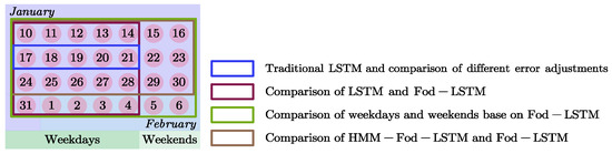
Figure 9.
Correspondence between experimental data and prediction model.
4.2. Traditional LSTM
One set of cycle data is selected for illustration. Figure 10 displays the actual values () for the first four days of training, as well as the actual values () and predicted values () for the final day of testing. Figure 11 presents the discrepancy between the actual values () and the predicted values () on the fifth day. Figure 12 illustrates the relative error between the predicted values () and the actual values () on the same day. Finally, Figure 13 presents a scatter plot comparing the predicted values () with the actual values (), along with the line of best fit and R-squared.
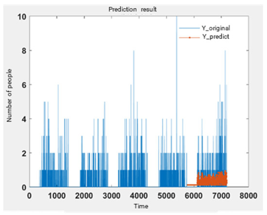
Figure 10.
Five-day Y-train and Y-test prediction results.
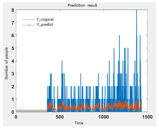
Figure 11.
Single-day Y-train and Y-test prediction results.
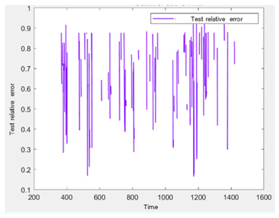
Figure 12.
Relative error of LSTM in a single day.
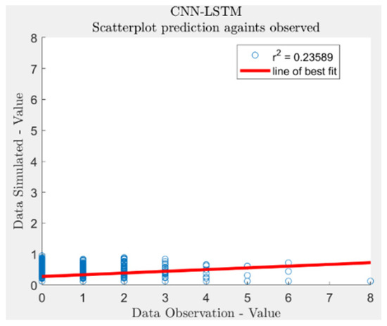
Figure 13.
Scatter plot of the comparison between the actual value and the predicted value in a single day.
It is observed that there is a significant discrepancy between the predicted and actual values; however, the overall trend in pedestrian flow-whether increasing or decreasing-remains consistent. The primary sources of error are the general upward shift in the predicted sequence, the large relative errors at specific nodes, and the considerable deviation of the slope of the best fit line from 1. This discrepancy can be attributed to the high proportion of zero data points within the time series, as well as the discontinuous nature of the data changes.
4.3. Error-Adjusted LSTM
Taking the five working days of the second cycle as an example, the five error adjustment methods are applied to compute the forecast, as illustrated in Figure 14. The blue line represents the actual values (), while the orange line represents the error-adjusted forecast () for the corresponding day. It is evident that, after error adjustment, the forecast trend remains consistent with the original time series. Furthermore, the numerical values show a significant increase compared to the unadjusted model, aligning more closely with the actual observations.
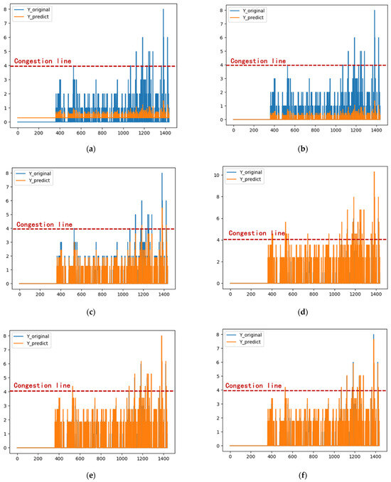
Figure 14.
Error adjustment scheme. (a) Unmodified scheme (LSTM); (b) Error adjustment based on mean calculation (Avg-LSTM); (c) Error adjustment based on zero data weight calculation (Zero-LSTM); (d) Line of best fit based error adjustment (LBF-LSTM); (e) Error adjustment based on feature point weight calculation (FW-LSTM); (f) Error adjustment based on first-order difference (Fod-LSTM).
Table 4 presents the prediction and evaluation indicators, with Table 6 showing the accuracy rates obtained by the unadjusted scheme and the various adjustment schemes. It is evident that, in terms of the accuracy rate (ACC), schemes b and f outperform the unadjusted scheme (a). Regarding the mean absolute error (MAE), the error associated with the error adjustments based on mean calculation (Avg-LSTM) and zero data weight calculation (Zero-LSTM) is smaller than that of the unadjusted LSTM. In terms of root mean square error (RMSE), the unadjusted LSTM performs the best. For the coefficient of determination (R-square), all improved schemes, except scheme d, outperform the unadjusted LSTM, with the coefficient of Error adjustment based on zero data weight calculation (Zero-LSTM) being closest to 1. Concerning crowded point accuracy (Fc), the error adjustment based on first-order difference (Fod-LSTM) significantly outperforms all other improved schemes, achieving 100% accuracy in predicting crowded points.
Table 6.
Index comparison table of data from January 17th to 21st under different improvement schemes.
To comprehensively evaluate the effectiveness of the improved schemes, this paper assigns scores to the five evaluation indicators individually. For the MAE, RMSE, and R-square indicators, the best-performing scheme is awarded 6 points, with scores decreasing progressively to 1 point. For the more critical ACC and Fc indicators, three levels of scoring are applied: 6 points, 3 points, and 1 point. Specifically, for the ACC indicator, the two highest-performing schemes receive 6 points, the next two receive 3 points, and the lowest two receive 1 point. For the Fc indicator, the scheme achieving a score of 1 (i.e., 100%) receives 6 points, those within 1 point of 1 are awarded 3 points, and those exceeding 1 receive 1 point. The indicator scores for the unadjusted and various adjusted schemes are presented in Table 6, with a visualized radar chart shown in Figure 15. It is evident that the Error adjustment based on first-order difference (Fod-LSTM) outperforms the other schemes, excelling in the ACC, Fc, and R-square indicators, and ranking at a medium level for MAE and RMSE.
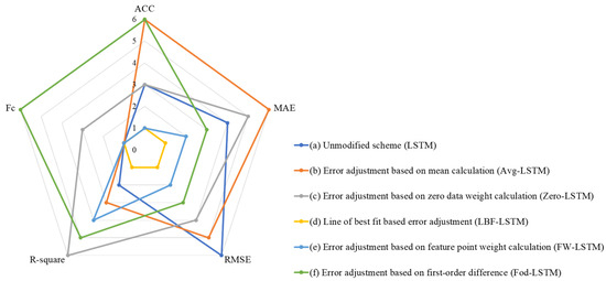
Figure 15.
The data from January 17 to 21 compares the radar chart of indicators under different improvement schemes.
The results demonstrate that the Error Adjustment based on First-Order Difference (Fod-LSTM) outperforms the other models. Fod-LSTM is an LSTM time series forecasting model that incorporates error adjustment based on the first-order difference. In the experiment, Fod-LSTM achieved a 100% accuracy in crowded point prediction and a coefficient of determination of 1.5776. This error adjustment scheme was applied to four additional four-week (20-day) time series periods, and the resulting prediction outcomes, as shown in Figure 16, indicate that Fod-LSTM provides more accurate predictions than the unmodified LSTM model. As summarized in Table 7, the average accuracy (ACC) for the four-week time series data predicted by the unmodified LSTM model is 78.06%, while the average ACC for the Fod-LSTM model is 81.71%, representing a 4.7% improvement over the unmodified model. Additionally, the average crowded point accuracy (Fc) for the LSTM model is 0.00%, whereas the Fod-LSTM model achieves an average Fc of 80.36%, marking a significant improvement from zero to high accuracy, with the Fc for the first and second weeks reaching 100%. Moreover, the Fod-LSTM model shows a noticeable improvement in accuracy and crowded point prediction compared to the unmodified LSTM model, while exhibiting slightly inferior performance in terms of mean absolute error (MAE) and root mean square error (RMSE). However, the coefficient of determination (R-square) remains comparable between the two models.
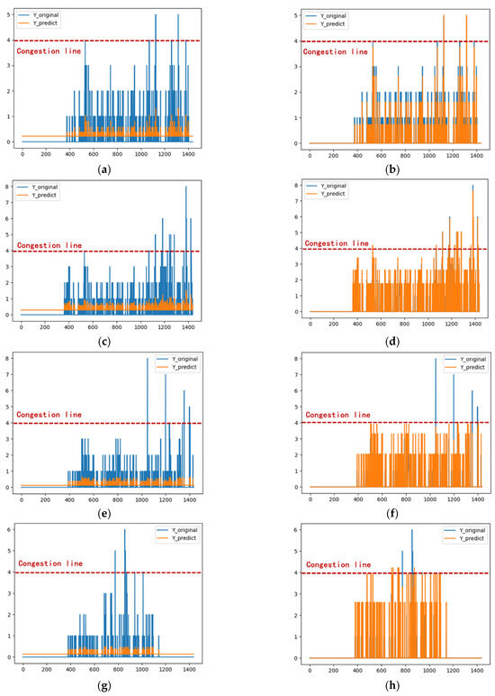
Figure 16.
Comparison of LSTM and Fod-LSTM prediction results (weekdays). (a) LSTM 1.10–1.14; (b) Fod-LSTM 1.10–1.14; (c) LSTM 1.17–1.21; (d) Fod-LSTM 1.17–1.21; (e) LSTM 1.24–1.28; (f) Fod-LSTM 1.24–1.28; (g) LSTM 1.31–2.4; (h) Fod-LSTM 1.31–2.4.
Table 7.
Comparison of evaluation indicators of four-week data under LSTM model and Fod-LSTM model (weekdays).
Thus, for the purpose of pedestrian flow prediction, the Fod-LSTM model effectively estimates crowd density, addressing issues such as data inconsistencies and the prevalence of zero data points.
4.4. HMM-Fod-LSTM
Upon applying the Fod-LSTM model to a 7-day time series (with a train: test ratio of 5:2 as per the parameter settings), the prediction results, shown in Figure 17, can be compared with the evaluation metrics in Table 8. Except for the fourth week, which exhibited higher prediction accuracy, the average accuracy for the remaining three weeks was only 77.25%, with the average deviation of the crowded point accuracy from 100% reaching 46.79%. This indicates that the prediction performance is significantly inferior compared to the 5-day time series. The higher accuracy in the fourth week can be attributed to the public holidays during this period, where the shopping mall’s operating hours were fixed. This suggests that the Fod-LSTM model struggles to adapt to dynamic environmental changes.
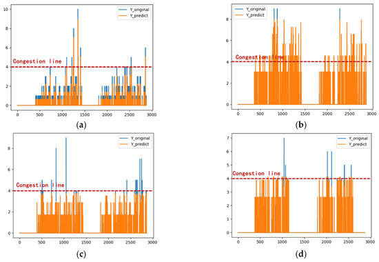
Figure 17.
Time series forecasting diagram based on Fod-LSTM (weekdays plus weekends). (a) 1.10–1.16; (b) 1.17–1.23; (c) 1.24–1.30; (d) 1.31–2.6.
Table 8.
Comparison of evaluation indicators under Fod-LSTM for 28 days of data in four weeks (weekdays plus weekends).
The original flow values of the test data are denoted as . After applying the Fod-LSTM model, the predicted sequence is obtained. Each element of is paired with its corresponding predicted value in based on the time node . The difference between these values is then calculated, as shown in Equation (20), resulting in the residual sequence , which is represented in Equation (21). Based on the hidden state division scheme of the HMM, the corresponding hidden states are then determined.
This experimental case considers a combination of three adjacent sample change states, three consecutive sample numbers, and nine hidden states, forming a state transition probability matrix with 27 elements.
- If the residual change (as shown in Equation (22)) is greater than or equal to the threshold , the time node is assigned to the “increase” state.
- If is less than or equal to the threshold , the time node belongs to the “decrease” state.
- If lies between and , the time node is categorized as the “unchanged” state.
Subsequently, the predicted value is adaptively adjusted, as shown in Equation (23). The adjustment coefficient, , is applied as follows:
- For the “increase” state, is multiplied by ;
- For the “decrease” state, is multiplied by ;
- In other cases, the predicted value remains unchanged.
Various threshold-adjustment coefficient combinations () are generated through exhaustive enumeration, and the optimal () combination is determined. The predicted values are then substituted into the HMM dynamic adjustment model with the optimal () combination to obtain the HMM-Fod-LSTM-based prediction sequence. The prediction results are evaluated and compared using the HMM prediction evaluation indicators. Simultaneously, the adjusted time node and its corresponding semantic information are stored in the database, where they are fed back into the prediction process to facilitate adjustments for similar time nodes with comparable features. The specific algorithm is illustrated in Figure 18.
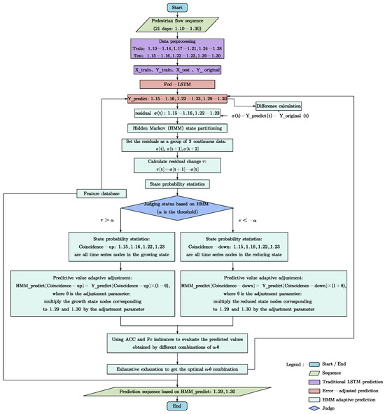
Figure 18.
HMM-Fod-LSTM time series adaptive prediction algorithm.
Through exhaustive evaluations and index assessments of various threshold-adjustment coefficient () combinations, the relationship diagram shown in Figure 19 was obtained. When the threshold and the adjustment coefficient , both the accuracy () and crowded point accuracy () are higher than those of the original predicted sequence.
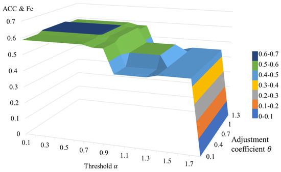
Figure 19.
Changes of important evaluation indicators (ACC and Fc) under different thresholds and adjustment coefficients.
- For thresholds , no time nodes belong to the “increasing” state, while 68 time nodes are classified as the “decreasing” state. When or , both and , evaluated based on the adjusted time nodes (not all predicted nodes), are 58.82%. When , and increase to 60.29%;
- For thresholds , no time nodes belong to the “increasing” state, while 54 time nodes are classified as the “decreasing” state. When or , and are both 57.41%. In contrast, when , and improve to 59.26%;
- For thresholds , no time nodes belong to the “increasing” state, and 14 time nodes are classified as the “decreasing” state. When or , both and are 42.86%. However, when , and increase to 50.00%;
- For thresholds no time nodes belong to the “increasing” state, and nine time nodes are classified as the “decreasing” state. In this case, and are independent of the adjustment coefficient and remain at 44.44%;
- For thresholds , no time nodes belong to the “increasing” state, while only one time node is classified as the “decreasing” state. Here, and are unaffected by , both registering as 0%.
Therefore, when the threshold and the adjustment coefficient , the prediction results are optimized. For the adjusted time node prediction sequence, the improved by 2.45%, while achieved a significant breakthrough, increasing from 0 to 60.29%. For the complete predicted sequence, rose by 1.9%, from 76.14% to 77.87%, and increased by 1.7%, from 85.18% to 86.62%. These results highlight the effectiveness of the HMM-FoD-LSTM model in addressing data variability in dynamic environments.
5. Conclusions
This study proposes an adaptive time series forecasting model based on the LSTM architecture, designed to predict future pedestrian flow data with high accuracy. The model comprises three components: the traditional LSTM, the first-order difference error-adjusted LSTM (Fod-LSTM), and the Hidden Markov adaptive dynamically adjusted LSTM (HMM-Fod-LSTM). This framework addresses critical challenges, including the high proportion of zero-value data, discontinuities, low prediction accuracy for special nodes, and the inability to dynamically adapt predictions to real-world environmental changes.
Experimental simulations using real-world data validate the effectiveness of the proposed HMM-Fod-LSTM model. The results demonstrate that the HMM-Fod-LSTM framework achieves dynamic adaptation in pedestrian flow prediction by integrating the feedforward Fod-LSTM model with a feedback HMM-based adjustment mechanism. When discrepancies arise between predicted and actual data, the HMM identifies hidden states, computes probability statistics, and derives an optimal threshold-adjustment coefficient combination () for specific time nodes, thereby enhancing the prediction accuracy for similar conditions. This study offers a novel approach to improving LSTM-based models and contributes to advancing deep learning techniques in pedestrian flow prediction. The HMM-Fod-LSTM framework demonstrates significant practical utility by enabling dynamic adaptation of pedestrian flow predictions to diverse real-world scenarios. Specifically, it facilitates proactive crowd management through three critical applications: optimization of evacuation routes during indoor emergencies (e.g., fire incidents or security threats), real-time allocation of safety resources in spatially heterogeneous flow regions, and mitigation of congestion risks at transportation hubs through anticipatory capacity planning. Notably, the model’s feedback-driven architecture ensures operational resilience when addressing abrupt density fluctuations caused by irregular events, including transit delays, emergency evacuations, or crowd surges during public gatherings. Such capabilities directly enhance both safety protocols and infrastructure efficiency in high-stakes environments.
In addition, given the similarities between different types of public buildings, we believe our study can be applied to pedestrian flow prediction in large public spaces such as hospitals, airports, and other similar environments. However, to improve prediction accuracy in such contexts, a more comprehensive analysis of the factors affecting the results is required. This includes a closer look at the causes behind zero and peak values, as well as the unique operational dynamics of different public buildings. Moreover, uncertainty conditions in these environments are not limited to peak or off-peak times but also involve irregular events, seasonal fluctuations, and unexpected disruptions, such as maintenance activities, emergencies, or sudden closures. These factors can introduce anomalies and inconsistencies in the data, which our model is designed to address effectively, ensuring robust and reliable predictions across varying conditions.
Despite these advancements, certain limitations remain. The model’s performance has not yet been validated in scenarios involving more complex pedestrian flow patterns, and the experimental simulations were conducted using data with limited temporal granularity. In addition, while the proposed model demonstrates promising predictive accuracy, the statistical significance evaluation of the results may not be sufficiently comprehensive. Future research will aim to address this aspect by incorporating more rigorous statistical testing and significance analysis to further enhance the robustness and interpretability of the experimental findings. These issues warrant further investigation in future research endeavors.
Author Contributions
Conceptualization, Y.X. and Y.D.; methodology, Y.X.; software, H.Z.; validation, H.Z., J.D. and Y.X.; formal analysis, H.Z.; investigation, J.D. and Y.X.; resources, Y.D. and J.-R.L.; data curation, J.D.; writing—original draft preparation, H.Z. and J.D.; writing—review and editing, Y.D. and J.-R.L.; visualization, H.Z.; supervision, Y.X.; project administration, Y.D.; funding acquisition, Y.D. All authors have read and agreed to the published version of the manuscript.
Funding
The authors would like to acknowledge the support of the National Science Foundation of China (52308314), and the support of the Guangdong Basic and Applied Basic Research Foundation (2023A1515030169).
Data Availability Statement
The original contributions presented in the study are included in the article, further inquiries can be directed to the corresponding author.
Conflicts of Interest
The authors declare no conflict of interest.
References
- De Gooijer, J.G.; Hyndman, R.J. 25 years of time series forecasting. Int. J. Forecast. 2006, 22, 443–473. [Google Scholar] [CrossRef]
- Parzen, E. An approach to time series analysis. Ann. Math. Stat. 1961, 32, 951–989. [Google Scholar] [CrossRef]
- Sezer, O.B.; Gudelek, M.U.; Ozbayoglu, A.M. Financial time series forecasting with deep learning: A systematic literature review: 2005–2019. Appl. Soft Comput. 2020, 90, 106181. [Google Scholar] [CrossRef]
- Maleki, M.; Mahmoudi, M.R.; Wraith, D.; Pho, K.-H. Time series modelling to forecast the confirmed and recovered cases of COVID-19. Travel Med. Infect. Dis. 2020, 37, 101742. [Google Scholar] [CrossRef]
- Zhang, X.; Zhao, J.; Cai, B. Prediction Model with Dynamic Adjustment for Single Time Series of PM2.5. Acta Autom. Sin. 2018, 44, 1790–1798. [Google Scholar] [CrossRef]
- Li, L.; Su, X.; Zhang, Y.; Lin, Y.; Li, Z. Trend modeling for traffic time series analysis: An integrated study. IEEE Trans. Intell. Transp. Syst. 2015, 16, 3430–3439. [Google Scholar] [CrossRef]
- Liu, M.; Li, L.; Li, Q.; Bai, Y.; Hu, C. Pedestrian flow prediction in open public places using graph convolutional network. ISPRS Int. J. Geo-Inf. 2021, 10, 455. [Google Scholar] [CrossRef]
- Luca, M.; Barlacchi, G.; Lepri, B.; Pappalardo, L. Deep learning for human mobility a survey on data and models. arXiv 2020, arXiv:2012.02825. [Google Scholar]
- Deng, H.; Tian, M.; Ou, Z.; Deng, Y. A semantic framework for on-site evacuation routing based on awareness of obstacle accessibility. Autom. Constr. 2022, 136, 104154. [Google Scholar] [CrossRef]
- Kitagawa, G.; Gersch, W. A smoothness priors time-varying AR coefficient modeling of nonstationary covariance time series. IEEE Trans. Autom. Control. 1985, 30, 48–56. [Google Scholar] [CrossRef]
- Alim, M.; Ye, G.-H.; Guan, P.; Huang, D.-S.; Zhou, B.-S.; Wu, W. Comparison of ARIMA model and XGBoost model for prediction of human brucellosis in mainland China: A time-series study. BMJ Open 2020, 10, e039676. [Google Scholar] [CrossRef]
- Siami-Namini, S.; Tavakoli, N.; Namin, A.S. A comparison of ARIMA and LSTM in forecasting time series. In Proceedings of the 2018 17th IEEE International Conference on Machine Learning and Applications (ICMLA), Orlando, FL, USA, 17–20 December 2018; IEEE: Piscataway, NJ, USA, 2018; pp. 1394–1401. [Google Scholar]
- Song, X.; Liu, Y.; Xue, L.; Wang, J.; Zhang, J.; Wang, J.; Jiang, L.; Cheng, Z. Time-series well performance prediction based on Long Short-Term Memory (LSTM) neural network model. J. Pet. Sci. Eng. 2020, 186, 106682. [Google Scholar] [CrossRef]
- Siami-Namini, S.; Tavakoli, N.; Namin, A.S. The performance of LSTM and BiLSTM in forecasting time series. In Proceedings of the 2019 IEEE International Conference on Big Data (Big Data), Los Angeles, CA, USA, 9–12 December 2019; IEEE: Piscataway, NJ, USA, 2019; pp. 3285–3292. [Google Scholar]
- Gers, F.A.; Eck, D.; Schmidhuber, J. Applying LSTM to time series predictable through time-window approaches. In Neural Nets WIRN Vietri-01; Springer: London, UK, 2002; pp. 193–200. [Google Scholar]
- Greff, K.; Srivastava, R.K.; Koutník, J.; Steunebrink, B.R.; Schmidhuber, J. LSTM: A search space odyssey. IEEE Trans. Neural Netw. Learn. Syst. 2016, 28, 2222–2232. [Google Scholar] [CrossRef] [PubMed]
- Hochreiter, S.; Schmidhuber, J. Long Short-Term Memory. Neural Comput. 1997, 9, 1735–1780. [Google Scholar] [CrossRef] [PubMed]
- Satrio, C.B.A.; Darmawan, W.; Nadia, B.U.; Hanafiah, N. Time series analysis and forecasting of coronavirus disease in Indonesia using ARIMA model and PROPHET. Procedia Comput. Sci. 2021, 179, 524–532. [Google Scholar] [CrossRef]
- Samal, K.K.R.; Babu, K.S.; Das, S.K.; Acharaya, A. Time series based air pollution forecasting using SARIMA and prophet model. In Proceedings of the 2019 International Conference on Information Technology and Computer Communications, Guangzhou, China, 20–22 December 2019; pp. 80–85. [Google Scholar]
- Taylor, S.J.; Letham, B. Forecasting at scale. Am. Stat. 2018, 72, 37–45. [Google Scholar] [CrossRef]
- Alawad, H.; An, M.; Kaewunruen, S. Utilizing an adaptive neuro-fuzzy inference system (ANFIS) for overcrowding level risk assessment in railway stations. Appl. Sci. 2020, 10, 5156. [Google Scholar] [CrossRef]
- Du, B.; Peng, H.; Wang, S.; Alam Bhuiyan, Z.; Wang, L.; Gong, Q.; Liu, L.; Li, J. Deep irregular convolutional residual LSTM for urban traffic passenger flows prediction. IEEE Trans. Intell. Transp. Syst. 2019, 21, 972–985. [Google Scholar] [CrossRef]
- Fernandes, B.; Silva, F.; Alaiz-Moretón, H.; Novais, P.; Analide, C.; Neves, J. Traffic flow forecasting on data-scarce environments using ARIMA and LSTM networks. In Proceedings of the World Conference on Information Systems and Technologies, Galicia, Spain, 16–19 April 2019; Springer: Cham, Switzerland, 2019; pp. 273–282. [Google Scholar]
- Ma, C.; Dai, G.; Zhou, J. Short-term traffic flow prediction for urban road sections based on time series analysis and LSTM_BILSTM method. IEEE Trans. Intell. Transp. Syst. 2021, 23, 5615–5624. [Google Scholar] [CrossRef]
- Karimzadeh, M.; Aebi, R.; de Souza, A.M.; Zhao, Z.; Braun, T.; Sargento, S.; Villas, L. Reinforcement learning-designed LSTM for trajectory and traffic flow prediction. In Proceedings of the 2021 IEEE Wireless Communications and Networking Conference (WCNC), Nanjing, China, 29 March–1 April 2021; IEEE: Piscataway, NJ, USA, 2021; pp. 1–6. [Google Scholar]
- Manibardo, E.L.; Laña, I.; Del Ser, J. Change detection and adaptation strategies for long-term estimation of pedestrian flows. In Proceedings of the 2021 IEEE International Intelligent Transportation Systems Conference (ITSC), Indianapolis, IN, USA, 19–22 September 2021; IEEE: Piscataway, NJ, USA, 2021; pp. 1867–1874. [Google Scholar]
- Wang, D.-W.; Li, L.-N.; Hu, C.; Li, Q.; Chen, X.; Huang, P.-W. A modified inverse distance weighting method for interpolation in open public places based on Wi-Fi probe data. J. Adv. Transp. 2019, 2019, 1–11. [Google Scholar] [CrossRef]
- Lee, R.S.C.; Hughes, R.L. Prediction of human crowd pressures. Accid. Anal. Prev. 2006, 38, 712–722. [Google Scholar] [CrossRef] [PubMed]
- Yan, D.; Zhou, J.; Zhao, Y.; Wu, B. Short-term subway passenger flow prediction based on ARIMA. In Proceedings of the International Conference on Geo-Spatial Knowledge and Intelligence, Chiang Mai, Thailand, 8–10 December 2017; Springer: Singapore, 2017; pp. 464–479. [Google Scholar]
- Liu, D.; Rong, W.; Zhang, J.; Ge, Y.-E. Exploring the Nonlinear Effects of Built Environment on Bus-Transfer Ridership: Take Shanghai as an Example. Appl. Sci. 2022, 12, 5755. [Google Scholar] [CrossRef]
- Cohen, A.; Dalyot, S. Machine-learning prediction models for pedestrian traffic flow levels: Towards optimizing walking routes for blind pedestrians. Trans. GIS 2020, 24, 1264–1279. [Google Scholar] [CrossRef]
- Abrishami, S.; Kumar, P. Using real-world store data for foot traffic forecasting. In Proceedings of the 2018 IEEE International Conference on Big Data (Big Data), Seattle, WS, USA, 10–13 December 2018; IEEE: Piscataway, NJ, USA, 2018; pp. 1885–1890. [Google Scholar]
- Li, C.; Xu, P. Application on traffic flow prediction of machine learning in intelligent transportation. Neural Comput. Appl. 2021, 33, 613–624. [Google Scholar] [CrossRef]
- Essien, A.E.; Chukwkelu, G.; Giannetti, C. A scalable deep convolutional LSTM neural network for large-scale urban traffic flow prediction using recurrence plots. In Proceedings of the 2019 IEEE AFRICON, Accra, Ghana, 25–27 September 2019; IEEE: Piscataway, NJ, USA, 2019; pp. 1–7. [Google Scholar]
- Zhu, J.; Feng, F.; Shen, B. People counting and pedestrian flow statistics based on convolutional neural network and recurrent neural network. In Proceedings of the 2018 33rd Youth Academic Annual Conference of Chinese Association of Automation (YAC), Nanjing, China, 18–20 May 2018; IEEE: Piscataway, NJ, USA, 2018; pp. 993–998. [Google Scholar]
- Shaoji, W.U.; Yike, H.U. Research on Spatial Hyper-Links in Commercial Complexes Based on Deep Learning: A Case Study of TaiKoo Li Sanlitun and Beijing APM. South Archit. 2022, 1, 61–68. [Google Scholar]
- Al-Selwi, S.M.; Hassan, M.F.; Abdulkadir, S.J.; Muneer, A.; Sumiea, E.H.; Alqushaibi, A.; Ragab, M.G. RNN-LSTM: From applications to modeling techniques and beyond—Systematic review. J. King Saud Univ.—Comput. Inf. Sci. 2024, 36, 102068. [Google Scholar] [CrossRef]
- Badri, A.K.; Heikal, J.; Terah, Y.A.; Nurjaman, D.R. Decision-Making Techniques using LSTM on Antam Mining Shares before and during the COVID-19 Pandemic in Indonesia. APTISI Trans. Manag. (ATM) 2022, 6, 167–180. [Google Scholar] [CrossRef]
- Fan, D.; Sun, H.; Yao, J.; Zhang, K.; Yan, X.; Sun, Z. Well production forecasting based on ARIMA-LSTM model considering manual operations. Energy 2021, 220, 119708. [Google Scholar] [CrossRef]
- Yan, R.; Liao, J.; Yang, J.; Sun, W.; Nong, M.; Li, F. Multi-hour and multi-site air quality index forecasting in Beijing using CNN, LSTM, CNN-LSTM, and spatiotemporal clustering. Expert Syst. Appl. 2021, 169, 114513. [Google Scholar] [CrossRef]
- Yu, Y.; Si, X.; Hu, C.; Zhang, J. A review of recurrent neural networks: LSTM cells and network architectures. Neural Comput. 2019, 31, 1235–1270. [Google Scholar] [CrossRef]
- Staudemeyer, R.C.; Morris, E.R. Understanding LSTM—A tutorial into long short-term memory recurrent neural networks. arXiv 2019, arXiv:1909.09586. [Google Scholar]
- Wang, Y.; Yu, C.; Hou, J.; Chu, S.; Zhang, Y.; Zhu, Y. ARIMA Model and Few-Shot Learning for Vehicle Speed Time Series Analysis and Prediction. Comput. Intell. Neurosci. 2022, 2022, 2526821. [Google Scholar] [CrossRef]
- Zheng, H.; Liu, Y.; Wan, W.; Zhao, J.; Xie, G. Large-scale prediction of stream water quality using an interpretable deep learning approach. J. Environ. Manag. 2023, 331, 117309. [Google Scholar] [CrossRef] [PubMed]
- Chen, S.; Li, Q.; Zhou, T.; Lu, S. Multivariable Adaptive Control Algorithm of Variable Cycle Engine Based on Data Driven. J. Propuls. Technol. 2022, 43, 371–382. [Google Scholar] [CrossRef]
- Sivakumar, G. HMM-LSTM Fusion Model for Economic Forecasting[A/OL]. arXiv 2025, arXiv:2501.02002. [Google Scholar]
- Stepanyan, I.V.; Lednev, M.Y. Prediction of the trajectory of the tracking object based on adaptive controller. IOP Conf. Ser. Mater. Sci. Eng. 2020, 747, 12078. [Google Scholar] [CrossRef]
- Ma, C.; Zhu, X.; Han, Y. Application of Adaptive Generalized Predictive Control Based on PSO in Microturbines. Control Eng. China 2019, 26, 179–184. [Google Scholar]
- Mo, S. Model-Free Adaptive Predictive Control for Tracking the Dynamic Target Position of Vehicle. Mach. Des. Manuf. 2018, 12, 1296–1299. [Google Scholar] [CrossRef]
- Zeng, C.; Hua, C.; Lei, T.; Xiao, X. Short-term traffic flow prediction on campus based on modified PSOBP neural network. J. Phys. Conf. Ser. 2020, 1592, 012071. [Google Scholar] [CrossRef]
- Alahakoon, D.; Nawaratne, R.; Xu, Y.; De Silva, D.; Sivarajah, U.; Gupta, B. Self-building artificial intelligence and machine learning to empower big data analytics in smart cities. Inf. Syst. Front. 2020, 25, 221–240. [Google Scholar] [CrossRef]
- Zhang, T.; Yuan, J.; Chen, Y.-C.; Jia, W. Self-learning soft computing algorithms for prediction machines of estimating crowd density. Appl. Soft Comput. 2021, 105, 107240. [Google Scholar] [CrossRef]
- Zhou, Y.; Ravey, A.; Pera, M.C. A velocity prediction method based on self-learning multi-step Markov chain. In Proceedings of the IECON 2019-45th Annual Conference of the IEEE Industrial Electronics Society, Lisbon, Portugal, 14–17 October 2019; IEEE: Piscataway, NJ, USA, 2019; Volume 1, pp. 2598–2603. [Google Scholar]
- Tran, D.P.; Hoang, V.D. Adaptive learning based on tracking and ReIdentifying objects using convolutional neural network. Neural Process. Lett. 2019, 50, 263–282. [Google Scholar] [CrossRef]
- Goldhammer, M.; Kohler, S.; Doll, K.; Sick, B. Camera based pedestrian path prediction by means of polynomial least-squares approximation and multilayer perceptron neural networks. In Proceedings of the 2015 SAI Intelligent Systems Conference (IntelliSys), London, UK, 10–11 November 2015; IEEE: Piscataway, NJ, USA, 2015; pp. 390–399. [Google Scholar]
- George, S.; Santra, A.K. Traffic prediction using multifaceted techniques: A survey. Wirel. Pers. Commun. 2020, 115, 1047–1106. [Google Scholar] [CrossRef]
- Huynh, M.; Alaghband, G. Aol: Adaptive online learning for human trajectory prediction in dynamic video scenes. arXiv 2020, arXiv:2002.06666. [Google Scholar]
- Harrou, F.; Dairi, A.; Zeroual, A.; Sun, Y. Forecasting of Bicycle and Pedestrian Traffic Using Flexible and Efficient Hybrid Deep Learning Approach. Appl. Sci. 2022, 12, 4482. [Google Scholar] [CrossRef]
- Kabak, Ö.; Ülengin, F.; Aktaş, E.; Önsel, Ş.; Topcu, Y.I. Efficient shift scheduling in the retail sector through two-stage optimization. Eur. J. Oper. Res. 2008, 184, 76–90. [Google Scholar] [CrossRef]
- Vintr, T.; Yan, Z.; Eyisoy, K.; Kubiš, F.; Blaha, J.; Ulrich, J.; Swaminathan, C.S.; Molina, S.; Kucner, T.P.; Magnusson, M.; et al. Natural criteria for comparison of pedestrian flow forecasting models. In Proceedings of the 2020 IEEE/RSJ International Conference on Intelligent Robots and Systems (IROS), Detroit, MI, USA, 1–5 October 2023; IEEE: Piscataway, NJ, USA, 2020; pp. 11197–11204. [Google Scholar]
- Thejaswini, R.S.S.; Rajaraajeswari, S. A real-time traffic congestion-avoidance framework for smarter cities. AIP Conf. Proc. 2018, 2039, 020009. [Google Scholar]
- May, M.; Scheider, S.; Rösler, R.; Schulz, D.; Hecker, D. Pedestrian flow prediction in extensive road networks using biased observational data. In Proceedings of the 16th ACM SIGSPATIAL International Conference on Advances in Geographic Information System, Hamburg, Germany, 13–16 November 2023. [Google Scholar]
- Cryer, J.D.; Chan, K.S. Time Series Analysis: With Applications in R; Springer Science & Business Media: Berlin, Germany, 2008. [Google Scholar]
- Rajan, A.; Salgaonkar, A. Part of speech (PoS) tagging for Konkani language using HMM. In ICT Systems and Sustainability; Springer: Singapore, 2022; pp. 601–609. [Google Scholar]
- Anandika, A.; Mishra, S.P.; Das, M. Review on Usage of Hidden Markov Model in Natural Language Processing. In Intelligent and Cloud Computing; Springer: Singapore, 2021; pp. 415–423. [Google Scholar]
- Sharma, R.; Kumar, S.; Tsunoda, T.; Kumarevel, T.; Sharma, A. Single-stranded and double-stranded DNA-binding protein prediction using HMM profiles. Anal. Biochem. 2021, 612, 113954. [Google Scholar] [CrossRef]
- Guo, J.; Xing, S.; Luan, H.; Jia, Y. Prediction of time series traffic based on improved LSTM algorithm. J. Nanjing Univ. Inf. Sci. Technol. (Nat. Sci. Ed.) 2021, 13, 571–675. [Google Scholar] [CrossRef]
- Li, L.; Zhang, Q.; Zhao, J.; Mie, Y. Short-Term Traffic Flow Prediction Method of Different Periods Based on Improved CNN-LSTM. J. Appl. Sci. 2021, 39, 185–198. [Google Scholar]
- Meng, X.; Fu, H.; Peng, L.; Liu, G.; Yu, Y.; Wang, Z.; Chen, E. D-LSTM: Short-term road traffic speed prediction model based on GPS positioning data. IEEE Trans. Intell. Transp. Syst. 2020, 23, 2021–2030. [Google Scholar] [CrossRef]


Disclaimer/Publisher’s Note: The statements, opinions and data contained in all publications are solely those of the individual author(s) and contributor(s) and not of MDPI and/or the editor(s). MDPI and/or the editor(s) disclaim responsibility for any injury to people or property resulting from any ideas, methods, instructions or products referred to in the content. |
© 2025 by the authors. Licensee MDPI, Basel, Switzerland. This article is an open access article distributed under the terms and conditions of the Creative Commons Attribution (CC BY) license (https://creativecommons.org/licenses/by/4.0/).