
Harnessing the Power of Improved Deep Learning for Precise Building Material Price Predictions


Abstract
1. Introduction
2. Data Sources and Analysis
2.1. Data Source
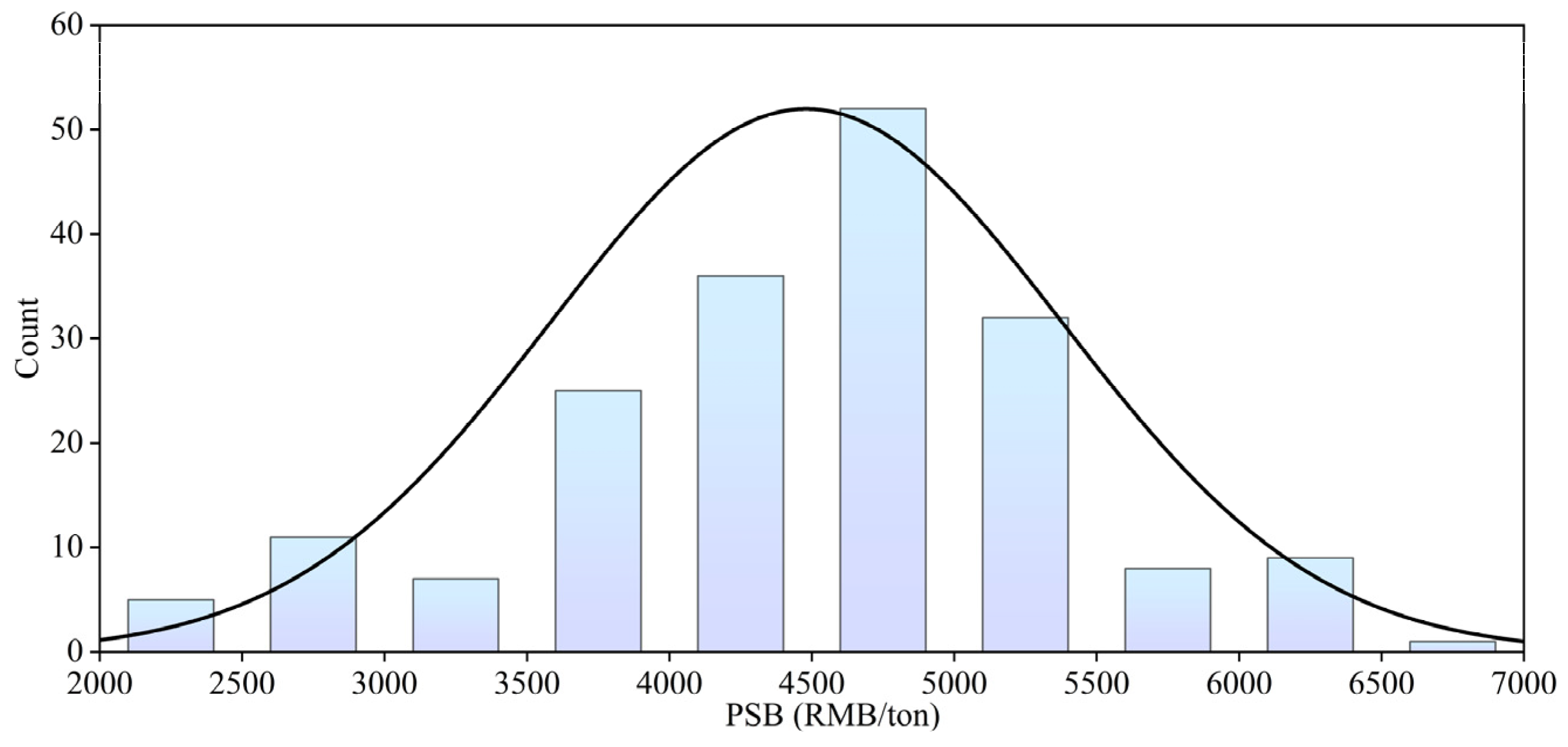
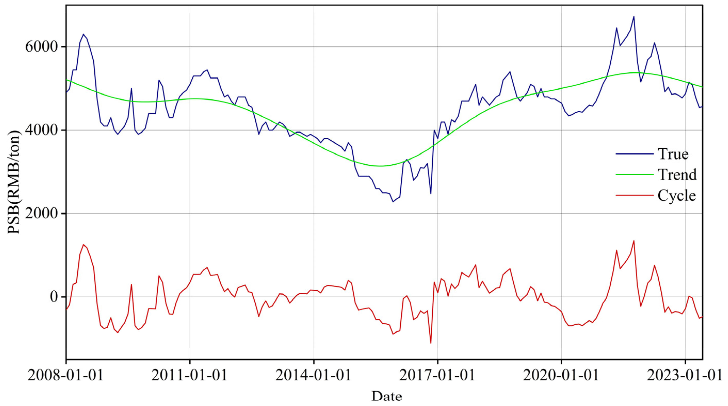
2.2. Data Analysis
3. Methods
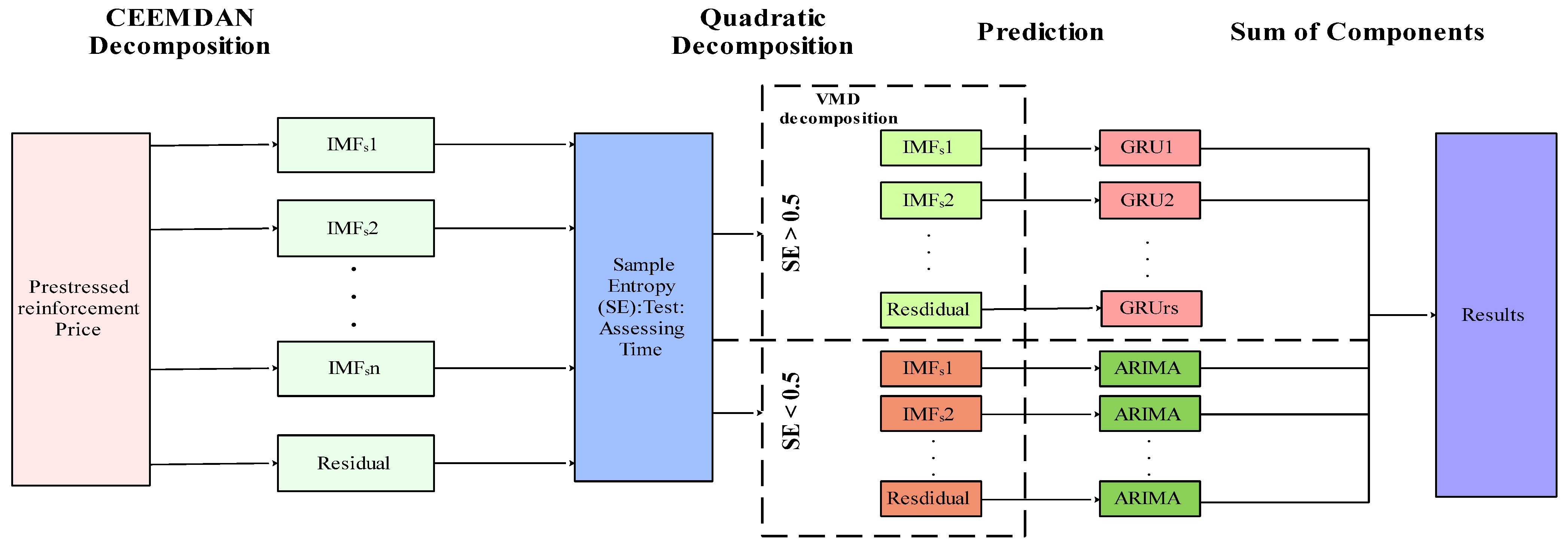
3.1. Integrated Decomposition–Ensemble Model for PSB Market Price Prediction
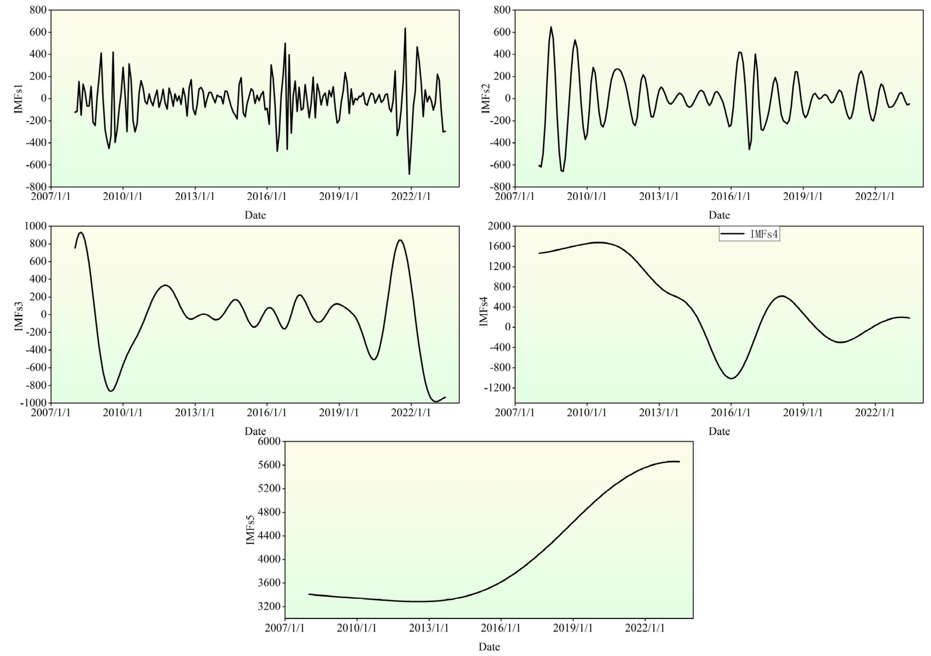
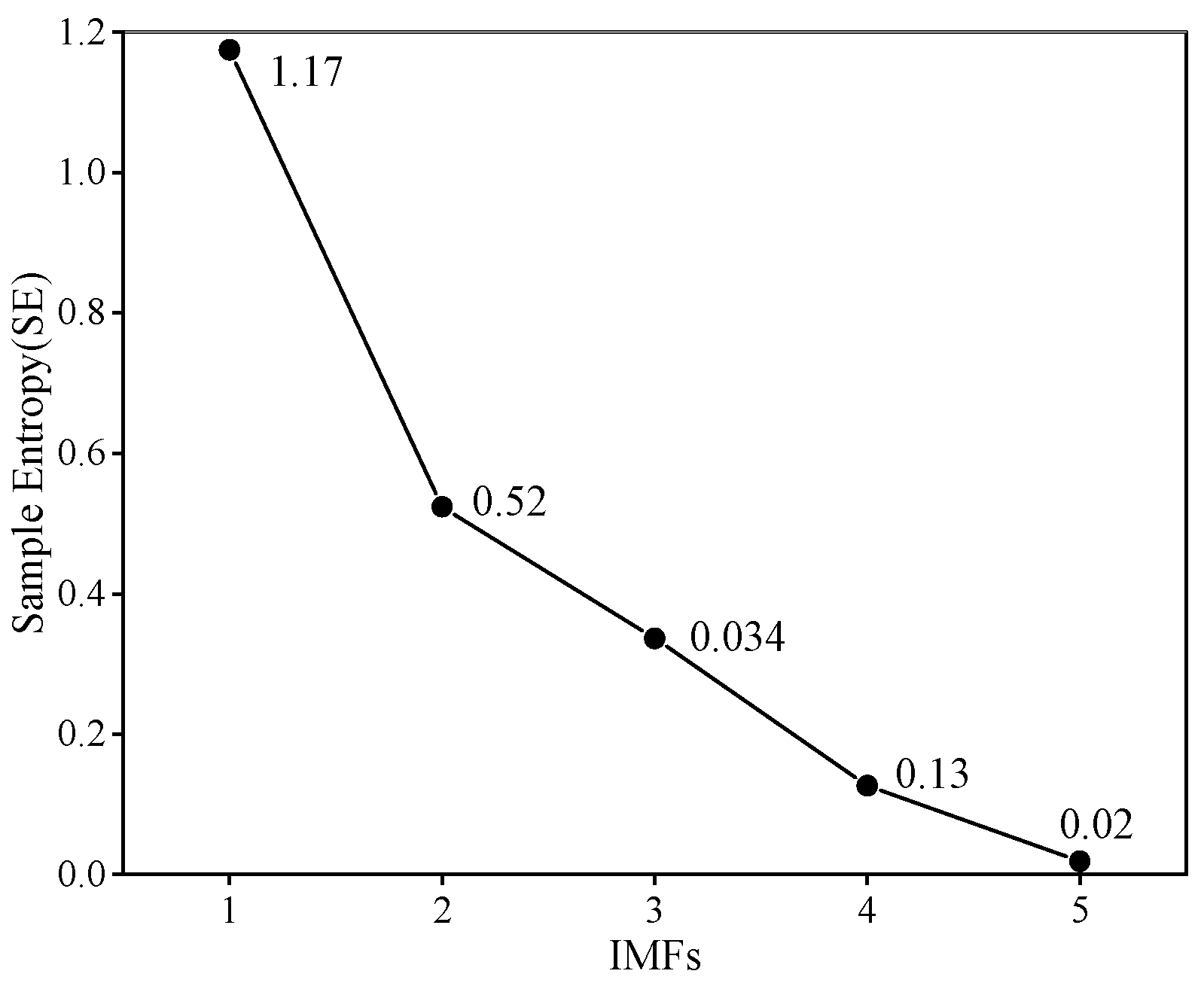
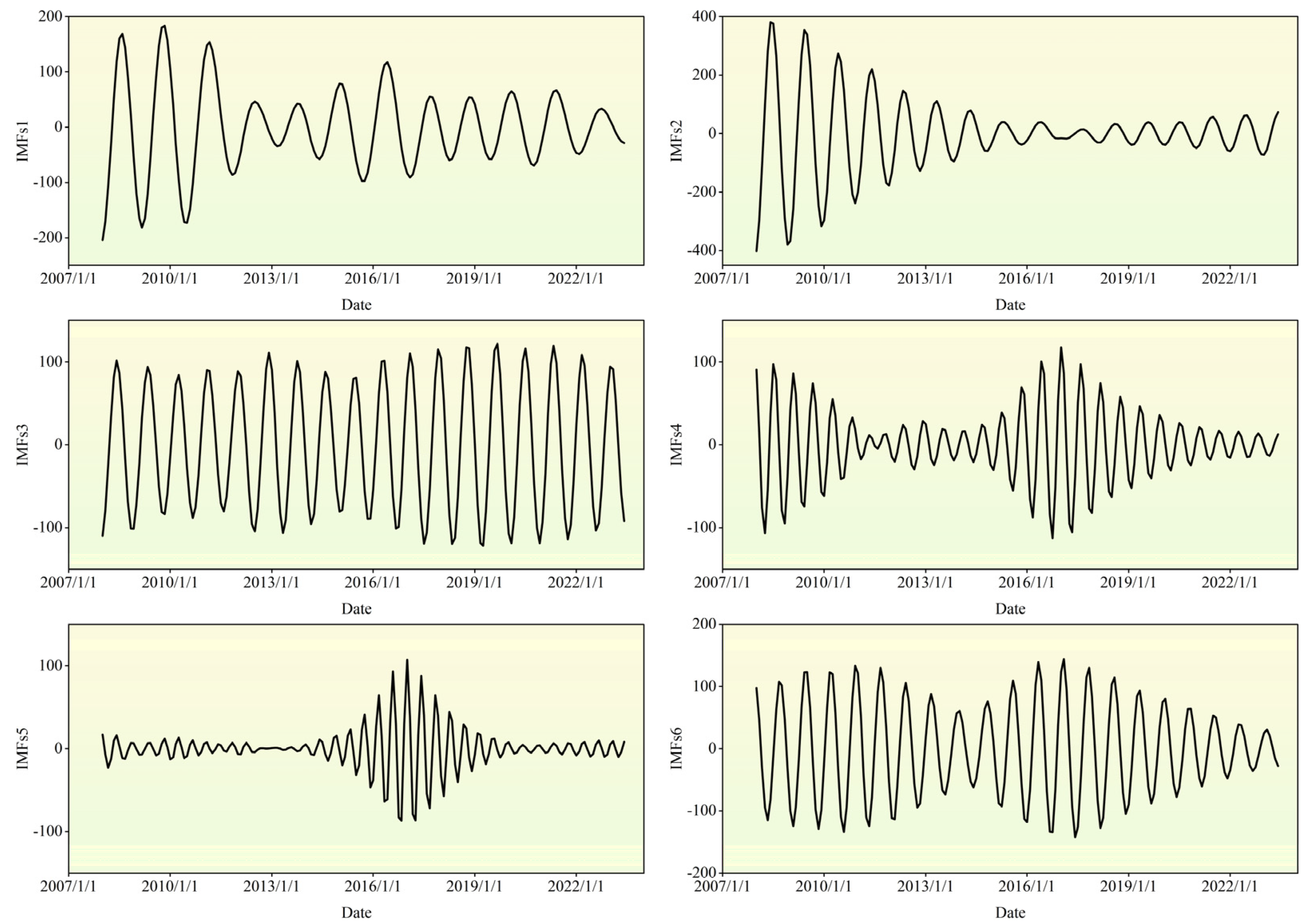
3.1.1. CEEMDAN Model
3.1.2. ARIMA Model
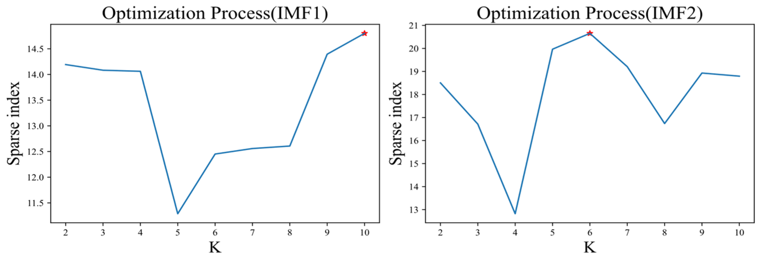
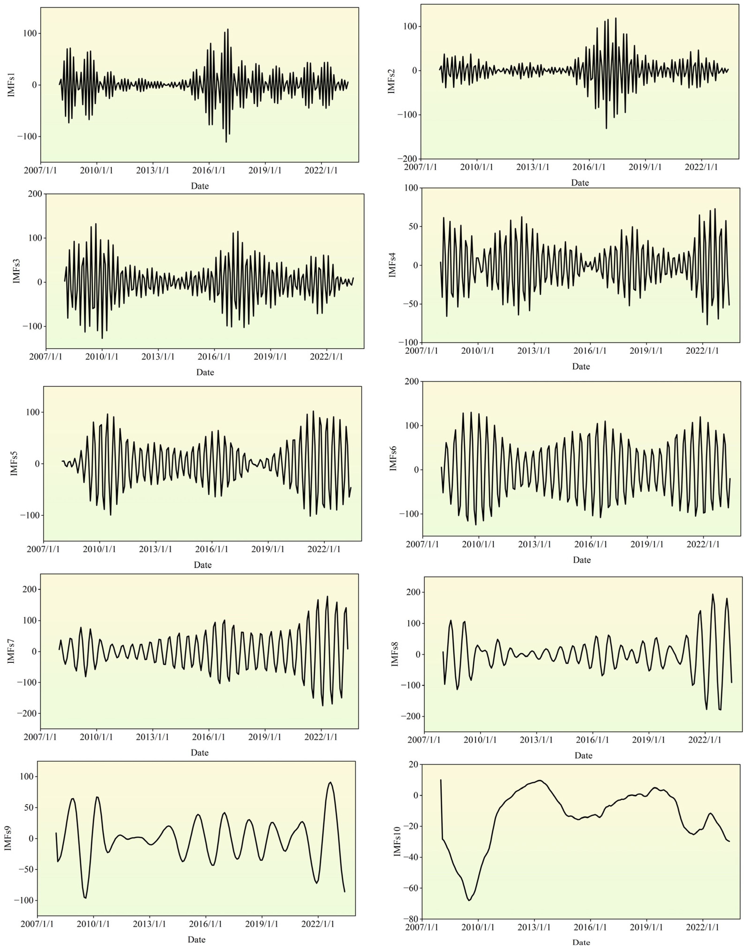
3.1.3. VMD Model
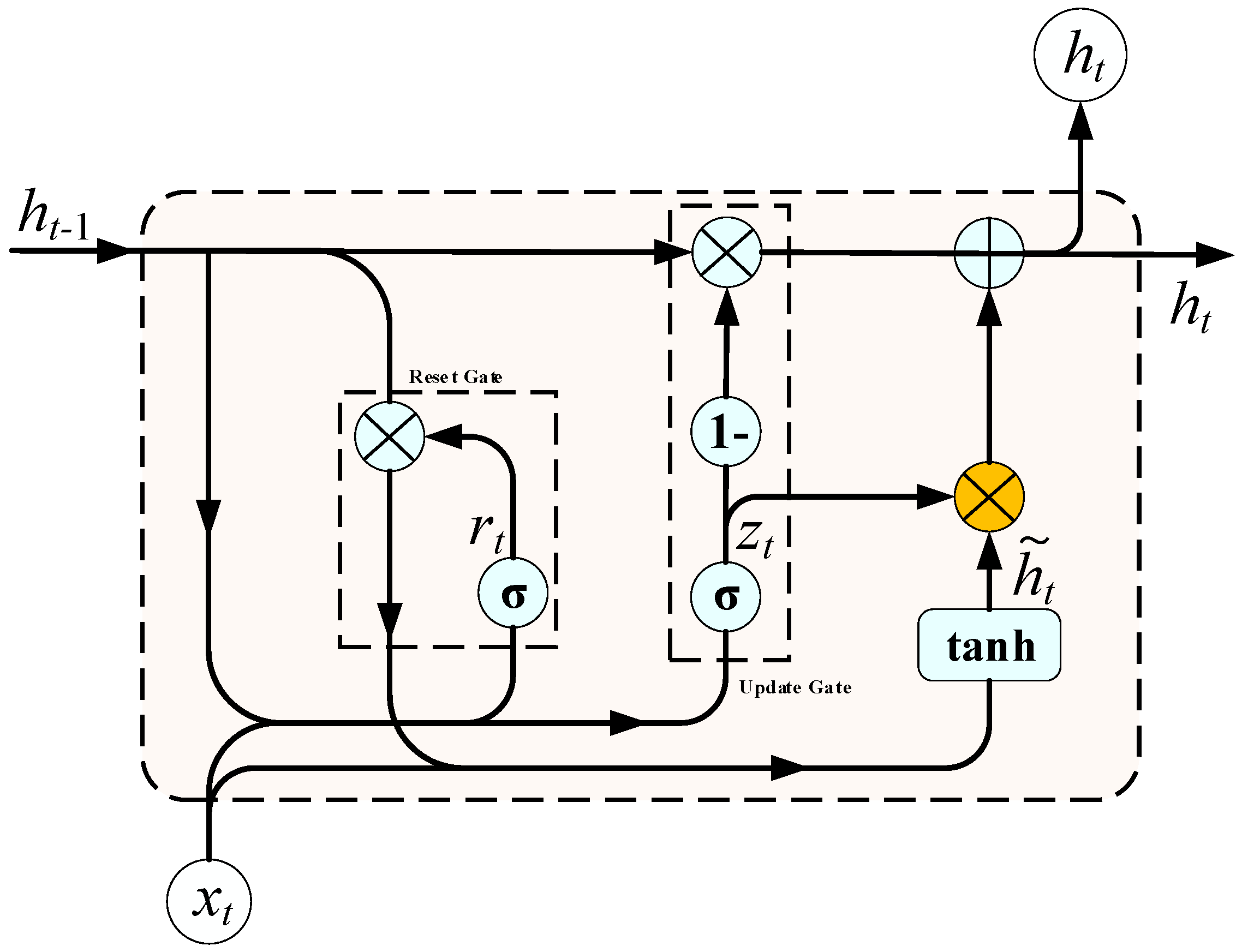
3.1.4. GRU Network
3.2. Model Evaluation Index
4. Result
4.1. Predicted Model Training Results
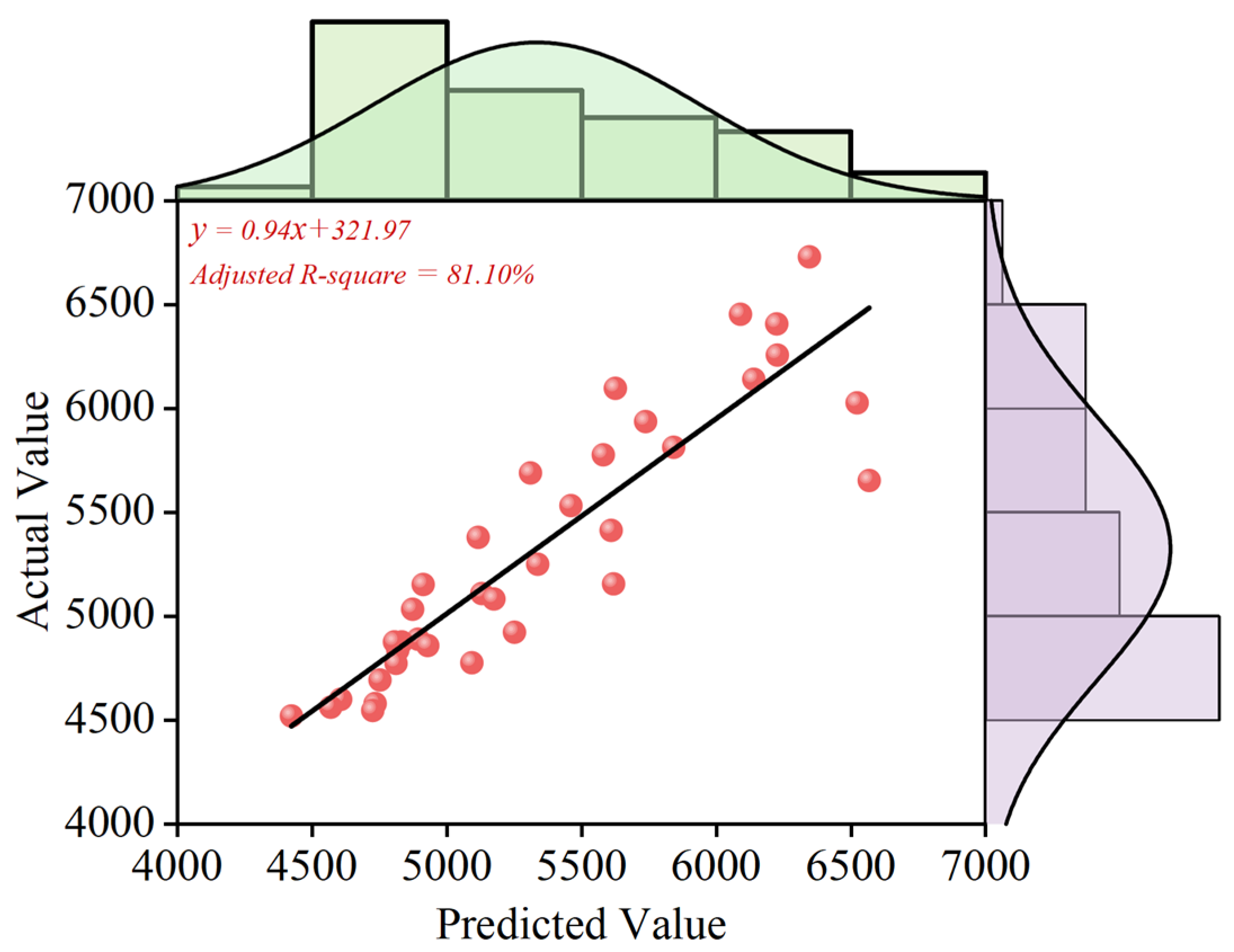
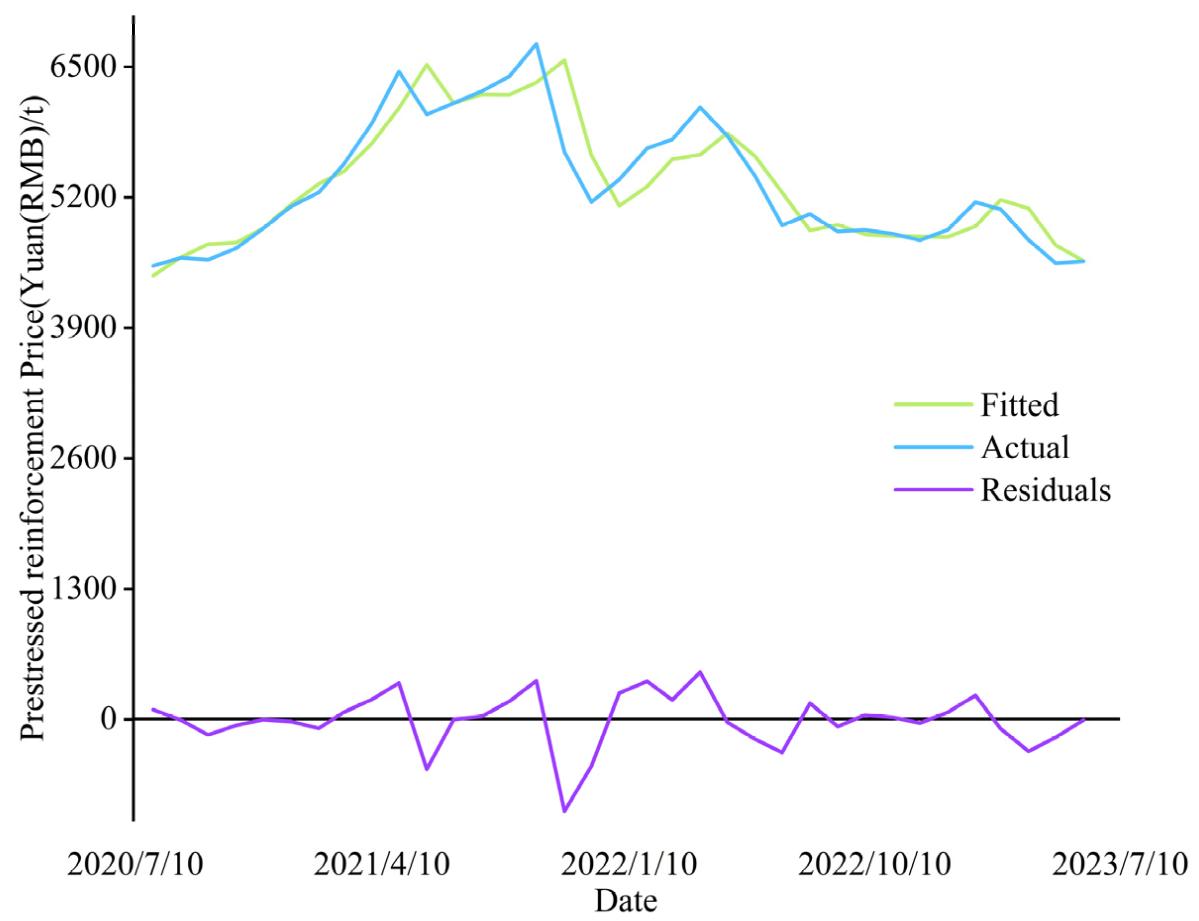
4.2. Results for Verification of Predicted Models
5. Discussion
6. Conclusions
Author Contributions
Funding
Data Availability Statement
Conflicts of Interest
References
- Wang, D.; Liu, J.; Wang, X.; Chen, Y. Cost-effectiveness analysis and evaluation of a ‘three-old’reconstruction project based on smart system. Clust. Comput. 2019, 22, 7895–7905. [Google Scholar] [CrossRef]
- Hwang, S.; Park, M.; Lee, H.-S.; Kim, H. Automated time-series cost forecasting system for construction materials. J. Constr. Eng. Manag. 2012, 138, 1259–1269. [Google Scholar] [CrossRef]
- Marzouk, M.; Hamdala, D. Phasing real estate projects considering profitability and customer satisfaction. Eng. Constr. Archit. Manag. 2024; ahead-of-print. [Google Scholar] [CrossRef]
- Musarat, M.A.; Alaloul, W.S.; Liew, M.; Maqsoom, A.; Qureshi, A.H. Investigating the impact of inflation on building materials prices in construction industry. J. Build. Eng. 2020, 32, 101485. [Google Scholar] [CrossRef]
- Kissi, E.; Sadick, M.; Agyemang, D. Drivers militating against the pricing of sustainable construction materials: The Ghanaian quantity surveyors perspective. Case Stud. Constr. Mater. 2018, 8, 507–516. [Google Scholar] [CrossRef]
- Zhao, C.; Hu, P.; Liu, X.; Lan, X.; Zhang, H. Stock market analysis using time series relational models for stock price prediction. Mathematics 2023, 11, 1130. [Google Scholar] [CrossRef]
- Guo, Z.; Jing, X.; Ling, Y.; Yang, Y.; Jing, N.; Yuan, R.; Liu, Y. Optimized air quality management based on air quality index prediction and air pollutants identification in representative cities in China. Sci. Rep. 2024, 14, 17923. [Google Scholar] [CrossRef]
- Yin, Y.; Shang, P. Forecasting traffic time series with multivariate predicting method. Appl. Math. Comput. 2016, 291, 266–278. [Google Scholar] [CrossRef]
- Mehrmolaei, S.; Savargiv, M.; Keyvanpour, M.R. Hybrid learning-oriented approaches for predicting Covid-19 time series data: A comparative analytical study. Eng. Appl. Artif. Intell. 2023, 126, 106754. [Google Scholar] [CrossRef]
- Tarnate, W.R.D.; Ponci, F.; Monti, A. Uncertainty-aware model predictive control for residential buildings participating in intraday markets. IEEE Access 2022, 10, 7834–7851. [Google Scholar] [CrossRef]
- Uvarova, S.S.; Belyaeva, S.V.; Orlov, A.K.; Kankhva, V.S. Cost Forecasting for Building Materials under Conditions of Uncertainty: Methodology and Practice. Buildings 2023, 13, 2371. [Google Scholar] [CrossRef]
- Jiang, F.; Awaitey, J.; Xie, H. Analysis of construction cost and investment planning using time series data. Sustainability 2022, 14, 1703. [Google Scholar] [CrossRef]
- Ilbeigi, M.; Ashuri, B.; Joukar, A. Time-series analysis for forecasting asphalt-cement price. J. Manag. Eng. 2017, 33, 04016030. [Google Scholar] [CrossRef]
- Kożuch, A.; Cywicka, D.; Adamowicz, K.J.F. A comparison of artificial neural network and time series models for timber price forecasting. Forests 2023, 14, 177. [Google Scholar] [CrossRef]
- Yin, L.; Wang, L.; Li, T.; Lu, S.; Tian, J.; Yin, Z.; Li, X.; Zheng, W. U-Net-LSTM: Time series-enhanced lake boundary prediction model. Land 2023, 12, 1859. [Google Scholar] [CrossRef]
- Yuan, F.; Zhang, Z.; Fang, Z. An effective CNN and Transformer complementary network for medical image segmentation. Pattern Recognit. 2023, 136, 109228. [Google Scholar] [CrossRef]
- de Zarzà i Cubero, I.; de Curtò i Díaz, J.; Roig, G.; Calafate, C.T. LLM Multimodel Traffic Accident Forecasting. Sensors 2023, 23, 9225. [Google Scholar] [CrossRef]
- Tang, B.Q.; Han, J.; Guo, G.-f.; Chen, Y.; Zhang, S. Building material prices forecasting based on least square support vector machine and improved particle swarm optimization. Archit. Eng. Des. Manag. 2019, 15, 196–212. [Google Scholar] [CrossRef]
- Mir, M.; Kabir, H.D.; Nasirzadeh, F.; Khosravi, A. Neural network-based interval forecasting of construction material prices. J. Build. Eng. 2021, 39, 102288. [Google Scholar] [CrossRef]
- Wang, J.; Ashuri, B. Predicting ENR construction cost index using machine-learning algorithms. Int. J. Constr. Educ. Res. 2017, 13, 47–63. [Google Scholar] [CrossRef]
- Liu, Y.; Qin, G.; Huang, X.; Wang, J.; Long, M. Autotimes: Autoregressive time series forecasters via large language models. arXiv 2024, arXiv:2402.02370. [Google Scholar]
- Wang, Y.; Yang, D.; Liu, Y. A real-time look-ahead interpolation algorithm based on Akima curve fitting. Int. J. Mach. Tools Manuf. 2014, 85, 122–130. [Google Scholar] [CrossRef]
- Hamilton, J.D. Why you should never use the Hodrick-Prescott filter. Rev. Econ. Stat. 2018, 100, 831–843. [Google Scholar] [CrossRef]
- Nasir, J.; Aamir, M.; Haq, Z.U.; Khan, S.; Amin, M.Y.; Naeem, M. A new approach for forecasting crude oil prices based on stochastic and deterministic influences of LMD Using ARIMA and LSTM Models. IEEE Access 2023, 11, 14322–14339. [Google Scholar] [CrossRef]
- Jun, W.; Yuyan, L.; Lingyu, T.; Peng, G. A new weighted CEEMDAN-based prediction model: An experimental investigation of decomposition and non-decomposition approaches. Knowl. Based Syst. 2018, 160, 188–199. [Google Scholar] [CrossRef]
- Gao, B.; Huang, X.; Shi, J.; Tai, Y.; Zhang, J. Hourly forecasting of solar irradiance based on CEEMDAN and multi-strategy CNN-LSTM neural networks. Renew. Energy 2020, 162, 1665–1683. [Google Scholar] [CrossRef]
- Shumway, R.H.; Stoffer, D.S. Time Series Analysis and Its Applications (Springer Texts in Statistics); Springer: Berlin/Heidelberg, Germany, 2005. [Google Scholar]
- Thiruchelvam, L.; Dass, S.C.; Asirvadam, V.S.; Daud, H.; Gill, B.S. Determine neighboring region spatial effect on dengue cases using ensemble ARIMA models. Sci. Rep. 2021, 11, 5873. [Google Scholar] [CrossRef]
- Gan, M.; Pan, H.; Chen, Y.; Pan, S. Application of the Variational Mode Decomposition (VMD) method to river tides. Estuar. Coast. Shelf Sci. 2021, 261, 107570. [Google Scholar] [CrossRef]
- Li, X.P.; Shi, Z.-L.; Leung, C.-S.; So, H.C. Sparse index tracking with K-sparsity or ϵ-deviation constraint via ℓ 0-norm minimization. IEEE Trans. Neural Netw. Learn. Syst. 2022, 34, 10930–10943. [Google Scholar] [CrossRef]
- Nazari, M.; Sakhaei, S.M. Successive variational mode decomposition. Signal Process. 2020, 174, 107610. [Google Scholar] [CrossRef]
- Wang, M.-H.; Hung, C. Extension neural network and its applications. Neural Netw. 2003, 16, 779–784. [Google Scholar] [CrossRef]
- Hu, C.; Cheng, F.; Ma, L.; Li, B. State of charge estimation for lithium-ion batteries based on TCN-LSTM neural networks. J. Electrochem. Soc. 2022, 169, 030544. [Google Scholar] [CrossRef]
- Ghazvini, A.; Sharef, N.M.; Sidi, F.B. Prediction of Course Grades in Computer Science Higher Education Program Via a Combination of Loss Functions in LSTM Model. IEEE Access 2024, 12, 30220–30241. [Google Scholar] [CrossRef]
- Gao, S.; Huang, Y.; Zhang, S.; Han, J.; Wang, G.; Zhang, M.; Lin, Q. Short-term runoff prediction with GRU and LSTM networks without requiring time step optimization during sample generation. J. Hydrol. 2020, 589, 125188. [Google Scholar] [CrossRef]
- Xu, M.; Shang, P.; Lin, A. Cross-correlation analysis of stock markets using EMD and EEMD. Phys. A Stat. Mech. Its Appl. 2016, 442, 82–90. [Google Scholar] [CrossRef]
- Huang, Y.; Yu, J.; Dai, X.; Huang, Z.; Li, Y. Air-quality prediction based on the EMD–IPSO–LSTM combination model. Sustainability 2022, 14, 4889. [Google Scholar] [CrossRef]
- Dong, H.; Qi, K.; Chen, X.; Zi, Y.; He, Z.; Li, B. Sifting process of EMD and its application in rolling element bearing fault diagnosis. J. Mech. Sci. Technol. 2009, 23, 2000–2007. [Google Scholar] [CrossRef]
- Ding, J.; Xiao, D.; Huang, L.; Li, X. Gear fault diagnosis based on VMD sample entropy and discrete hopfield neural network. Math. Probl. Eng. 2020, 2020, 8882653. [Google Scholar] [CrossRef]
- Zhang, P.; Gao, D.; Lu, Y.; Kong, L.; Ma, Z. Online chatter detection in milling process based on fast iterative VMD and energy ratio difference. Measurement 2022, 194, 111060. [Google Scholar] [CrossRef]
- Wang, Y.; Chen, P.; Zhao, Y.; Sun, Y. A denoising method for mining cable PD signal based on genetic algorithm optimization of VMD and wavelet threshold. Sensors 2022, 22, 9386. [Google Scholar] [CrossRef]
- Wang, H.; Wu, F.; Zhang, L. Application of variational mode decomposition optimized with improved whale optimization algorithm in bearing failure diagnosis. Alex. Eng. J. 2021, 60, 4689–4699. [Google Scholar] [CrossRef]
- Li, J.; Yao, X.; Wang, H.; Zhang, J. Periodic impulses extraction based on improved adaptive VMD and sparse code shrinkage denoising and its application in rotating machinery fault diagnosis. Mech. Syst. Signal Process. 2019, 126, 568–589. [Google Scholar] [CrossRef]


| Date | Actual | Predicted | Residuals |
|---|---|---|---|
| 2020-8-1 | 3520.00 | 4422.52 | 97.47 |
| 2020-9-1 | 4600.00 | 4606.04 | −6.04 |
| 2020-10-1 | 4590.00 | 4738.86 | −153.86 |
| 2020-11-1 | 4693.00 | 4750.98 | 57.98 |
| 2020-12-1 | 4890.00 | 4892.68 | −2.68 |
| 2021-1-1 | 5110.00 | 5128.93 | −18.93 |
| 2021-2-1 | 5500.00 | 5337.11 | −87.11 |
| 2021-3-1 | 5533.00 | 5459.93 | −126.66 |
| 2021-4-1 | 5640.00 | 5571.37 | 199.04 |
| 2021-5-1 | 6433.33 | 6069.67 | 363.66 |
| 2021-6-1 | 5666.67 | 6522.55 | −255.88 |
| 2021-7-1 | 5540.00 | 6139.05 | −199.05 |
| 2021-8-1 | 6256.67 | 5645.58 | 611.10 |
| 2021-9-1 | 6400.00 | 6206.27 | 193.73 |
| 2021-10-1 | 6730.00 | 6345.15 | 384.85 |
| 2021-11-1 | 6563.33 | 6587.06 | −313.73 |
| 2021-12-1 | 6155.82 | 6618.85 | −463.03 |
| 2022-1-1 | 5880.11 | 5966.36 | −86.25 |
| 2022-2-1 | 5690.00 | 5897.80 | 380.20 |
| 2022-3-1 | 5776.67 | 5580.46 | 196.21 |
| 2022-4-1 | 6066.67 | 5625.06 | −71.61 |
| 2022-5-1 | 5813.33 | 5841.02 | −27.69 |
| 2022-6-1 | 4923.33 | 5119.30 | −195.98 |
| 2022-7-1 | 4923.33 | 5250.18 | −326.85 |
| 2022-8-1 | 5033.33 | 4872.65 | 160.68 |
| 2022-9-1 | 4860.00 | 4928.97 | −68.97 |
| 2022-10-1 | 4476.67 | 4625.76 | −149.09 |
| 2022-11-1 | 4437.94 | 4417.82 | 20.13 |
| 2022-12-1 | 4774.15 | 4810.37 | −36.22 |
| 2023-1-1 | 4478.33 | 4505.79 | 70.54 |
| 2023-2-1 | 5153.33 | 4422.20 | −21.13 |
| 2023-3-1 | 5087.88 | 4374.26 | 378.09 |
| 2023-4-1 | 4776.67 | 4092.53 | −315.86 |
| 2023-5-1 | 4486.67 | 4308.58 | 178.09 |
| 2023-6-1 | 4563.33 | 4568.98 | −5.65 |
| Evaluation Metrics | Adjusted R-Squared Value | MSE | MAE | RMSE |
|---|---|---|---|---|
| ARIMA | 78.80% | 90,420.24 | 200.60 | 300.70 |
| LSTM | 75.00% | 101,296.81 | 253.02 | 318.20 |
| CNN-LSTM | 38.30% | 169,337.18 | 307.13 | 411.50 |
| TCN | 73.10% | 100,996.78 | 258.86 | 317.80 |
| CEEMDAN-VMD-GRU-ARIMA | 81.10% | 73,078.79 | 189.39 | 270.33 |
Disclaimer/Publisher’s Note: The statements, opinions and data contained in all publications are solely those of the individual author(s) and contributor(s) and not of MDPI and/or the editor(s). MDPI and/or the editor(s) disclaim responsibility for any injury to people or property resulting from any ideas, methods, instructions or products referred to in the content. |
© 2025 by the authors. Licensee MDPI, Basel, Switzerland. This article is an open access article distributed under the terms and conditions of the Creative Commons Attribution (CC BY) license (https://creativecommons.org/licenses/by/4.0/).
Share and Cite
Guo, Z.; Luo, Y.; Yi, T.; Jing, X.; Ma, J. Harnessing the Power of Improved Deep Learning for Precise Building Material Price Predictions. Buildings 2025, 15, 873. https://doi.org/10.3390/buildings15060873
Guo Z, Luo Y, Yi T, Jing X, Ma J. Harnessing the Power of Improved Deep Learning for Precise Building Material Price Predictions. Buildings. 2025; 15(6):873. https://doi.org/10.3390/buildings15060873
Chicago/Turabian StyleGuo, Zhilong, Yayong Luo, Tongqiang Yi, Xiangnan Jing, and Jing Ma. 2025. "Harnessing the Power of Improved Deep Learning for Precise Building Material Price Predictions" Buildings 15, no. 6: 873. https://doi.org/10.3390/buildings15060873
APA StyleGuo, Z., Luo, Y., Yi, T., Jing, X., & Ma, J. (2025). Harnessing the Power of Improved Deep Learning for Precise Building Material Price Predictions. Buildings, 15(6), 873. https://doi.org/10.3390/buildings15060873