A New Prediction Model of Dam Deformation and Successful Application

Abstract

In most dam deformation monitoring practices, some single-point models do not consider the spatial correlation, and the traditional regression models do not consider the nonlinear relationship between the environmental quantity and the deformation quantity, resulting in poor prediction accuracy. In view of the poor accuracy of the monitoring data, which reflect the overall deformation response in the current dam monitoring practices, this paper proposes an innovative solution of ensemble empirical mode decomposition and a wavelet noise reduction method. A high-precision prediction model considering spatial correlation is constructed. By studying the measured deformation data of an arch dam and comparing the performance parameters of various models, the superiority and universality of the proposed method are verified. Dam deformation monitoring data are of great significance to describe the operation behavior of dams. It is significant for us to optimize the health monitoring of dam safety structures and ensure dam safety and realize social harmony in our country.

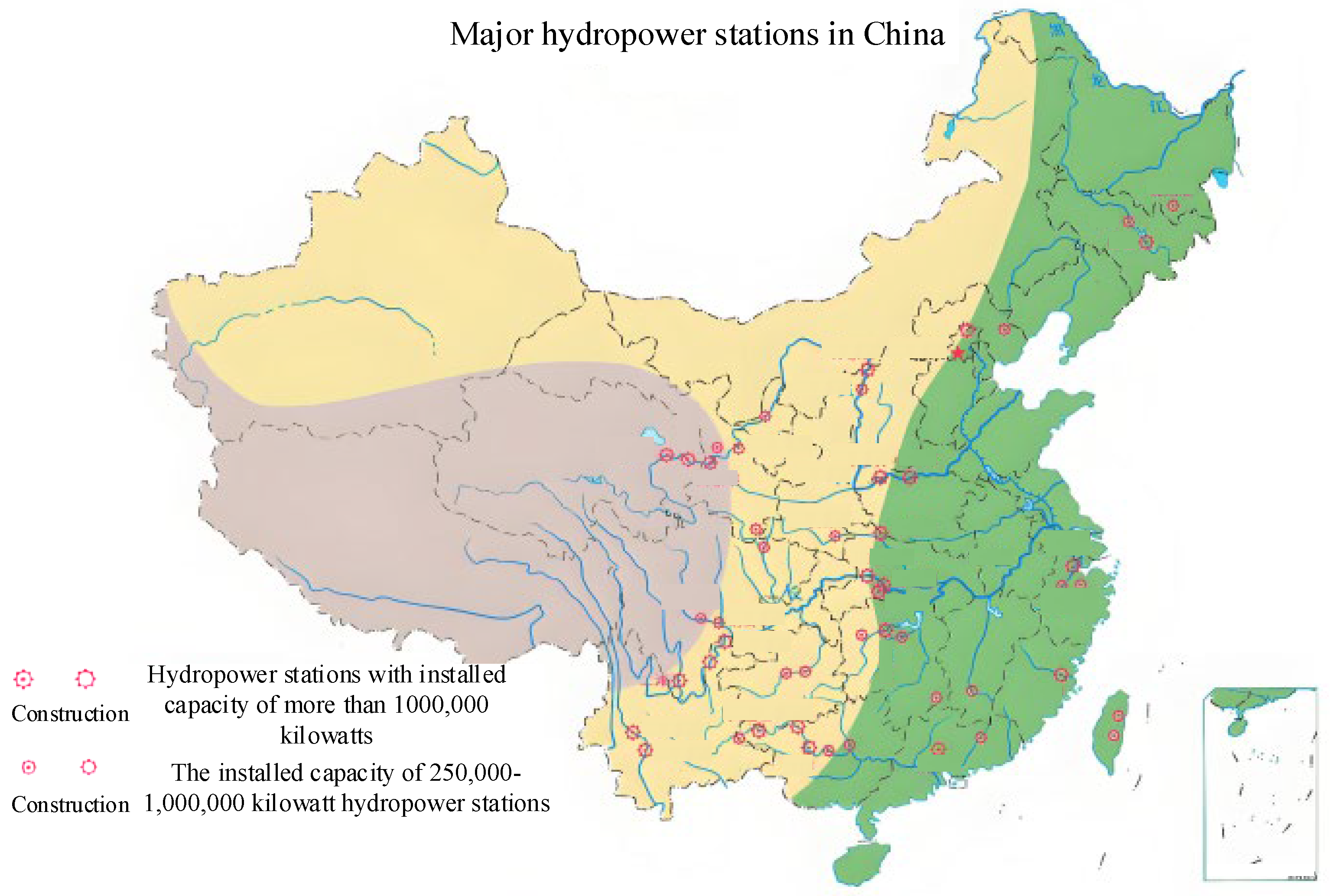
1. Introduction

As an important civil infrastructure, dams have made great contributions to regional social and economic development by continuously providing seasonal water sources or generating renewable energy. There are approximately 58,000 such large dams (more than 15 m high) worldwide with an estimated cumulative storage capacity of between 7000 and 8300 km³ [1]. Dams, especially high dams, provide many benefits, including flood control, water supply, and power generation. However, if a dam breaks, unfortunately, it will also bring a devastating blow to people’s lives and property safety [2]. Dam safety prediction and early warning are the core links to ensure the safe operation of dams. With the continuous development of computer technology, advanced machine learning algorithms have shown more and more advantages in dam safety prediction analysis. However, the accuracy of traditional dam deformation prediction models is low, which will seriously affect the assessment of dam safety states. Therefore, new methods and technologies are needed to improve the accuracy and generalization ability of dam deformation prediction and overcome the challenges from many external extreme natural conditions, dam body defects, and potential risks in safe operation [3,4,5]. At present, there is a contradiction between the demand and the reality of dam safety monitoring and risk analysis ability. How to understand and solve these contradictions needs to be explored from the source of philosophical thinking. In the understanding and practice of dam safety monitoring, we should consciously take the theory of practice, epistemology, and contradiction as guidance and explore the philosophical roots of dam safety monitoring and risk analysis practice from the perspectives of connection and development. 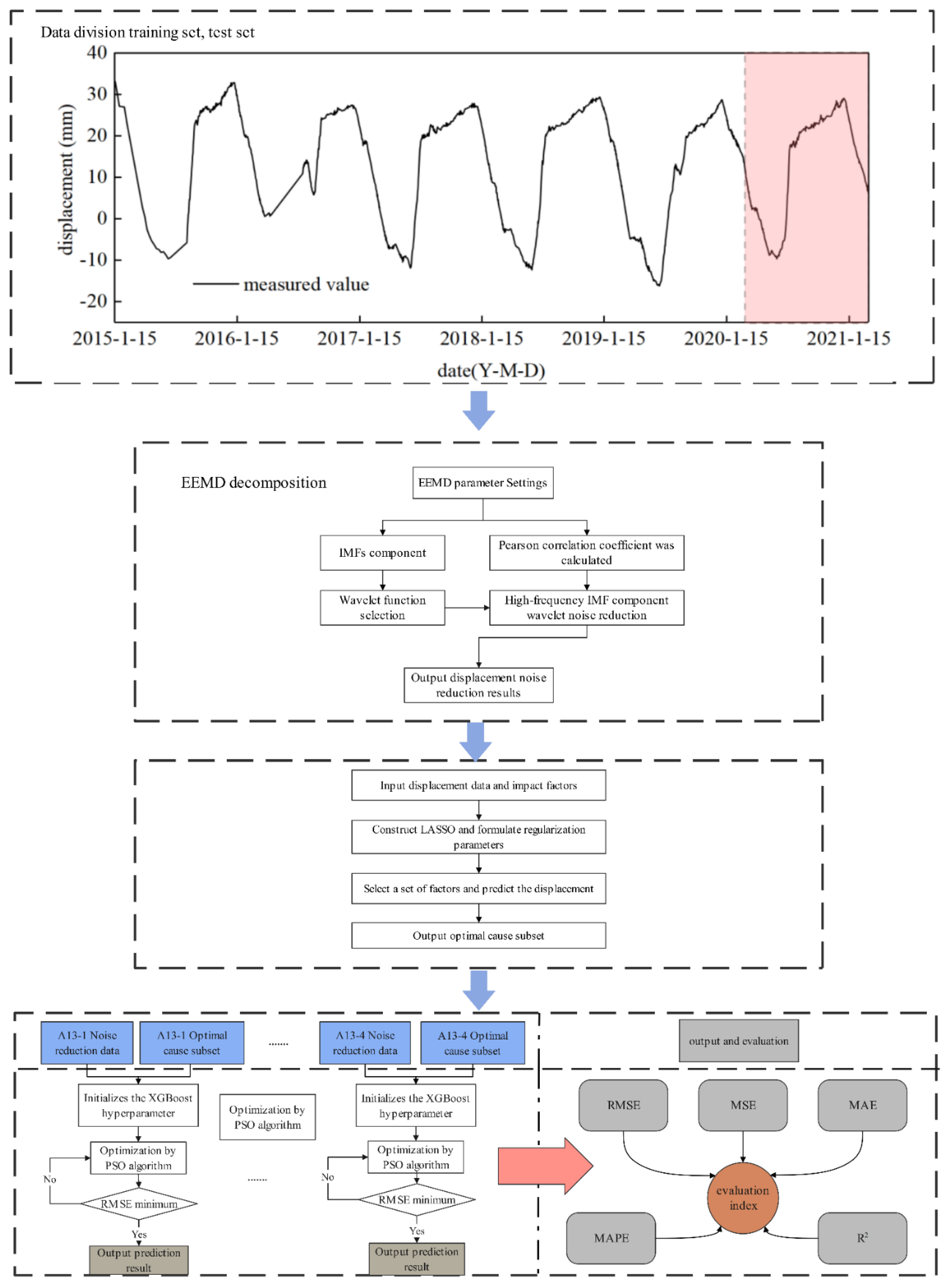This is of great significance for us to establish a dam safety monitoring system that is compatible with the level of economic development and to construct a reasonable dam safety monitoring risk evaluation index system (Figure 1).

2. Theory and Method

As an important water retaining structure in water conservancy projects, a dam has the characteristic of raising the water level. By 2020, China will have 4872 large- and medium-sized reservoirs with a total storage capacity of 858.9 billion cubic meters. Dam displacement can effectively reflect their operating state and is an important index of dam safety structure health monitoring. It is of great significance to establish an accurate and reliable displacement prediction model for dam health monitoring. Based on the above-mentioned philosophical thinking on contradiction theory, practice theory, epistemology, and system theory and aiming at problems such as the low prediction accuracy of the current analysis model and the insufficient depth of data mining, this paper proposes a dam displacement analysis and prediction model. By using variational mode decomposition of the original deformation sequence data to obtain the components in different frequency domains, an EEMD–wavelet data denoising model was established, and a nonlinear intelligent optimization algorithm was adopted considering the spatio-temporal correlation of multiple measurement points. A spatio-temporal prediction model based on the EEMD–wavelet model was proposed. The accuracy and precision of the prediction model are improved under this prediction model.

Some scholars, including Xu Ren, used the more common LSTM model and intelligent optimization algorithm, and they fully considered the temporal correlation of measurement point data but did not consider the characteristics of the spatial distribution of dam measurement points. Referring to the spatial model proposed by Wu ZhongRu [2], there is a large number of factors involved in his model, in which the subsets of factors affecting the displacement of dams are fully considered. However, the establishment of a dam displacement prediction model faces a problem of balance. If too many influencing factors are considered, the model may perform well in one case but fail to adapt to others, called “overfitting”. On the contrary, when processing long time-series data, the model needs to maintain computational efficiency and accuracy while ensuring appropriate generalization ability [3,4,5].

In recent years, artificial intelligence algorithms have been widely used in the field of dam displacement prediction, which is mainly divided into traditional regression models and machine learning algorithms [6,7]. The predictive methods include the multivariate linear model and generalized linear model, but in these methods, some problems remain to be solved. Neural network algorithms, including BP (back propagation), RBF (radial basis function) neural networks, and GBDTs (gradient lifting decision trees), can better mine the nonlinear relationship in the dam displacement data and make predictions. These algorithms can be combined with intelligent algorithms and optimization algorithms to optimize the hyperparameters of deep learning algorithms for faster and more accurate predictions.

Xu [8] studied and discussed the application of XGBoost in the displacement prediction of concrete dams and achieved good prediction results based on the data of a single measurement point. Zhou et al. [9] adopted the LSTM neural network prediction algorithm based on SSA to pre-process the original data into trend terms and periodic terms and then used them in LSTM and GF algorithms to make full use of the timing of the data. Qi [10] screened the subsets of influence factors of dam deformation and built a dam deformation analysis model based on LSTM. Wu et al. [11] clustered the original data, combined with the WOA of whale behavior habits in nature to optimize LSSVM’s hyperparameter selection, and achieved a good prediction effect. Dong Yong [12] extracted the effective information of dam deformation through empirical mode decomposition in signal processing and, finally, adopted LSTM as the prediction model.

Although the above models take into account the temporal and spatial correlations of the measuring points, which can improve the prediction effect to a certain extent, most of them are multi-measuring point models based on statistics, and there are still the following problems: (1) In the regression analysis, the determination of a large number of constants may lead to infinite or no solutions to linear equations, so factor screening is required to reduce the impact of low model generalization [13,14]. (2) There is a nonlinear relationship between the environmental factors of a dam, and there is a nonlinear mapping between the environmental quantity and the displacement data. (3) Affected by various factors, noise exists in dam displacement, environment, and temperature data [15,16], which affects the prediction accuracy. To solve the problem, a nonlinear intelligent optimization algorithm based on EEMD–wavelet data denoising was established, and a spatio-temporal prediction model based on the EEMD–wavelet model was proposed. A concrete arch dam in the lower Yalong River was taken as an example to verify the accuracy of the model.

2.1. Basic Principle of Statistical Model for Dam Deformation Prediction

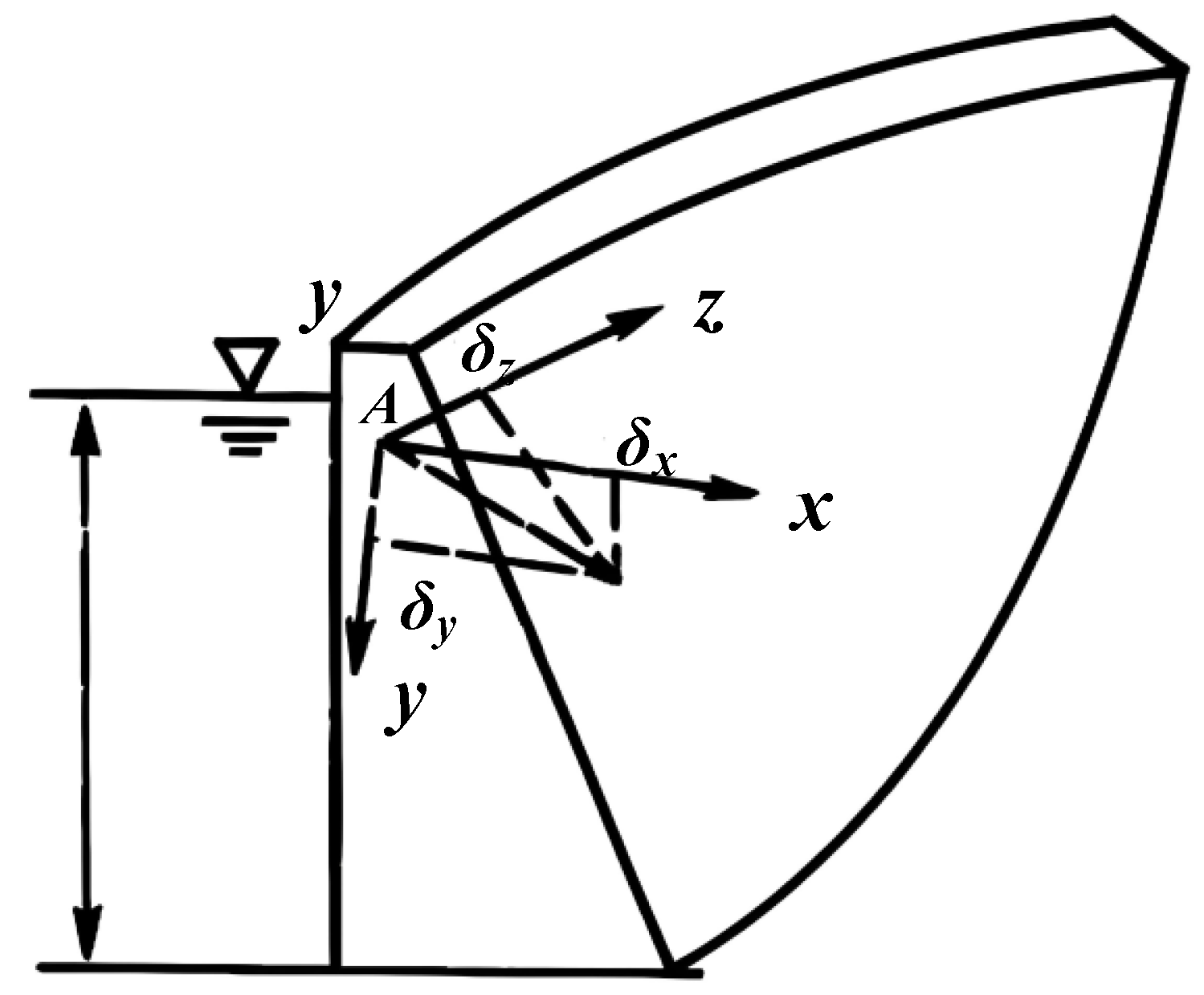
According to the existing dam safety monitoring theory and the calculation of material mechanics and structural mechanics (Figure 2), the displacement at any point of a concrete dam under the influence of hydrostatic pressure, lifting pressure, temperature, aging, etc., can be expressed as the following equation [17]:

$$\left({\delta }_x,{\delta }_y,{\delta }_z\right)={\delta }_W+{\delta }_T+{\delta }_{\theta }$$

(1)

where ${\delta }_x$, ${\delta }_y$, and ${\delta }_z$, respectively, refer to the displacement in xyz directions of the dam body; according to its cause, the displacement can be divided into three parts: water pressure component (${\delta }_W$), temperature component (${\delta }_T$), and aging component (${\delta }_{\theta }$).

Under the action of water pressure, the horizontal displacement produced by any observation point of the dam is composed of three parts: the displacement caused by the internal force of the reservoir water pressure acting on the dam body; the displacement caused by the deformation of the foundation caused by the internal force on the foundation; and the displacement caused by the rotation of foundation surface due to the heavy action of reservoir water. Through the calculation of water pressure and water pressure components using the mechanical method, it can be concluded that the water pressure component ${\delta }_{\theta }$ and the water depth ${\delta }_{\theta }$ (i = 1, 2, … n power degree) form a linear relationship, that is:

$${\delta }_W={\displaystyle \sum _{i=1}^n{a}_i{H}^i}$$

(2)

where $a_i$ is the coefficient; $H$ is the water depth in front of the dam; and $n$ is the highest degree of the polynomial, where the gravity dam $n$ takes a value of 3.

The temperature component is mainly due to the displacement caused by the temperature change in the concrete and bedrock of the dam body. When enough thermometer data are accurately recorded, the temperature component can be calculated using the measured temperature, and the prediction model established is the Hydrostatic-Thermal-Time model, referred to as the HTT [18] model, as follows:

$${\delta }_T={\displaystyle \sum _{i=1}^m{b}_i}{T}_i$$

(3)

where b is the statistical coefficient, m is the effective temperature count, and T is the measured temperature.

However, when the temperature monitoring data in the dam are insufficient, the Hydrostatic-Seasonal-Time model (HST model for short) can be used:

$${\delta }_T={\displaystyle \sum _{i=1}^2\left(b_{i,1}\left(\sin \frac{2\mathrm{\pi }it}{365}-\sin \frac{2\mathrm{\pi }i{t}_0}{365}\right)\right)}+{\displaystyle \sum _{i=1}^2\left(b_{i,2}\left(\cos \frac{2\mathrm{\pi }it}{365}-\cos \frac{2\mathrm{\pi }i{t}_0}{365}\right)\right)}$$

(4)

where b is the regression coefficient, and t is the cumulative number of days from the monitoring date to the first measurement date.

The aging factor is the synthesis of many nonlinear factors, and its influence on the response eventually manifests in the development of a certain direction with the continuous extension of time. As a material entity, the dam’s movement changes in time and space. Time signifies the continuity and sequence of material movement, characterized by one dimension, while space is the extensiveness of material movement, characterized by three dimensions. The time and space of material movement are inseparable, which requires us to do things according to a specific time and place and conditions.

The generation of dam aging components is caused by many complicated factors. It comprehensively reflects the creep and plastic deformation of concrete and bedrock and the compressive deformation of the geological structure of bedrock. Generally speaking, the aging displacement of dams in normal operation changes rapidly in the initial stage and slows down gradually in the later stage. The aging component can be modeled using a variety of mathematical models. For the aging component of concrete dam during its service life, the linear combination form of $\theta$ and $\ln \theta$ is used, that is

$${\delta }_{\theta }=c_1\theta +c_2\ln \theta$$

(5)

where $\theta$ is $\theta ={\displaystyle \frac{t}{100}}$; $t$ the number of days from the monitoring date to the beginning of the measurement date; and $c_1$ and $c_2$ are the coefficients.

In summary, the HST model can be obtained from the analysis of displacement components at any point of the dam:

$$\begin{array}{l}\delta ={\delta }_W\left(t\right)+{\delta }_T\left(t\right)+{\delta }_{\theta }\left(t\right)\\ =a_0+{\displaystyle \sum _{i=1}^{3\left(4\right)}{a}_i\left(H_i-H_{i,0}\right)}+{\displaystyle \sum _{i=1}^2\left(b_{i,1}\left(\sin \frac{2\mathrm{\pi }it}{365}-\sin \frac{2\mathrm{\pi }i{t}_0}{365}\right)\right)}\\ +{\displaystyle \sum _{i=1}^2\left(b_{i,2}\left(\cos \frac{2\mathrm{\pi }it}{365}-\cos \frac{2\mathrm{\pi }i{t}_0}{365}\right)\right)}+c_1\left(\theta -{\theta }_0\right)\\ +c_2\left(\ln \theta -\ln {\theta }_0\right)\end{array}$$

(6)

The meaning of each symbol in Formula (6) is the same as that of Formulas (1)–(5).

Dam deformation monitoring is inseparable from time- and space-influencing factors. The above equation describes the deformation law of a concrete dam with a single measuring point and only considers the time factor, so it is difficult to describe the spatial correlation of multiple measuring points. On the basis of the above formula, space coordinates are introduced. Each term is expanded according to multiple power series, and with reference to the beam deflection line equation of engineering mechanics, the following results are obtained:

$$\begin{array}{l}\delta ={\displaystyle \sum _{k=0}^{3(4)}{\displaystyle \sum _{n=0}^3{A}_{kn}}}{H}^k{z}^n+\\ {\displaystyle \sum _{j,k=0}^1{\displaystyle \sum _{n=0}^3{B}_{jkn}}}\sin ({\displaystyle \frac{2\pi jt}{365}})\cdot \cos ({\displaystyle \frac{2\pi kt}{365}})z^n+\\ {\displaystyle \sum _{j,k=0}^1{\displaystyle \sum _{n=0}^3{C}_{jkn}}}{\theta }_j\cdot \ln {\theta }_k{z}^n\end{array}$$

(7)

2.2. PSO (Particle Swarm) Algorithm

The PSO algorithm is derived from the research on the foraging behaviors of birds [19] and is a swarm intelligence algorithm for solving optimization problems. In the algorithm, each particle has two basic properties: position and velocity. The position represents the potential solution of the optimization problem and corresponds to the fitness value of each particle after the fitness function is calculated. The speed of the particle will be dynamically adjusted and updated in each iteration along with the extreme value of the particle itself and the global particle, so as to determine the movement direction and distance of the particle in the next iteration step. The specific updated formula is as follows:

$$\begin{array}{c}{v}_{id}^{(k+1)}=w{v}_{id}^{(k)}+s_1{r}_1\left(P_{id}^{(k)}-X_{id}^{(k)}\right)+s_2{r}_2\left(P_{gd}^{(k)}-X_{id}^{(k)}\right)\\ X_{id}^{(k+1)}=X_{id}^{(k)}+v_{id}^{(k+1)}\end{array}$$

(8)

where $v_{id}^{(k+1)}$, $X_{id}^{(k)}$, and $P_{id}^{(k)}$ are, respectively, the velocity, position, and individual extremum of particle i after the KTH iteration in the D-dimensional search space; $P_{gd}^{(k)}$ is the global extreme value of the population after the KTH iteration in the D-dimensional search space; $s_1$ and $s_2$ are non-negative acceleration factors; $r_1$ and $r_2$ are random numbers between [0, 1]; and $w$ is the inertia weight. After several iterations, parameter optimization in the solvable space can be realized (Figure 3).

The PSO algorithm has a simple principle [20], fast convergence speed, and strong versatility. However, when the data re more complex, the dimension is higher, and the parameters are not set properly, problems such as premature convergence, low search accuracy, and low late iteration efficiency easily occur. With the progress of iteration, the algorithm gradually shifts from the global search stage to the local search stage. Different stages have different requirements for the algorithm optimization ability. In the early stage, the search scope is large, and it is necessary to pay attention to diversity while improving the search efficiency. And in the later stage, more attention should be paid to the convergence ability of the algorithm. Meanwhile, the loss of diversity should also be reduced to avoid premature convergence of the algorithm. The dynamic adjustment of $w$ can make the PSO algorithm achieve better optimization results at each stage. In this paper, linear decreasing inertia weights are selected to better balance the global search and local search capabilities of the algorithm. The expression is as follows:

$$w_k=w_1-\left(w_1-w_2\right)k/k_{\max }$$

(9)

where k is the number of current iterations; k_max is the maximum number of iterations; $w_k$ is the inertia weight for the K iteration time; and $w_1$ and $w_2$ are the initial and end values of the inertia weights, respectively.

In the iterative process, the PSO algorithm [21,22] may fall into the local extreme value due to the fast convergence speed and, thus, converge prematurely. In order to solve the problem of premature convergence, the mutation operation of the genetic algorithm is introduced; that is, the particle position is initialized with a certain probability during each iteration, so that some particles jump out of the local optimal position previously searched and re-search in a larger range.

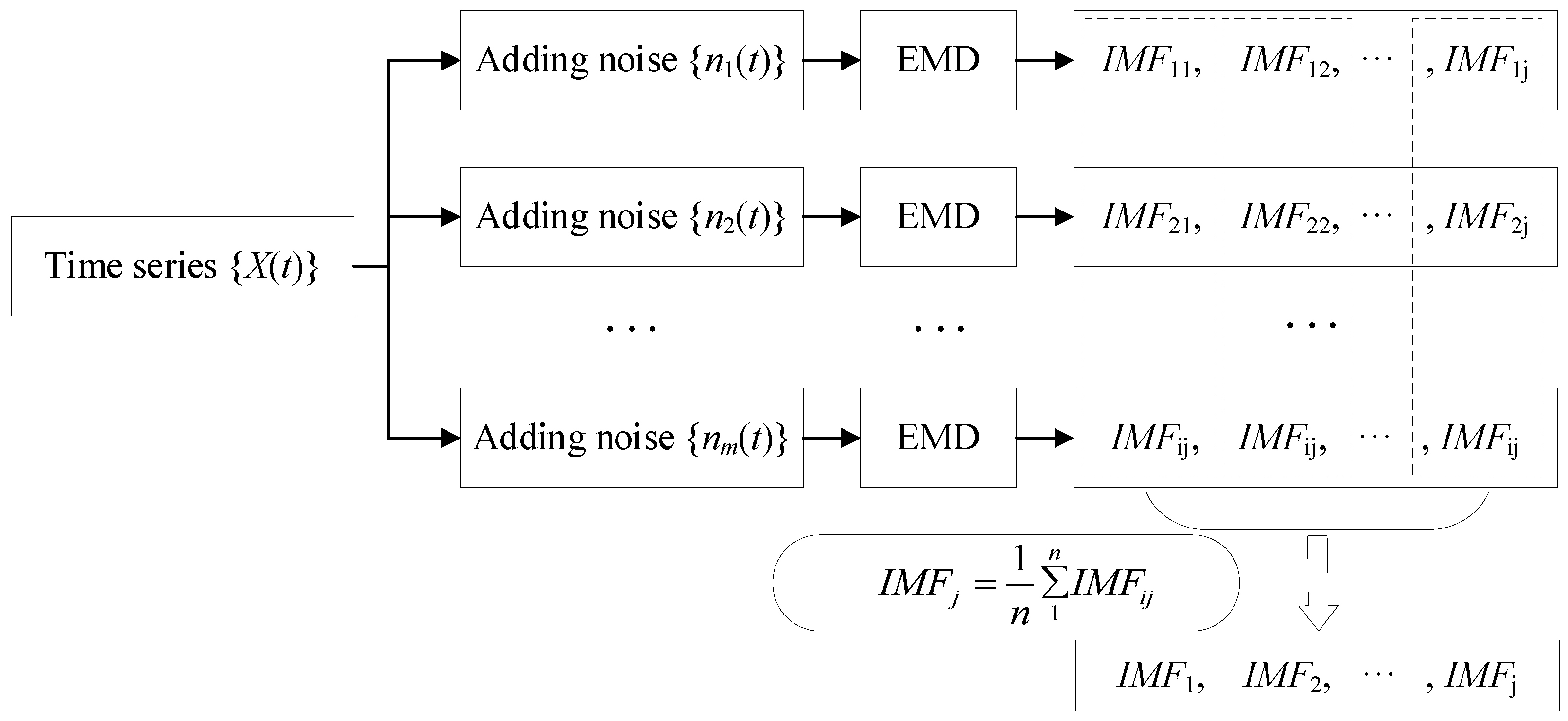
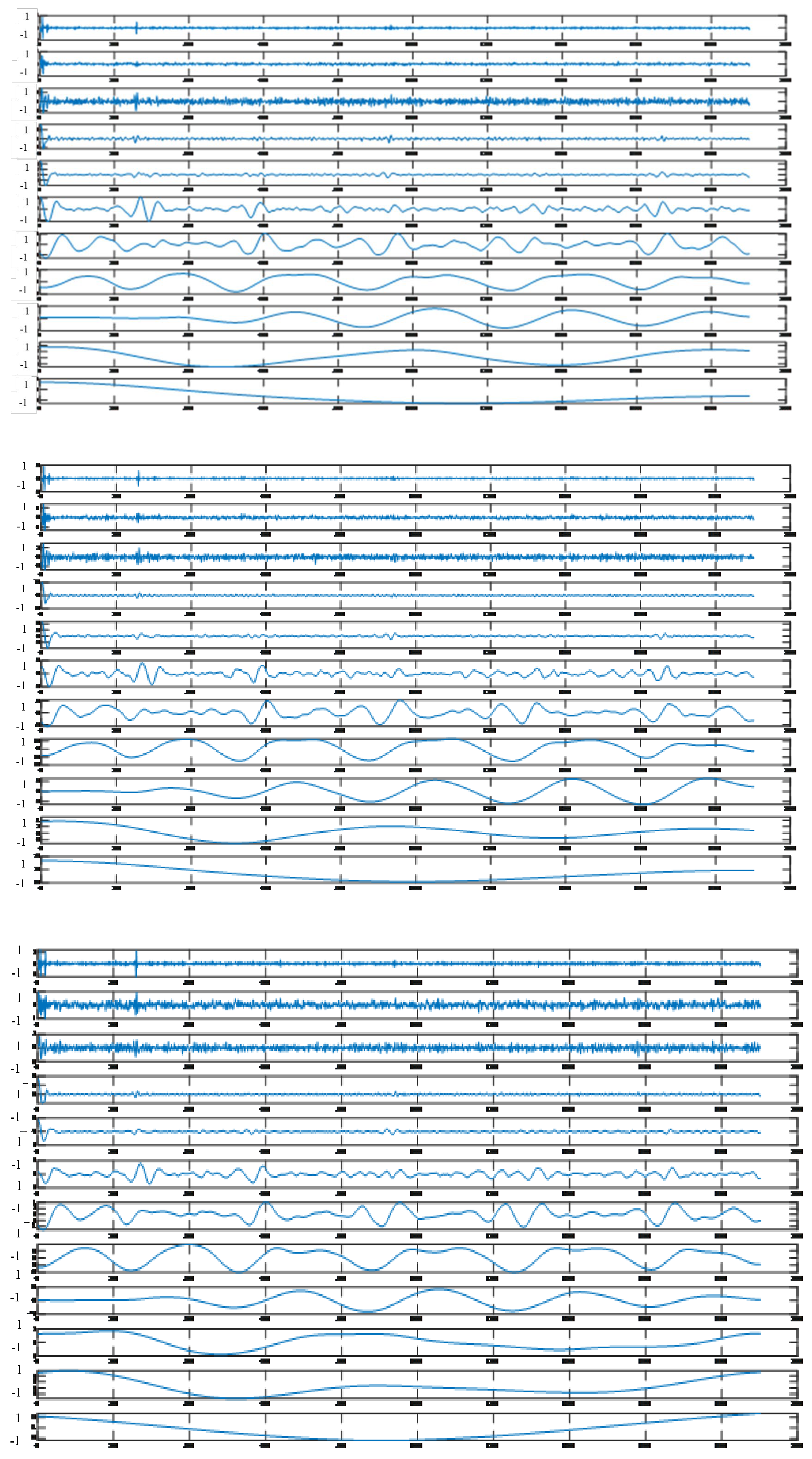
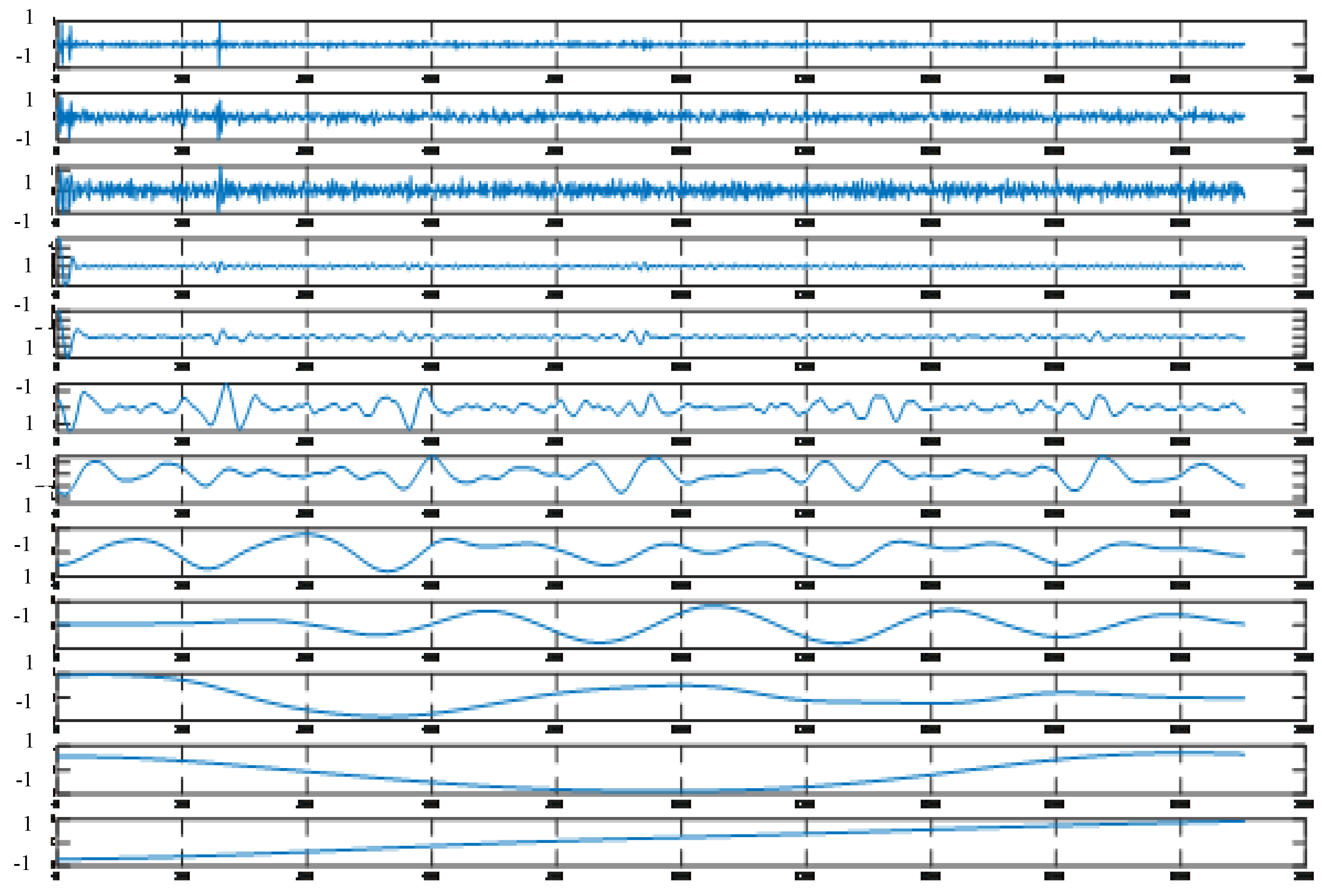
2.3. EEMD and Wavelet Noise Reduction Principle

2.3.1. Principles of EEMD

EEMD is an improved model of empirical mode decomposition (EMD) [23]. Huang et al. believe that any original signal is composed of several overlapping eigenmode functions. In essence, EMD stabilizes the signal to obtain a series of IMFs with a gradually stable frequency and a margin B. However, when the time scale of the signal has a jump change, IMFs will contain different time-scale feature components, and EMD itself has the disadvantage of being prone to modal confusion. For these situations, Huang and Wu proposed the EEMD model. By adding white noise to the signal to be decomposed, EEMD utilizes the uniform distribution of the white noise spectrum to make the original signal spread over the white noise background with a uniform distribution in the entire time–frequency space, and the signals of different time scales will be automatically distributed on the appropriate reference scale, making the signals have continuity at different scales, thus achieving the purpose of suppressing mode confusion. Since the mean value of white noise is zero, after adding white noise several times and obtaining the average value, the additional noise is eliminated, and the result is the signal itself.

The EEMD steps are as follows (Figure 4):

Step 1: The noise series $n_m(t)$ is added to the time series $\left\{X(t)\right\}$ of the dam observation data to obtain the time series $\left\{X_m(t)\right\}$ of adding noise:

$$X_m(t)=X(t)+n_m(t)$$

(10)

where $n_m(t)$ is the amplitude $\alpha$.

Step 2: The time series $X_m(t)$ obtained in step 1 is decomposed using EEMD into a series of IMFs and a margin B.

Step 3: Step 1 and Step 2 are repeated n times. The jth-order IMF after the ith EMD is represented by IMF_ij, and the margin B after the ith EMD is represented by B_i.

Step 4: All IMFs of the same order and all allowances B are averaged to obtain the final IMF_j of each order and allowance B:

$$IM{F}_j={\displaystyle \frac{1}{n}}\sum _1^{n}IM{F}_{ij}$$

(11)

where j is the order of the partition, and i is the number of EMDs performed on the time series.

$$B={\displaystyle \frac{1}{n}}\sum _1^n{B}_i$$

(12)

When performing EEMD, the added white noise, $\alpha$ amplitude, and repetition times $n$ need to be determined after several experiments. The value pointed out by Chen Zhong is usually 0.01~0.5, and the value of repetition times $n$ is usually 100~200 times.

2.3.2. High-Frequency Signal Test

After the original signal is decomposed via EEMD [24], it is necessary to calculate the correlation between the generated components IMF and the original data in order to carry out wavelet packet noise reduction. The correlation coefficient C_k formula is as follows:

$$C_k={\displaystyle \frac{{\displaystyle \sum \left(y\left(n\right)-\overline{y\left(n\right)}\right)\left(y^{\prime }\left(n\right)-\overline{y^{\prime }\left(n\right)}\right)}}{\sqrt{{{\displaystyle \sum \left(y\left(n\right)-\overline{y\left(n\right)}\right)}}^2{{\displaystyle \sum \left(y^{\prime }\left(n\right)-\overline{y^{\prime }\left(n\right)}\right)}}^2}}}$$

(13)

where $y^{\text{'}}(n)$ is a certain IMF component, $y(n)$ is the original data, and $\overline{y(n)}$ and $\overline{y^{\text{'}}(n)}$ are the average values. When the calculated value C_k is above 0.3, the correlation can be considered high. Otherwise, the component IMF has poor correlation with the original data.

2.3.3. Wavelet Noise Reduction

Dam deformation monitoring data can be regarded as a kind of signal, which is usually disturbed by noise caused by random factors and observation errors from complex environments. In order to extract useful information from these signals to characterize the detected object and improve the accuracy of the data, it is necessary to process the data by denoising them. Wavelet analysis is a method for time–frequency analysis of signals, which gradually developed from the field of signals in the late 1980s. Compared with the single resolution of Fourier transform, wavelet analysis has the characteristics of multi-resolution analysis, so it is widely used in the signal denoising [25] field. For the dam deformation observation signal s(n) containing noise, it can be expressed as follows:

$$s(n)=f(n)+\sigma \cdot e(n)$$

(14)

where $s(n)$ is the signal containing noise; and $f(n)$ is a useful signal. The essence of wavelet denoising is that an approximation signal $f^{\text{'}}(n)$ obtained from a noisy signal $s(n)$ is the optimal approximation to $f(n)$ under a certain error; that is, the actual signal is separated from the noisy signal to the maximum extent, the real signal is retained, and the noise signal is removed so as to achieve the purpose of denoising. Nowadays, there are two kinds of wavelet denoising methods commonly used: hard threshold denoising and soft threshold denoising. Because hard threshold denoising will eliminate some useful signals that are not noise and cause signal distortion, this paper adopts soft threshold denoising (Figure 5).

2.3.4. Noise Reduction Evaluation Indicators

In signal processing, noise reduction evaluation indexes are mainly measured by smoothness ($r$) and the noise reduction error ratio ($dnSNR$). The larger the noise reduction error ratio, the smaller the smoothness, indicating that the algorithm has better noise reduction effect, and the noise reduction effect directly affects the prediction accuracy of the prediction model.

The smoothness of the curve $r$ after noise reduction is as follows:

$$r={\displaystyle \frac{{{\displaystyle {\sum }_{t=1}^{N-1}\left[x^{\text{'}}(t+1)-x^{\text{'}}(t)\right]}}^2}{{{\displaystyle {\sum }_{t=1}^{N-1}\left[x(t+1)-x(t)\right]}}^2}}$$

(15)

The calculation formula of the noise reduction error ratio is as follows:

$$\left\{\begin{array}{l}dnSNR=10\lg (p_{s+n}/p_n)\\ p_{s+n}={\displaystyle {\sum }_{t=1}^N{x}^2(t)}\\ p_n={{\displaystyle {\sum }_{t=1}^N\left[x(t)-x^{\text{'}}(t)\right]}}^2\end{array}\right.$$

(16)

In the above formula, $x(t)$ is the original data, $x^{\text{'}}(t)$ is the data after noise reduction, $p_{s+n}$ is the noise signal power, $p_n$ is the noise reduction signal power, and $t$ indicates the time, where the unit is day.

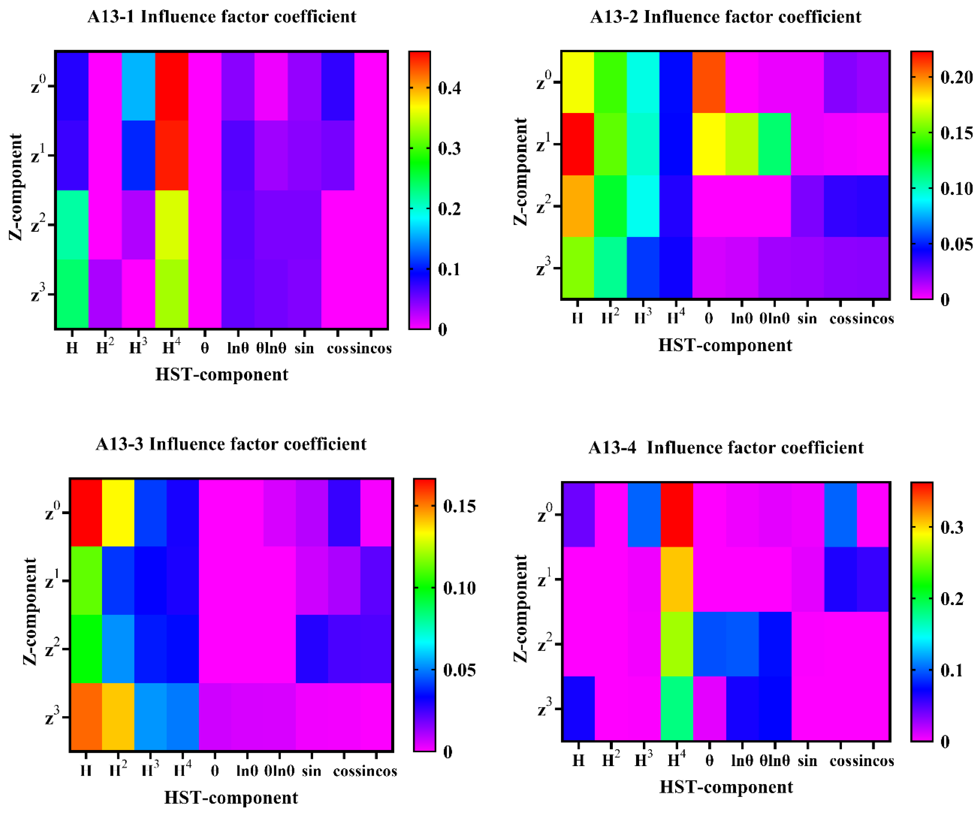
2.4. Optimal Factor Selection Principle Based on LASSO Regression

The complexity of the prediction model is directly related to the number of input variables. As the number of variables entering the model increases, the model becomes more complex. To combat this problem, the LASSO algorithm takes the ingenious approach of constructing a penalty function to refine the model. By increasing the coefficient of the penalty function, LASSO makes the coefficient of some variables in the model gradually shrink to 0. In this way, the LASSO [26] algorithm can quickly select important variables, thus reducing the complexity of the model and effectively avoiding the phenomenon of overfitting in the model. Its optimization objective function is:

$$\begin{array}{c}{\widehat{\beta }}^{lasso}=\arg \min \left\{{\displaystyle \sum _{i=1}^N}{\left(y_i-{\beta }_0-{\displaystyle \sum _{j=1}^p}{x}_{ij}{\beta }_j\right)}^2\right\}\\ \mathrm{s}.\mathrm{t}.\parallel \beta {\parallel }_1={\displaystyle \sum _{j=1}^p}\left|{\beta }_j\right|\le t\end{array}$$

(17)

where $y_i$ is the dependent variable; ${\beta }_0$ is the regression coefficient; $x_{ij}$ is an independent variable; ${\beta }_j$ is the regression coefficient; $N$ is the number of regression groups; and $P$ is the number of independent variables.

By substituting the constraints into the above formula, we can get:

$$\widehat{\beta }=\arg \min \left\{\sum _{i=1}^N{\left(y_i-{\beta }_0-\sum _{j=1}^p{x}_{ij}{\beta }_j\right)}^2+\sum _{j=1}^p\left|{\beta }_j\right|\right\}$$

(18)

where $\lambda \ge 0$ is the penalty function coefficient.

The LASSO algorithm will automatically obtain an optimal value $\lambda$. In the process of model iterative training, the regression coefficients of some influence factors will gradually shrink and tend to zero. At this time, these variables tending to zero can be eliminated.

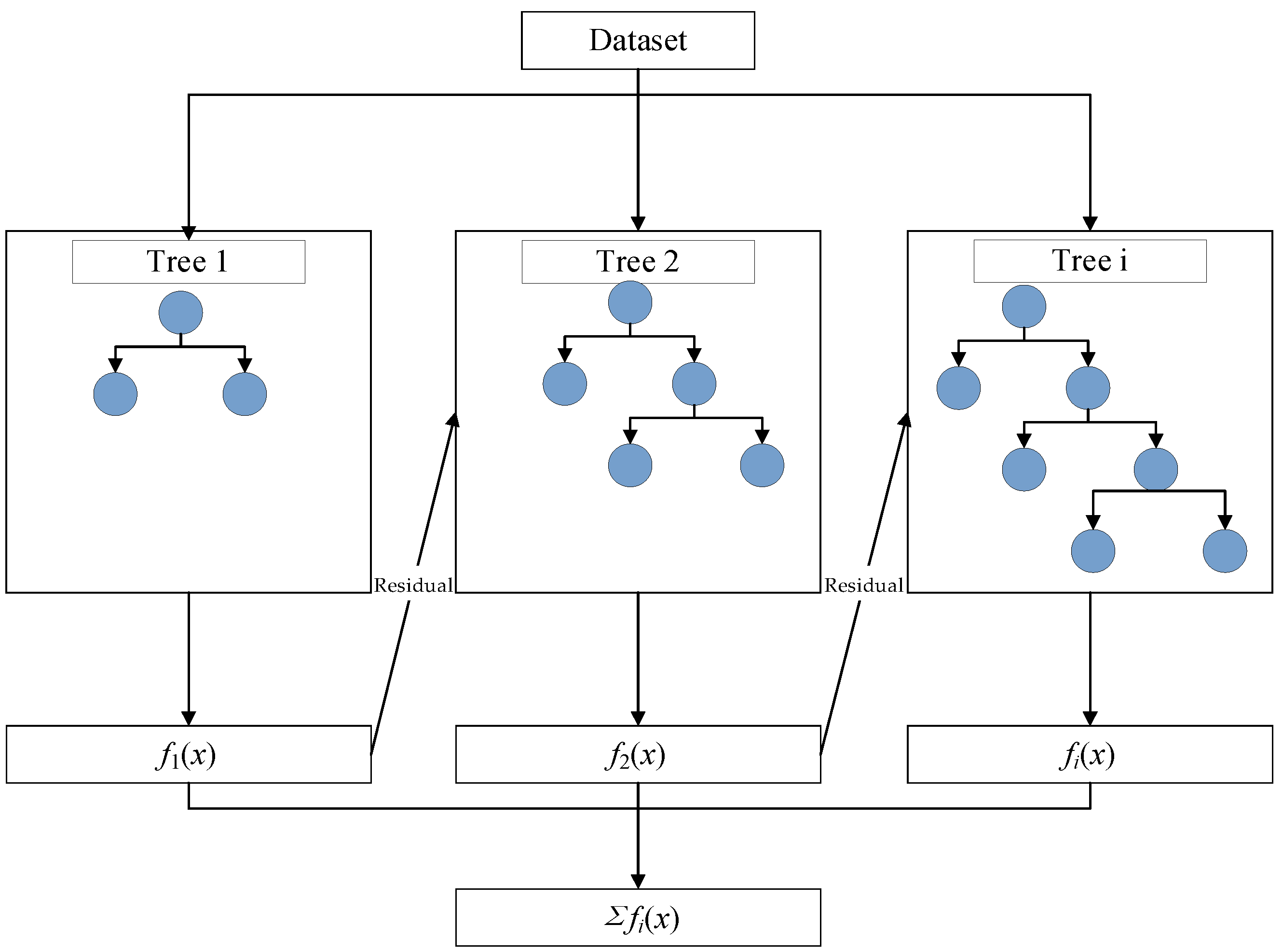
2.5. XGBoost Algorithm Principle

XGBoost [27,28] is an extension of the GBM algorithm and a prediction model with both linear regression and regression tree characteristics. In the XGBoost algorithm, there are multiple tree structures, each of which contains multiple branches (decision trees). The generation of each decision tree is adjusted according to the prediction results of the previous decision tree. Taking into account the prediction bias of the previous decision tree, we can gradually correct the prediction results. Each decision tree is generated by taking into account the entire dataset to optimize the model on the largest scale (Figure 6).

XGBoost corrects residuals from the last prediction by constantly adding new decision trees to the model and avoids overfitting problems through introducing regularization parameters [29]. Finally, XGBoost adds the weighted sum of the predictions from multiple decision trees to obtain the final prediction result. When building the dam deformation prediction model, the XGBoost algorithm can make use of the dam displacement data and constantly introduce temperature, aging, water pressure, and other factors into the model, as well as comprehensively consider and evaluate the influence of these factors on the dam deformation by approximating the actual displacement value. With XGBoost’s optimization and weighted summation method, the deformation of the dam can be predicted more accurately, and the importance of different factors can be assessed. This makes XGBoost a powerful and flexible tool for dam deformation prediction.

$${\widehat{y}}_k={\displaystyle \sum _{i=1}^k{G}_i\left(x_i\right)}=G_{k-1}\left(x_i\right)+f_k\left(x_i\right)$$

(19)

Here, $k$ is the number of predicted rounds; ${\widehat{y}}_k$ is the predicted value of dam displacement in the $k$ th round; and $f_k\left(x_i\right)$ is a tree function of temperature, aging, and water pressure factors. The objective function of the XGBoost algorithm is as follows:

$$\phi ={\displaystyle \sum _{i=1}^{k}l\left[y_i,f_{t-1}\left(x_i\right)+f_t\left(x_i\right)\right]}+\Omega \left(f_t\right)$$

(20)

where $k$ is the number of predicted rounds; and $l$ is the loss function of the relevant $y_i$, $f_t\left(x_i\right)$, where $y_i$ is the actual value of deformation displacement. The model training is completed when the objective function is found to be at the minimum through iteration.

2.6. Dam Deformation Prediction Model

The construction process and input of the dam deformation prediction model are as follows:

(1)

EEMD decomposition is performed on the measured value of dam displacement monitoring to obtain several $IMF$ components—$I=\left(IM{F}_1,IM{F}_2,\dots ,IM{F}_k\right)$—using the Pearson correlation coefficient between $IM{F}_i(i=1,2,\dots ,k)$ and $y_n$. When $C_i(i=1,2,\dots ,k)$ is less than the threshold, it is considered to be a noise-containing component. The noise-containing component is denoised by using the wavelet packet, and the noise reduction effect is verified by the comparison of curve smoothness and noise reduction error, and then the measured value of a certain measurement point after noise reduction is reconstructed.

(2)

Based on environmental variables such as the installation elevation and upstream water level of a measuring point, three types of factors, such as water pressure, temperature, and aging, of the measuring point were calculated as input variables, and the measured displacement history data of the measuring point after noise reduction was used as output variables to establish the LASSO model. The optimal factor was selected using the LASSO feature.

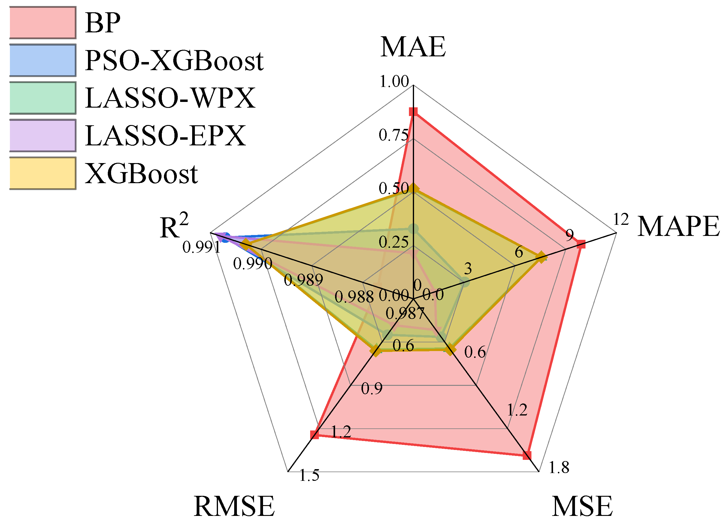
(3)

The root mean square error (RMSE), mean absolute percentage error (MAPE), coefficient of determination (R²), mean square error (MSE), and mean absolute error (MAE) were used to comprehensively compare the prediction models.

$$\left\{\begin{array}{l}{E}_{\mathrm{RMSE}}=\sqrt{{\displaystyle \frac{1}{N}}{\displaystyle \sum _{i=1}^N{\left(y(i)-y{(i)}^{\text{'}}\right)}^2}}\hfill \\ E_{\mathrm{MSE}}={\displaystyle \frac{1}{N}}{\displaystyle \sum _{i=1}^N{\left(y(i)-y{(i)}^{\text{'}}\right)}^2}\hfill \\ R^2=1-{\displaystyle \frac{{\displaystyle \sum _{i=1}^N{\left(y(i)-y{(i)}^{\text{'}}\right)}^2}}{{\displaystyle \sum _{i=1}^N{\left(\overline{y(i)}-y{(i)}^{\text{'}}\right)}^2}}}\hfill \\ E_{\mathrm{MAPE}}={\displaystyle \frac{1}{N}}{\displaystyle \sum _{i=1}^N\frac{y(i)-y{(i)}^{\text{'}}}{y(i)}}\times 100\%\hfill \end{array}\right.$$

(21)

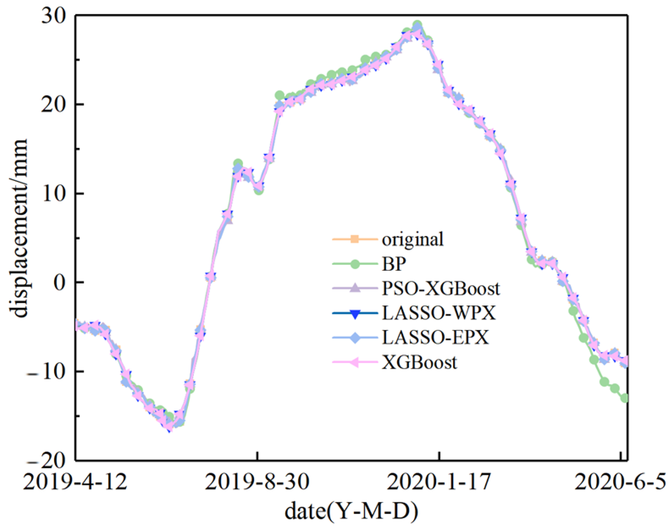
In the above formula, $y(i)$ is the $i$th measured displacement value; $y{(i)}^{\text{'}}$ is the $i$th predicted displacement value; and $N$ indicates the data length.

As important statistical indicators, the RMSE and MAE are used to evaluate the performance of predictive models. The RMSE is the root of the mean value of the squared error, and the smaller the value, the better the prediction effect is. However, since the expression equation contains the square error, it is more sensitive to the poorly predicted points and can be used as an indicator to measure the local prediction ability of the model. The MAE assesses the closeness between the predicted and measured values, and it reflects the overall forecasting error state. It is insensitive to outliers and can, therefore, be used to assess the overall prediction accuracy of the model.

The correlation coefficient R², also known as the Pearson correlation coefficient, reflects the degree of correlation between two variables, namely the correlation between the predicted value and the actual value. The closer the R² value is close to 1, the stronger the correlation between the two variables is and the better the model performance is (Figure 7).

3. Case Analysis

Based on the method described above, we chose a concrete engineering example to verify the effectiveness of the proposed method. The project is a double-curved arch dam with a total storage capacity of 7.76 billion cubic meters, being a 300 m high dam with a maximum dam height of 305 m, located along the lower Yalong River. In operation, the reservoir has functioned in many ways for power generation, flood control, and reservoir dispatching. We selected data from 2015 to 2021, with a total of 1902 sets related to the factors of upstream water level, ambient temperature, calculation aging, temperature, water pressure, and other factors for analysis and calculation. There are more than 30 positive and negative vertical displacement measurement points from the dam top to the dam foundation, and the highest section of the dam height is selected. The original data are divided into training set and test set, and the ratio of the training set to the test set is 8:2. Four measuring points from A13-1 to A13-4 were selected to establish a spatial correlation model for verification (Figure 8).

3.1. Sequence Decomposition

Using the methods in Section 2.3, in the EEMD algorithm, the parameters are set to $\alpha =0.15$ and $n=100$. And the correlation coefficient between the modal component and the measured value after the decomposition of the measured displacement at each measuring point is calculated as shown below (Figure 9 and

Table 1. Phase relation table.

Measuring Point	IMF Number	${\mathit{C}}_1$	${\mathit{C}}_2$	${\mathit{C}}_3$	${\mathit{C}}_4$	${\mathit{C}}_5$	${\mathit{C}}_6$	${\mathit{C}}_7$	${\mathit{C}}_8$	${\mathit{C}}_9$	${\mathit{C}}_{10}$	${\mathit{C}}_{11}$	${\mathit{C}}_{12}$
A13-1	11	0.012	0.040	0.000	0.061	0.087	0.129	0.211	0.863	0.768	0.225	0.173
A13-2	11	−0.019	−0.035	−0.007	0.057	0.049	0.116	0.227	0.821	0.805	0.208	0.202
A13-3	11	−0.009	−0.029	0.007	0.033	0.077	0.124	0.200	0.790	0.840	0.271	0.190
A13-4	12	0.002	0.012	0.016	0.022	0.033	0.110	0.157	0.757	0.827	0.163	0.269	0.096

):

It can be seen from the Table 1 that the correlation coefficients of A13-1 to A13-4 are all below 0.25, which can be judged to be high-frequency signals, and then, the wavelet method is used for noise reduction. The comparison between the measured value after noise reduction and the measured value before noise reduction is shown in Figure 10 and Figure 11.

The same calculation was carried out for A13-2 to A13-4, and the result was represented by a heat map. $H$, $H^2$, $H^3$, $H^4$ are water level to the power of one, two, three, and four, respectively. $zH$, $z{H}^2$, $z{H}^3$, $z{H}^4$ are are the first power, second power, third power, and fourth power of the water level after the change. The greater the influence coefficient of the warmer colored region, the greater the importance of the corresponding factor (Figure 12 and

Table 2. Regression coefficient table of influence factors.

Measuring Point	${\mathit{\delta }}_{\mathit{W}}$ Hydraulic Pressure
A13-1	$H$		$H^2$			$H^3$		$H^4$			$zH$		$z{H}^2$		$z{H}^3$		$z{H}^4$
	0.108		0.000			0.187		0.490			0.101		0.000		0.135		0.470
	$z^{2}H$		$z^2{H}^2$			$z^2{H}^3$		$z^2{H}^4$			$z^{3}H$		$z^3{H}^2$		$z^3{H}^3$		$z^3{H}^4$
	0.217		0.000			0.028		0.354			0.237		0.030		0.000		0.335
Measuring Point	${\delta }_{\theta }$ Aging Factor									${\delta }_T$ Temperature Factor
A13-1	$\theta$	$\ln \theta$		$\theta \ln \theta$	$\theta z$		$\theta z^2$		$\theta z^3$	$\sin$		$\cos$	$\sin \cos$	$z\sin$		$z^2\sin$		$z^3\sin$
	0.000	0.072		0.016	0.000		0.000		0.000	0.048		0.084	0.000	0.032		0.034		0.036
	$z\ln \theta$	$z^2\ln \theta$		$z^3\ln \theta$	$z\theta \ln \theta$		$z^2\theta \ln \theta$		$z^3\theta \ln \theta$	$z\cos$		$z^2\cos$	$z^3\cos$	$z\sin \cos$		$z^2\sin \cos$		$z^3\sin \cos$
	0.042	0.050		0.052	0.032		0.043		0.080	0.045		0.000	0.000	0.000		0.000		0.000

):

As can be seen from the Table 1 and Table 2 and Figure 12, the main factors affecting the displacement and deformation data are concentrated on the water pressure component, and the aging component is occasionally seen. Although the temperature and aging factor are weaker than the water pressure, the temperature component still needs to be considered.

3.2. Comparison of Prediction Results

In order to verify the effectiveness of the dam temporal and spatial prediction model based on the Z-component, this model (EEMD-LASSO-PSO-XGBoost, referred to as LASSO-EPX, the same below) was compared with PSO-XGBoost, LASSO-WPX, and XGBoost, taking the measuring point A13-1 as an example. This model was compared with BP to verify the excellent performance of XGBoost under multiple combinatorial optimization algorithms.

As shown in the Figure 13, the LASSO-EPX and LASSO-WPX models fit the original data well, but the LASSO-WPX model fits poorly in the latter half of the curve. The fit degree of the BP neural network, C-X, and PSO-XGBoost algorithms is worse than that of LASSO-EPX.

As shown in the Table 1 and Table 2, LASSO-EPX maintains the maximum R² while maintaining the minimum value for the MAE, MAPE, MSE, and RMSE. According to the evaluation index of the prediction model, the LASSO-EPX algorithm proposed in this paper has a higher accuracy than other models (Figure 13).

As can be seen from the

Table 3. Prediction model evaluation index table.

Model	BP	PSO-XGBoost	LASSO-WPX	LASSO-EPX	XGBoost
MAE	0.8736	0.3268	0.5105	0.2126	0.5148
MAPE	9.9174	3.0211	7.5618	1.2723	7.5704
MSE	1.6333	0.3957	0.5177	0.3270	0.5277
RMSE	1.3447	0.6502	0.7527	0.5829	0.7604
R2	0.9877	0.9907	0.9903	0.9908	0.9903

and Figure 13, the main influencing factors affecting the displacement and deformation data are concentrated on the water pressure component, and the aging component is occasionally seen. Although the temperature and aging factor are smaller than the water pressure, the temperature component still needs to be considered. Each model evaluation index was listed in Figure 14.

4. Conclusions

In this paper, EEMD, wavelet noise reduction, the particle swarm optimization algorithm, and XGBoost and LASSO feature selection of a multi-point prediction model considering spatial correlation are comprehensively used. The main conclusions are as follows:

(1)

The ways of considering the spatial correlation of measurement points, selecting an algorithm according to features, and focusing on the key environmental factors can effectively help reflect the main factors affecting the effect size.

(2)

In the EEMD–wavelet denoising model, the sharp points and gross errors of the original data are eliminated on the premise of reducing the calculation errors and retaining the features of the original data, and the accuracy and precision of the prediction model are improved.

(3)

By comparing the accuracies of the prediction models, the MAE, MAPE, MSE, RMSE, and R² of the LASSO-EPX model are superior to other models mentioned in this paper, which is significantly improved after a comparison with the BP neural network.