Action-Oriented Deep Reinforcement Learning Method for Precast Concrete Component Production Scheduling

Abstract

In the production scheduling of precast concrete components, decision makers often face the challenges of complex decision making and incomplete decision information due to the lack of real-time and comprehensive insights into subsequent production stages after the initial scheduling phase. To address these, this study proposes an action-oriented reinforcement learning (AO-DRL) method aimed at minimizing the maximum completion time. Firstly, the set of unscheduled components is defined as the action space, eliminating the need for designing extensive dispatching rules. Secondly, dynamic processing features that evolve with the production environment are extracted as action representations, providing the agent with comprehensive decision-making information. Thirdly, the Double Deep Q-Network (DDQN) algorithm is employed to train the AO-DRL model, enabling it to capture the dynamic relationship between the production environment and the unscheduled components for effective scheduling decisions. Finally, the proposed approach is validated using randomly generated samples across various problem scales. The experimental results demonstrate that AO-DRL outperforms traditional rule-based methods and heuristic algorithms while exhibiting strong generalization capabilities.

1. Introduction

The construction industry is currently facing a number of challenges related to environmental protection, economic efficiency, and engineering quality on a global scale. In light of these circumstances, prefabricated construction, as a novel construction mode characterized by intensive industrialization, is progressively emerging as a pivotal avenue for the industry’s transformation and modernization. With its efficient production process, superior construction quality and substantial environmental benefits, prefabricated construction has not only gained a foothold in the housing and infrastructure construction of developed countries, but has also garnered extensive market acceptance and policy endorsement in developing countries.

The core of prefabricated construction lies in the processes of production and construction. Precast concrete components (PCCs) are typically prefabricated in factories and subsequently transported to construction sites for assembly. This process entails numerous interrelated stages, including production, transportation, and assembly. Among them, production is the core stage affecting the progress and cost of prefabricated construction. Its task is to optimize the production sequencing of PCCs and the allocation of workstations within the cycle time. This problem is essentially a type of flowshop scheduling problem (FSP), proved as an NP-hard problem [1]. It is challenging to obtain an exact solution within the allowable time. Especially when facing unexpected factors (such as natural disasters, production interruptions, or schedule changes), the flexible scheduling and optimization of production plans become particularly crucial, as they directly impact the overall quality of construction, the efficiency of construction, and the reliability of project delivery [2,3].

To achieve production scheduling optimization methods aimed at enhancing production efficiency and reducing costs, researchers have proposed various approaches, mainly including heuristic dispatching rules and metaheuristic algorithms. The heuristic dispatching rule refers to any empirical rule for prioritizing the processing of PCC, such as the rules of shortest processing time first (SPT) and earliest delivery date first (EDD). Due to its low computational complexity and fast processing efficiency, the heuristic dispatching rule can rapidly generate a satisfactory solution in the simple production-scheduling scenario. However, as the scenario becomes more complex, this approach cannot guarantee the optimal performance of the solution.

Metaheuristic algorithms, such as genetic algorithms (GAs) [4], particle swarm optimization (PSO) [5] and grey wolf optimizers (GWOs) [6], find optimal or near-optimal solutions to a constrained problem within a reasonable time by employing a combination of global and local search strategies. Although these algorithms and their variants have been very popular in FSP, there are still some limitations. Firstly, in the event of a change to the production environment, such as the arrival of a new order or the initiation or cessation of equipment operation, the input and output representation and the parameters of the algorithm need to be re-modified. Secondly, each calculation process of the algorithm is executed independently. The experience and knowledge gained in previous iterations cannot be utilized, resulting in an inefficient use of computing resources. Thirdly, as the problem size increases, the computational complexity of the algorithm exhibits nonlinear growth, leading to a significant increase in solution time.

For discrete combinations of complex systems, the reinforcement learning (RL) approach has attracted widespread attention from scholars with its advantages in solving sequential decision-making problems [7,8]. RL is based on Markov decision processes. The agent gradually improves its decision-making strategy through continuous interaction with the environment, driven by the expected return, with the objective of maximizing the cumulative long-term reward [9]. The well-designed RL can be applied to problems of different scales, and can be used to make real-time decisions by leveraging decision-making experience learned from historical cases [10]. Despite the great potential of RL in production-scheduling problems, there remain some limitations in the existing research. On the one hand, the action space is designed based on heuristic dispatching rules, which may limit the decision-making space of the agent. In some cases, the rule-based action space is unable to fully cover the dispatching needs of all components, thus forming blind spots in the decision-making process. On the other hand, when faced with incoherence or delay in environmental feedback information, the rule-oriented deep reinforcement learning approach (RO-DRL) encounters difficulties in establishing an accurate environment–rule mapping relationship, which in turn affects the quality of decision-making.

Therefore, this study proposes an action-oriented reinforcement learning approach (AO-DRL) for PCC production scheduling. The main contributions of this study include:

A PCC production-scheduling model that is consistent with actual environment has been constructed, taking into account factors such as flow constraints and transfer times between workstations, which improves the practicality and accuracy of the model.

A set of global state features based on the perspective of the workstation has been designed.

A set of state features of the action space is proposed for establishing the interaction between the action and the environment from a microscopic perspective.

A novel scheduling decision-making strategy is proposed, which employs a Double Deep Q-Network (DDQN) to calculate directly value between action and environment.

The remainder of this paper is organized as follows. Section 2 gives a review of production-scheduling methods. Section 3 establishes a mathematical model of PCC production scheduling. The implementation details of AO-DRL are provided in Section 4. The results of numerical experiments are given in Section 5. Section 6 presents a comprehensive analysis. Finally, conclusions are drawn in Section 7.

2. Literature Review

A reasonable production plan for PCC is crucial for construction progress management and cost control in prefabricated construction. The production scheduling problem of PCC can be defined as a combinatorial optimization problem, which can be classified as FSP [11]. Since Johnson first revealed the flowshop scheduling problem in 1954, researchers have conducted extensive research and developed rich models and algorithms. These methods can be classified into two principal categories, namely (1) an exact algorithm and (2) an approximate algorithm.

Precision algorithm, including branch and bound, mixed integer programming, and dynamic programming, can provide an exact solution to the problem due to its excellent global optimization capabilities. These algorithms are particularly suitable for solving FSP in single-machine production or small-scale production scenarios [12]. However, since the 1970s, with the significant increase in productivity and the expansion of production scale, the complexity and scale of FSP have also increased significantly. This has made it difficult for traditional exact algorithms to obtain the high-quality solution within an acceptable time. Consequently, the focus of research on FSP has gradually shifted towards approximate algorithms, with the aim of achieving a balance between solution efficiency and solution accuracy.

An approximate algorithm mainly includes the heuristic dispatching rule approach, the metaheuristic algorithm, and the gradually emerging machine learning approach.

The heuristic dispatching rule approach evaluates the priority of jobs by a series of priority rules, and then sorts them in order of their evaluated priorities to form a complete dispatching solution. Panwalker et al. [13] summarised 113 different dispatching rules, including simple dispatching rules, combined dispatching rules, heuristic dispatching rules, etc. Calleja and Pastor [14] proposed a dispatching-rule-based algorithm and introduced a mechanism for manually adjusting the priority rule weights in order to solve the problem of flexible workshop scheduling with transfer batches. Liu et al. [15] designed a heuristic algorithm comprising eight combined priority rules to optimise the scheduling of multiple mixers in a concrete plant. The heuristic dispatching rule approach is still employed in practical production due to its straightforward implementation, ease of operation, and rapid calculation. However, this approach is constrained by its inability to achieve global optimality and it is difficult to estimate the gap between the outcome and the optimal solution, leaving much room for improvement.

The metaheuristic algorithm combines a stochastic algorithm and a local search strategy. The algorithm initially generates some initial solutions, and then iteratively modifies them with heuristic strategies, so as to explore the larger solution space and effectively find a high-quality solution within an acceptable time. Wang et al. [16] proposed a genetic algorithm-based PCC production-scheduling model that considers the storage and transportation of components. Dan et al. [17] proposes an optimization model for the production scheduling of precast components from the perspective of process constraints, including process connection and blocking, and it is solved by GA. Qin et al. [18] considered the resource constraints in the production process and constructed a mathematical model for PCC production scheduling with the objective of Maxspan and cost. The model was solved using an improved multi-objective hybrid genetic algorithm. Since the single heuristic algorithm is constrained in global or local search capabilities, it can lead to local optimization. Therefore, the research on the combination of various heuristic algorithms has flourished. Xiong et al. [19] proposed a hybrid intelligent optimization algorithm based on adaptive large neighbourhood search for solving the optimization problem of distributed PCC production scheduling. The method combines heuristic rules for dynamic neighbourhood extraction with a tabu search algorithm to enhance the quality of the initial solution. Furthermore, multiple neighbourhood structures were introduced to avoid the premature convergence of the algorithm into a local optimum. Xiong et al. [20] established an integrated model for the optimization of PCC production scheduling and worker allocation, with the objective of minimizing worker costs and delay penalties. They proposed an efficient hybrid genetic–iterative greedy alternating search algorithm to solve it. Compared with a single intelligent optimization algorithm, this algorithm has better performance in terms of efficiency, stability and convergence.

As the means of production continue to develop, FSP has given rise to a variety of complex variants. Some pioneering research focuses on the dynamic production scheduling of PCC, exploring rescheduling strategies under operational uncertainty or demand fluctuations [21,22]. Kim et al. [23] incorporated the inherent uncertainty of construction progress into the production scheduling of PCC, and proposed a dynamic scheduling model that can respond to changes in due dates in real time and minimize delays. Similarly, Du et al. [24] studied dynamic scheduling under production delays caused by internal factors in the precast factory and changes in demand caused by external factors. Moreover, most scholars have devoted to flexible FSP(FFSP). FFSP represents a significant advance in production efficiency compared to traditional FSP, but it requires simultaneous consideration of the scheduling of jobs, machines, and workstations. Jiang et al. [25] designed a discrete cat-swarm optimization algorithm to solve FJSP with delivery time. An et al. [26] established an integrated optimization model for production planning and scheduling in a flexible workshop and proposed a decomposition algorithm based on Lagrangian relaxation, which decomposes the integrated problem into production planning subproblems and scheduling subproblems for separate solution. Zhang et al. [27] proposed an improved multi-population genetic algorithm for the multi-objective optimization of flexible workshop scheduling problems, with a particular focus on the shortest processing time and the balanced utilization of machines. Although metaheuristic algorithms are widely used in practical production due to their flexibility and wide applicability, they have problems of high computational intensity and difficulty in tuning [28].

In recent years, reinforcement learning has attracted considerable attention due to its distinctive goal-oriented unsupervised learning capacity. However, when faced with massive high-dimensional data, RL reveals its weaknesses of low sampling efficiency and state-dimension disaster. In response, researchers have combined deep learning with reinforcement learning to form a DPL algorithm, which organically combines deep learning with perceptual capabilities and reinforcement learning with decision-making capabilities [8]. DRL does not rely on environmental models or historical prior knowledge. It needs to interact with the environment to learn current experience to train the neural network. This not only solves the difficulty of the deep learning training process, which requires a lot of high-quality prior knowledge, but also overcomes the ‘explosion of dimensions’ problem [28]. DRL has been shown to have a strong learning ability and optimal decision-making ability in complex scenarios such as Atari [29] and AlphaGo Zero [30]. In recent years, DRL has been applied to the field of production scheduling and has made certain research progress [31].

DRL approaches to solving FSP can be classified into two main categories: indirect and direct approach. The indirect approach typically entails the utilization of reinforcement learning to optimize the parameters of metaheuristic algorithms to improve their ability to solve FSP [32]. Emary et al. [33] used RL combined with a neural network to improve the global optimization ability of GWO.

The direct approach focuses on creating an end-to-end learning system that can directly map from state to action, directly making scheduling decisions. This approach can quickly generate the scheduling solution and is suitable for handling large-scale scheduling problems. Chen et al. [34] proposed an an Interactive Operation Agent (IOA) scheduling model framework based on DRL approaches, which aims to solve the frequent re-scheduling problem caused by machine failures or production disturbances. In this framework, the processing steps in the workshop are constructed as independent process agents, and the scheduling decisions are optimized through feature interaction, which demonstrates robust and generalisable capabilities. Luo et al. [35] employs a Deep Q-Network (DQN) to address dynamic and flexible workshop scheduling problem with new job insertions. Du [36] designed an architecture consisting of three coordinated DDQN networks for the distributed flexible scheduling of PCC production. Chang et al. [37] employed a Double Deep Q-Network as an agent to address the dynamic job shop scheduling problem (JSP) with random task arrivals, with the objective of minimizing delays. Wang et al. [38] conducted further research into the dynamic multi-objective flexible JSP problem.

However, the above DRL studies on production scheduling predominantly employ general or custom dispatching rules to define the action space. While this approach integrates prior knowledge, it heavily relies on expert input, thereby limiting the agent’s decision-making scope to the boundaries set by these predefined rules. Moreover, when the agent receives indirect environmental feedback after executing actions based on these rules, it struggles to establish a clear mapping between the environmental state and the dispatching rules. This limitation adversely affects both the learning efficiency and the quality of decision making.

In response to these challenges, this study introduces an action-oriented deep reinforcement learning (AO-DRL) approach. Diverging from methods that depend extensively on predefined rules, AO-DRL defines the action space in terms of unscheduled components. It selects actions by directly evaluating the long-term performance of these components within the current environmental context. This innovative approach not only diminishes the reliance on expert knowledge but also enhances the agent’s adaptability to dynamic environments.

3. Problem Formulation

3.1. Problem Description

Production-scheduling problem description: The production line comprises M processing stations for producing N components. Each component is subjected to six processes, as detailed in Figure 1. Each process can only be completed at its designated station, with varying processing time across different components. The primary objective is to determine the optimal production sequence of these components to achieve the shortest completion time. For each component, appropriate processing stations for each process of every component should be assigned, as well as the precise start and completion times for each process.

Constraints in precast concrete component production scheduling are as follows:

• Station Resource Constraints: Excluding the station corresponding to p5, each processing station is constrained to handle a single component at any given time.
• Process Typology Constraints: Processes are bifurcated into interruptible (p1, p2, p3, p6) and non-interruptible (p4, p5) categories. Interruptible processes allow the incomplete operations to be carried over to the next day, whereas non-interruptible processes must be completed continuously once initiated. Furthermore, overtime may be scheduled for p4 when necessary.
• Process Sequentiality Constraints: The concrete-pouring (p4) and steam-curing (p5) operations must be continuous with no idle time.
• Production Sequencing Constraints: Due to the absence of buffer zones within the production line, component processing follows the first-in-first-out principle.

The definitions of relevant symbols used in this study are presented in

Table 1. Notations used for problem formulation.

Notation	Description
$\zeta$	precast concrete component set, $\zeta =\{1,\dots ,N\}$, N is total number of precast concrete components
P	process set, $P=\{p_1,p_2,p_3,p_4,p_5,p_6\}$
$\phi$	workstation set, $\phi =\{1,\dots ,M\}$, M is total number of workstations
$\phi \left(p\right)$	the set of workstations corresponding to process p
$i,j$	Index of precast concrete component
p	Index of process
m	Index of workstation
$\overleftarrow{m}$	Index of workstation of the previous process
$\overrightarrow{m}$	Index of workstation of the subsequent process
$H_w$	Normal working hours per day
$H_o$	Allowed overtime per day
$t_o$	Transfer time between neighbouring stations
$t_{jp}$	Processing time for process p of precast concrete component $\phi \left(p\right)$
$S_{jmp}$	Start time of process p at workstation m for precast concrete component j
$C_{jmp}^{\prime }$	Estimated completion time of process p at workstation m for precast concrete component j
$C_{jmp}$	Actual completion time of process p at workstation m for precast concrete component j
$D_{jmp}$	Actual leave time of precast concrete component j after process p is completed at workstation m
$x_{jmp}$	If precast concrete component j is assigned to workstation m for process p, then it is 1; otherwise, it is 0.
$Y_{ijm}$	If precast concrete component i and j enter the same workstation m sequentially, then it is 1; otherwise, it is 0.
${\epsilon }_{jmp}$	If precast concrete component j is first processed on workstation m for process p, then it is 1; otherwise, it is 0.

.

3.2. Optimization Scheduling Model for Precast Concrete Component Production

3.2.1. Optimization Objective

The optimization goal is to minimize the maximum completion time (Maxspan) of precast concrete components.

$$minC=max\left(D_{jm6}\right),\forall j\in \zeta ,m\in \phi \left(6\right)$$

(1)

3.2.2. Constraint

$$\sum _{m\in \phi \left(p\right)}{x}_{jmp}=1,\forall j\in \zeta ,\forall p\in \tau$$

(2)

$$\sum _{m\in \phi \left(p\right)}\sum _{p\in \tau }{x}_{jmp}=6,\forall j\in \zeta$$

(3)

$$S_{jm1}=0,if{\epsilon }_{jm1}=1,m\in \phi \left(1\right)$$

(4)

$$\begin{array}{c}{S}_{jm1}\ge D_{im1}-M(1-Y_{ijm}),if{\epsilon }_{jm1}=0,\forall j\in \zeta ,m\in \phi \left(1\right)\hfill \end{array}$$

(5)

$$\begin{array}{c}{S}_{jm1}\le D_{im1}+M(1-Y_{ijm}),if{\epsilon }_{jm1}=0,\forall j\in \zeta ,m\in \phi \left(1\right)\hfill \end{array}$$

(6)

$$\begin{array}{c}{S}_{jmp}=D_{j\overleftarrow{m}(p-1)}+DIJL(\overleftarrow{m},m)\ast t_0,\forall j\in \zeta ,p\in (2,3,4,5,6),m\in \phi \left(p\right),\overleftarrow{m}\in \phi (p-1)\hfill \end{array}$$

(7)

$$\begin{array}{c}{C}_{jmp}^{\prime }=S_{jmp}+t_{jp},\forall j\in \zeta ,\forall p\in \tau \hfill \end{array}$$

(8)

$$\begin{array}{c}{C}_{jmp}\ge C_{jmp}^{\prime }-M(1-x_{imp}),if{C}_{jmp}^{\prime }\le ⌊{\displaystyle \frac{C_{jmp}^{\prime }}{24}}⌋\ast 24+H_w,\forall j\in \zeta ,\forall p\in \tau ,m\in \phi \left(p\right)\hfill \end{array}$$

(9)

$$\begin{array}{c}{C}_{jmp}\le C_{jmp}^{\prime }+M(1-x_{imp}),if{C}_{jmp}^{\prime }\le ⌊{\displaystyle \frac{C_{jmp}^{\prime }}{24}}⌋\ast 24+H_w,\forall j\in \zeta ,\forall p\in \tau ,m\in \phi \left(p\right)\hfill \end{array}$$

(10)

$$\begin{array}{c}{C}_{jmp}\ge C_{jmp}^{\prime }+24-H_w-M(1-x_{imp}),if{C}_{jmp}^{\prime }\ge ⌊{\displaystyle \frac{C_{jmp}^{\prime }}{24}}⌋\ast 24+H_w,\forall j\in \zeta ,p\in (1,2,3,6),m\in \phi \left(p\right)\hfill \end{array}$$

(11)

$$\begin{array}{c}{C}_{jmp}\le C_{jmp}^{\prime }+24-H_w+M(1-x_{imp}),if{C}_{jmp}^{\prime }\ge ⌊{\displaystyle \frac{C_{jmp}^{\prime }}{24}}⌋\ast 24+H_w,\forall j\in \zeta ,p\in (1,2,3,6),m\in \phi \left(p\right)\hfill \end{array}$$

(12)

$$\begin{array}{c}{C}_{jm5}\ge \left[{\displaystyle \frac{C_{jm5}^{\prime }}{24}}\right]\ast 24+24-M(1-x_{im5}),if{C}_{jm5}^{\prime }\ge ⌊{\displaystyle \frac{C_{jm5}^{\prime }}{24}}⌋\ast 24+H_w,\forall j\in \zeta ,m\in \phi \left(5\right)\hfill \end{array}$$

(13)

$$\begin{array}{c}{C}_{jm5}\le ⌊{\displaystyle \frac{C_{jm5}^{\prime }}{24}}⌋\ast 24+24+M(1-x_{im5}),if{C}_{jm5}^{\prime }\ge ⌊{\displaystyle \frac{C_{jm5}^{\prime }}{24}}⌋\ast 24+H_w,\forall j\in \zeta ,m\in \phi \left(5\right)\hfill \end{array}$$

(14)

$$\begin{array}{c}{D}_{jm4}=C_{jm4}=C_{jm4}^{\prime },\forall j\in \zeta ,m\in \phi \left(4\right)\hfill \end{array}$$

(15)

$$\begin{array}{c}{D}_{jmp}=max\{min\left(DIJT(m,\overrightarrow{m})\right),C_{jmp}\}\forall j\in \zeta ,p\in (1,2,5,6),m\in \phi \left(p\right),\overrightarrow{m}\in \phi (p+1)\hfill \end{array}$$

(16)

$$\begin{array}{c}{D}_{jm3}=max\{min\left(T_{\phi \left(5\right)}\right),min\left(DIJT(m,\overrightarrow{m})\right),C_{jm3}\},\hfill \\ if{C}_{jm3}+DIJL(m,\overrightarrow{m})\ast t_0+t_{j4}<=⌊{\displaystyle \frac{C_{jm3}}{24}}⌋\ast 24+H_w+H_o,\forall j\in \zeta ,m\in \phi \left(3\right),\overrightarrow{m}\in \phi \left(4\right)\hfill \end{array}$$

(17)

$$\begin{array}{c}{D}_{jm3}=max\{min\left(T_{\phi \left(5\right)}\right),min\left(DIJT(m,\overrightarrow{m})\right),\left[{\displaystyle \frac{C_{jm3}}{24}}\right]\ast 24+24\},\hfill \\ if{C}_{jm3}+DIJL(m,\overrightarrow{m})\ast t_0+t_{j4}>⌊{\displaystyle \frac{C_{jm3}}{24}}⌋\ast 24+H_w+H_o,\forall j\in \zeta ,m\in \phi \left(3\right),\overrightarrow{m}\in \phi \left(4\right)\hfill \end{array}$$

(18)

Equation (2) indicates that each process of PCC is assigned to only one workstation. Equation (3) indicates that all six processes of PCC are to be completed. Equation (4) initializes the start time of the first process of PCC. Equations (5) and (6) ensure the processing continuity between the previous and subsequent components in p1. Equation (7) denotes that the start time of the next process should be equal to its departure time plus the transfer time, representing the minimum number of transfers from workstation to workstation m calculated by the Dijkstra algorithm. Equation (8) calculates the estimated completion time of the process. Equations (9) and (10) indicate that if the process can be completed within normal working hours, the actual completion time is equal to the estimated completion time. $⌊A⌋$ denotes rounding down to A. Equations (11) and (12) denote the actual completion time of interruptible processes if they cannot be completed within normal working hours on the same day. Equations (13) and (14) guarantee that non-interruptible p5 can be completed outside of normal working hours. Equation (15) represents the process connection constraint between p4 and p5. Equation (16) calculates the estimated time when PCC leaves the workstation after completing p1, p2, p5, and p6, representing the minimum bottleneck time for a transfer path from m to be unobstructed. Equations (17) and (18) indicate the flow constraints between p3 and p4 of the same PCC. The former calculates the time at which PCC leaves the workstation of p3, given that p4 can be completed before the overtime; the latter calculates the time at which PCC leaves the workstation of p3, given that p4 cannot be completed before the overtime. Among these, $min\left(T_{\phi \left(5\right)}\right)$ indicates the earliest available time of curing chambers.

3.3. Simulation Algorithm of Precast Concrete Component Production

Unlike the manufacturing industry, where each process in the production line makes decisions independently, in PCC production, the production processes of a component are executed in a fixed sequence. Subsequent components cannot precede the preceding components in the processing order. Therefore, the core of the production decision making for PCC lies in determining the production sequence, while the process scheduling of PCC is automatically managed by the production simulation algorithm, as shown in Algorithm 1.

As p1 is usually carried out outside the production line, this study identifies the idle time of the workstation for p2 on the production line as the decision point. At this decision point, the algorithm selects a component from the unscheduled components set to enter the production line (Line 1–4). Following the first-in-first-out (FIFO) principle, an inverse allocation strategy is employed, where the earliest entering component is prioritized for assignment to the next process workstation. Subsequently, the algorithm schedules the processes for the remaining components in their order of entry (Line 5–11). In calculating the operating time for the next process of the component, the start and end times are adjusted based on the characteristic of the process (e.g., whether it can be interrupted) (Line 12–22). Once all components of $SC{S}_W$ have been scheduled, the algorithm updates the point time based on the earliest completion time among the components currently being processed, and updates the states of these components accordingly. When the workstation for p2 becomes available again, a new decision point is triggered, and the above steps are repeated until the all components are completed (Line 23–36).

Algorithm 1 The process-scheduling algorithm for PCC

Input: Unscheduled components set ($UCS$), scheduled components set ($SCS$) Output: Scheduled components processing times    1: while  $UCS\ne \varnothing$  do    2:       select component J from $UCS$ by action    3:       add component J to $SCS$    4:       remove component J from $UCS$    5:       calculate $SC{S}_W$, the subset of components waiting for process scheduling in $SCS$    6:       for component K in $SC{S}_W$ do    7:             if next process of component K is p1 then    8:                   calculate start time of next process for component K by Equations (5) and (6)    9:             else if condition then  10:                   calculate start time of next process for component K by Equation (7)  11:             end if  12:             calculate estimated finish time of next process of component K by Equation (8)  13:             if next process of component K is interruptible (p1, p2, p3, p6) and estimated finish time exceeds normal working hours then  14:                   calculate actual finish time by Equations (11) and (12)  15:             else if next process of component K is non-interruptible (p4) and estimated finish time exceeds overtime working hours then  16:                   schedule entire process for the next day  17:             else if next process of component K is non-interruptible (p5) and estimated finish time exceeds overtime working hours then  18:                   calculate actual finish time by Equations (13) and (14)  19:             else  20:                   actual finish time = estimated finish time  21:             end if  22:       end for  23:       calculate $SC{S}_P$, the set of components currently in processing in $SCS$  24:       if $SC{S}_P\ne \varnothing$ then  25:             select earliest finish time of current process of component L in $SC{S}_P$ as point time  26:             for component L in $SC{S}_P$ do  27:                   update status of current process of component L by comparing its actual finish time with point time  28:             end for  29:       end if  30:       if there is an available workstation for p2 and $UCS\ne \varnothing$ then  31:             exit loop  32:       end if  33:       if $SC{S}_P$ is empty and $UCS$ is empty then  34:             exit loop  35:       end if  36: end while

4. Double Deep Q-Network for Precast Concrete Component Production Scheduling

4.1. State Features

In the process of the agent interacting with the environment, state features are the basis for the agent to perceive the environment and make decisions accordingly. In terms of state features, this study quantitatively describes the global and local information of the production line, aiming to enhance the agent’s ability to perceive the subtle state differences.

At the global information level, six global state features are constructed to characterise the overall operation of the production line.

(1)

Average completion rate of all components

$$\begin{array}{c}{S}_1={\displaystyle \frac{{\sum }_{j\in \zeta }c{r}_j}{\left|\zeta \right|}}\hfill \end{array}$$

(19)

where $c{r}_j$ denotes completion rate of component j, and |*| denotes the cardinality of the set.

(2)

Percentage of completed components

$$\begin{array}{c}{S}_2={\displaystyle \frac{\left|CCS\right|}{\left|\zeta \right|}}\hfill \end{array}$$

(20)

where $CCS$ denotes the subset of completed components

(3)

The remaining normal working hours for the day

$$\begin{array}{c}{S}_3=H_o-\mathrm{mod}(dt,24)\hfill \end{array}$$

(21)

where $dt$ is the current decision point time, and $mod(a,b)$ indicates the modulo operation.

(4)

Percentage of scheduled components

$$\begin{array}{c}{S}_4={\displaystyle \frac{\left|SCS\right|}{\left|\zeta \right|}}\hfill \end{array}$$

(22)

where $SCS$ denotes a subset of scheduled components.

(5)

The day of the current decision point

$$\begin{array}{c}{S}_5=[dt,24]\hfill \end{array}$$

(23)

where $[a,b]$ denotes a divides b

(6)

Percentage of processing time of scheduled components

$$\begin{array}{c}{S}_6={\displaystyle \frac{{\sum }_{j\in SCS}{\sum }_{p\in P}{t}_{jp}}{{\sum }_{j\in \zeta }{\sum }_{p\in P}{t}_{jp}}}\hfill \end{array}$$

(24)

At the local information level, the processing state of the production line is described in detail by taking the workstations as objects. These features cover multiple dimensions, such as process progress, workstation usage efficiency, etc. The specific formulas are as follows.

(7)

Time required to complete the current process at workstation m

$$S_{7,m1}=\left\{\begin{array}{cc}{D}_{jmp}-dt,\hfill & \mathrm{if}\mathrm{process}p\mathrm{of}\mathrm{component}j\mathrm{is}\mathrm{currently}\mathrm{processing}\mathrm{at}\mathrm{workstation}m\hfill \\ 0,\hfill & \mathrm{else}\hfill \end{array}\right.$$

(25)

(8)

Time interval between the current time and the start time of the next process at workstation m

$$S_{7,m2}=\left\{\begin{array}{cc}{S}_{j^{\prime }m{p}^{\prime }}-dt,\hfill & \mathrm{if}{j}^{\prime }\mathrm{is}\mathrm{the}\mathrm{component}\mathrm{that}\mathrm{is}\mathrm{next}\mathrm{in}\mathrm{process}p\mathrm{at}\mathrm{workstation}m\hfill \\ -1,\hfill & \mathrm{else}\hfill \end{array}\right.$$

(26)

(9)

Number of remaining processes at station m

$$S_{7,m3}=\left|PP\right|$$

(27)

(10)

Time interval between the current time and the completion time of the last process at workstation m

$$S_{7,m4}=\left\{\begin{array}{cc}{D}_{j^{″}m{p}^{″}}-dt,\hfill & \mathrm{if}{j}^{″}\mathrm{is}\mathrm{the}\mathrm{component}\mathrm{that}\mathrm{is}\mathrm{last}\mathrm{in}\mathrm{process}p\mathrm{at}\mathrm{workstation}m\hfill \\ -1,\hfill & \mathrm{else}\hfill \end{array}\right.$$

(28)

To increase the generalisability and adaptability of the state features, this study standardizes some state features to ensure that their numerical range is limited to between 0 and 1. This measure helps to avoid large fluctuations in certain indicators during the training process, which can negatively affect model training. The initial value of the above state features at the time t = 0 is uniformly 0.

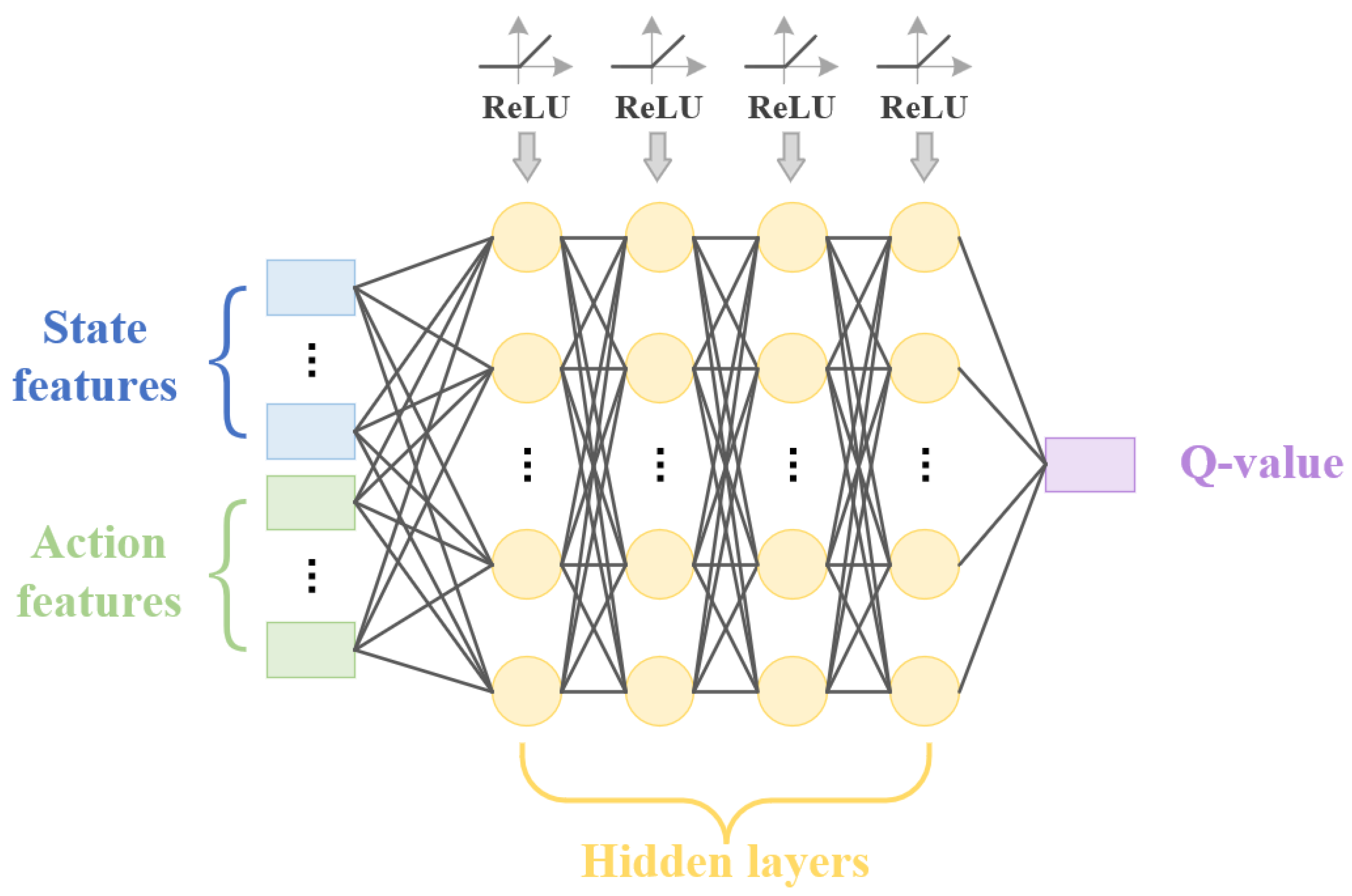
4.2. Action Space

In most studies, the action space usually consists of a set of predefined dispatching rules, the size of which varies from study to study, with the aim of covering as wide a range of decision scenarios as possible. However, in some decision scenarios, the action space cannot fully cover all the scheduling needs of the precast concrete components. This limitation restricts the exploration of potential solutions and can create blind spots in how agents schedule these components, ultimately leading to scheduling solutions that are confined by the predefined rules.

To this end, directly using the set of unscheduled components as the action space will provide the agent with more flexible and comprehensive decision-making space, but it also introduces two main challenges:

(1)

The dynamism of the action space. As production progresses, the number of unscheduled components decreases, leading to a continuously changing size of the action space.

(2)

The dynamic representation of action features. Under different production environment states, scheduling the same component could have varying impacts on the environment. Therefore, the characteristics of actions should evolve with changes in the environmental state.

To address these challenges, this study proposes a new strategy that integrates both environmental state features and individual action features as inputs to the agent, which then outputs a single evaluation value. The agent makes scheduling decisions based on these evaluation values from the unscheduled components. In terms of action feature design, the selected features include the inherent parameter features of the unscheduled components (static) and their processing progress features under the current environment (dynamic). Figure 2 shows the action features, and the specific calculation formulas are shown as follows:

(1)

Proportion of processing time for the unscheduled component relative to the total time

$$S{A}_{1j^{\prime }}={\displaystyle \frac{{\sum }_{p\in P}{t}_{j^{\prime }p}}{{\sum }_{j\in \zeta }{\sum }_{p\in P}{t}_{jp}}}$$

(29)

where $j^{\prime }$ belongs to the unscheduled components’ set.

(2)

Time interval between the completion time of each process of the unscheduled component and the decision point time

$$S{A}_{2j^{\prime }mp}=\left\{\begin{array}{cc}{D}_{j^{\prime }mp}-dt,\hfill & \mathrm{if}\mathrm{process}p\mathrm{of}\mathrm{component}{j}^{\prime }\mathrm{processes}\mathrm{at}\mathrm{workstation}m\hfill \\ 0,\hfill & \mathrm{else}\hfill \end{array}\right.$$

(30)

(3)

Time required to complete the unscheduled component

$$S{A}_{3j^{\prime }}=D_{j^{\prime }m6}-\underset{j\in SCS}{max}\left(D_{jm6}\right)$$

(31)

4.3. Reward Function

Reward serves as the driving force guiding the learning direction of the agent. A well-designed reward function should be closely related to the optimization objective. In this study, the optimization goal for PCC production scheduling problem is to minimize Maxspan. However, minimizing Maxspan in MDP falls into the category of sparse rewards, meaning Maxspan can only be determined after the last component is completed. To promote effective training during non-terminal steps, it is necessary to transform the problem-solving objective, i.e., indirectly map the reward, to facilitate the learning process.

The existing research has shown that minimizing Maxspan can be transformed into maximizing the average utilization rate of workstations. The change in the average utilization rate of workstations at each decision point can reflect the quality of the decision made. Therefore, the change in the average utilization rate of workstations can be used as an immediate reward, expressed as follows:

$$U_{\mathrm{ave}}\left(t\right)=\sum _{k=1}^m{\displaystyle \frac{{\sum }_{j\in SCS\left(t\right)}{\sum }_{p=1}^6{x}_{jmp}·t_{jp}}{m{max}_{j\in SCS\left(t\right)}\left(D_{jm6}\right)}}$$

(32)

$$R_1\left(t\right)=U_{\mathrm{ave}}\left(t\right)-U_{\mathrm{ave}}(t-1)$$

(33)

where $U_{\mathrm{ave}}\left(t\right)$ denotes the average utilization rate of workstations at decision time t, $R_1\left(t\right)$ denotes the immediate reward in the current stage.

Furthermore, the production efficiency of components is closely related to Maxspan. If the average production efficiency of the production line increases, the overall production progress will also accelerate, contributing to the earlier completion of the last components’ production. Therefore, this study further introduces the average production efficiency of the production line as another factor in the reward function. Let $G_{\mathrm{ave}}\left(t\right)$ represents the average production efficiency of the production line at decision time t, $G_{\mathrm{ave}}(t-1)$ represents the average production efficiency in previous stage. The immediate reward $R_2\left(t\right)$ at decision time t can be formulated as:

$$G_{\mathrm{ave}}\left(t\right)={\displaystyle \frac{\left|SCS\right(t\left)\right|+1}{⌊\frac{\underset{j\in SCS\left(t\right)}{max}\left(D_{jm6}\right)}{24}⌋+1}}$$

(34)

$$R_2\left(t\right)=G_{\mathrm{ave}}\left(t\right)-G_{\mathrm{ave}}(t-1)$$

(35)

Therefore, the total immediate reward $R\left(t\right)$ can be defined as:

$$R\left(t\right)=R_1\left(t\right)+R_2\left(t\right)$$

(36)

4.4. Network Structure

The agent in this study is a deep neural network composed of a 4-layer Feedforward Neural Network (FFNN). Both the environmental-state features and the action-state features are fed into the network as inputs, while the output layer generates a single action-evaluation value. At each decision-making step, the agent evaluates each component within the action space and selects the component with the highest evaluation value to be scheduled next, thereby adapting to the dynamic change in the action space. The activation function is ReLU. The structure of the model is shown in Figure 3.

4.5. Overall Framework of the Training Method

The training method is based on the Double Deep Q-Network (DDQN) algorithm framework, which enhances traditional Deep Q-Networks (DQN) by decoupling action selection and value estimation to reduce overestimation bias. Algorithm 2 illustrates the implementation of DDQN in the AO-DRL context, highlighting the interaction between the agent and the environment. During the exploration process, a decision point is defined as the time when a workstation for p2 becomes available. At this decision point, the agent selects the next component to process from the unscheduled components’ set (UCS) based on the 3-greedy policy, receives an immediate reward, transitions to the next state, and stores the experience tuple (state, action, reward, next state, UCS) into the replay buffer. In the model training phase, experience replay is utilized to sample minibatches of experiences, compute the loss between the online network Q and the target network $\widehat{Q}$, and update the parameters of the online network using gradient descent. Additionally, the target network parameters are updated every C steps to ensure stable learning.

Algorithm 2 DDQN algorithm framework

1: Initialize experience replay buffer D with capacity N 2: Initialize parameters of online network Q as $\theta$ 3: Initialize parameters of target network $\widehat{Q}$ as $\widehat{\theta }$, where $\widehat{\theta }$ = $\theta$ 4: for epoch = 1 to Nepoch do 5:       Generate N random components with processing time 6:       Initialize state $s_1$ and compute the action features of component j in unscheduled components’ set (USC) 7:       for t = 1 to N do 8:             Select action $a_t$ with probability $\epsilon$ randomly, 9:             otherwise $a_t=\arg {max}_{a\in UCS}Q(s_t,a;\theta )$ 10:           Execute action $a_t$, observe next state $s_{t+1}$, compute reward $r_t$ 11:           Update the action features of component in unscheduled components’ set 12:           Remove action $a_t$ from UCS 13:           Store ($s_t$, $a_t$, $r_t$, $s_{t+1}$, t, UCS) in D 14:           $s_t=s_t$ 15:           Sample minbatch of experiences ($s_j$, $a_j$, $r_j$, $s_{j+1}$, j, UCS’) from D 16:           if epoch terminates at step j then 17:                Set $y_j=r_j$ 18:           else 19:                Set $y_j=r_j+\gamma \widehat{Q}(s_{j+1},\arg {max}_{a^{\prime }\in UC{S}^{\prime }}Q(s_{j+1},a^{\prime };\theta );\widehat{\theta })$ 20:           end if 21:           Perform gradient descent on the loss ${(y_j-Q(s_j,a_j;\theta ))}^2$ to update parameters $\theta$ of online network 22:           Every C steps, update target network’s parameters $\widehat{\theta }=\theta$ 23:       end for 24: end for

5. Experiments

5.1. Basic Conditions

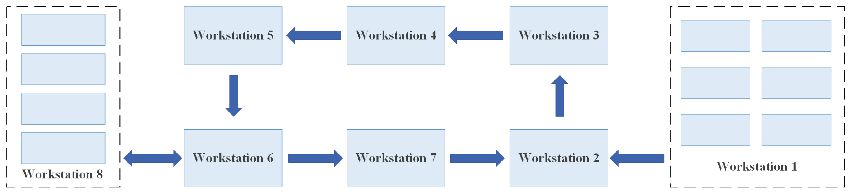
The actual beam-factory production line is employed as the experimental case environment. The layout of the production line is illustrated in Figure 4. Workstations corresponding to each process are detailed in

Table 2. Correspondence between processes and workstations.

Process	p1	p2	p3	p4	p5	p6
Workstation	1	2	2, 3, 4, 5	6	8	6, 7

.

Unlike a serial production line, this line employs a circular layout. Its key feature is that Workstation 1 is responsible for performing two non-continuous processes (p4 and p6). This introduces production conflicts between these processes, making the scheduling problem more complex.

The experimental environment configuration is as follows: Intel Core i5-9400 CPU @ 2.90 GHz, 8 GB RAM, 64-bit Windows 11, and an NVIDIA RTX 3060 GPU. All algorithms were implemented using Python 3.7, with PyCharm 2020 as the development platform, and the deep learning model was built using PyTorch 1.8.

To validate the effectiveness of the proposed method compared with baseline, normalized performance (NP) is used for evaluation. The calculation formula is shown in Equation (37). The positive NP value indicates better performance than the benchmark algorithm.

$$NP={\displaystyle \frac{T_{baseline}-T_{algorithm}}{T_{baseline}}}$$

(37)

where $T_{baseline}$ denotes NP of the benchmark algorithm. $T_{algorithm}$ denotes NP of the competitive algorithm

5.2. The Training Process of AO-DRL

Table 3. Hyperparameter for training AO-DRL.

Hyperparameter	Value
Number of training episodes	250
Replay buffer size	2000
Batch size	32
Exploration Rate	Linearly decreased from 0.9 to 0.01
Discount factor	0.95
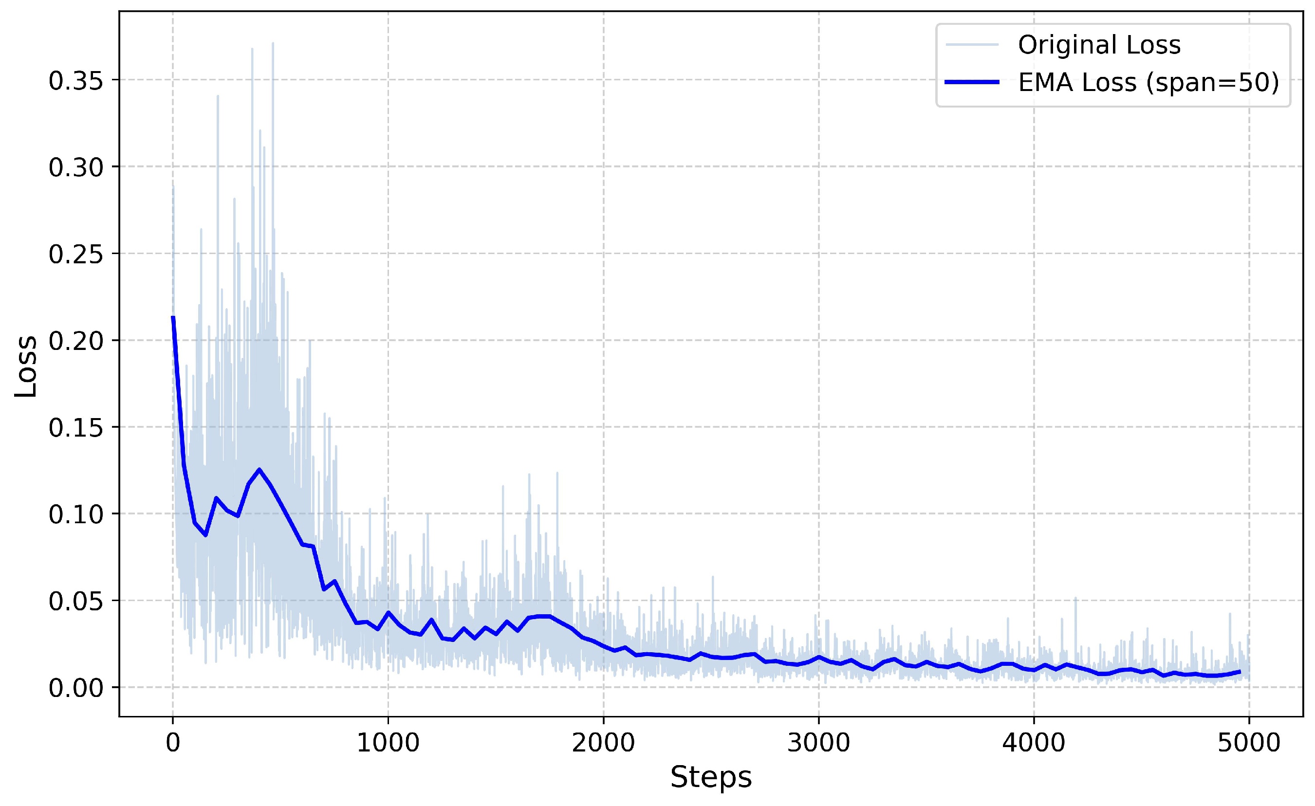
Target network update frequency	20

presents the parameter configuration for training AO-DRL. During each episode of training, 20 components are randomly selected from historical data to form a training sample. The test set consists of 5 samples, each containing 20 components, and remains fixed throughout the entire training process. The performance of AO-DRL is evaluated by calculating the Maxspan sum of the agent on the test set, which helps to assess the training effectiveness and mitigate the influence of random factors.

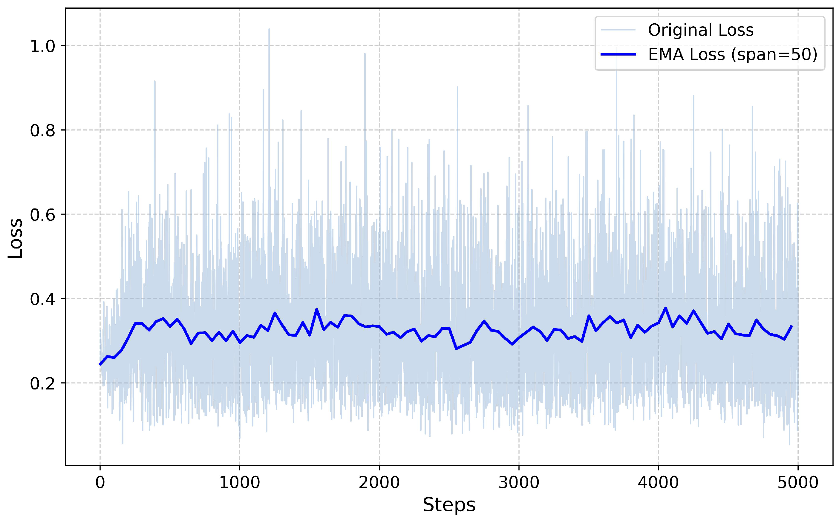
Figure 5 illustrates the loss curve of the agent during the training period. From the figure, it can be observed that in the initial stages of training, the loss value shows a high and increasing trend. This is due to the random initialization of neural network parameters, where the agent has not yet learned effective policy information. Additionally, the updates to the Q-network can cause fluctuations in the loss value due to the varying distribution of samples. As training progresses, the loss value exhibits a rapid downward trend, indicating that the agent accumulates more experience data through continuous interaction with the environment and gradually adjusts its policy to better adapt to the environment. In the later stages of training, the loss value demonstrates a reduction in fluctuations and stabilizes at a lower level, suggesting that the agent’s learning process has reached a convergent state.

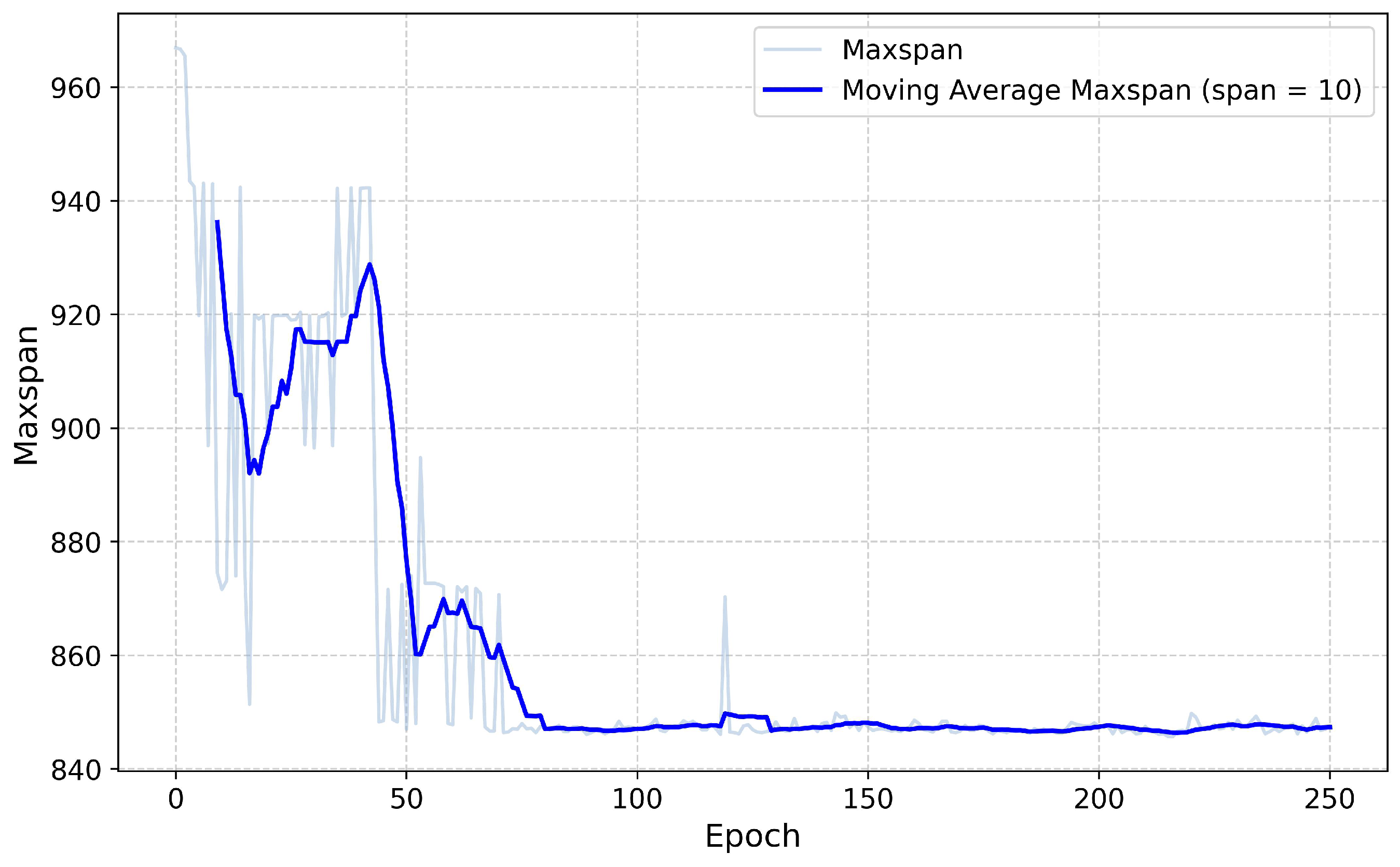
Figure 6 illustrates the change in the Maxspan sum on the test set during the agent’s training process. The red line represents the moving average of the Maxspan sum on the test set from the previous 10 steps to the current step. The training results show that, as the training progresses, the Maxspan sum received by the agent on the test set exhibits a fluctuating downward trend. This further indicates that the agent has achieved good performance in solving the problem of minimizing the Maxspan for PCC production.

5.3. Comparison with RO-DRL

The action space of RO-DRL consists of four common single-dispatching rules, as shown in

Table 4. Dispatching rules.

No.	Dispatching Rule	Description
1	SPT	Schedule the component with the shortest processing time first.
2	EFT	Schedule the component that will finish production the earliest.
3	MUR	Schedule the component that maximizes the utilization rate of the workstations.
4	LFT	Schedule the component that will finish production the latest.

. The model accepts the state features of the production line environment as input and outputs an evaluation value that matches the action space size. When the highest evaluation value corresponds to multiple precast concrete components, a component is selected randomly. RO-DRL is trained using the same experimental case environment as the proposed approach, and both approaches share the same parameter configurations.

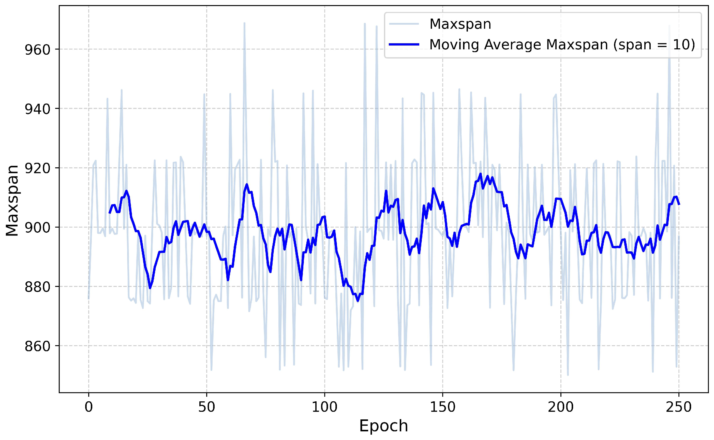
Figure 7 and Figure 8 illustrate the changes in the loss values and Maxspan sum during the training process of RO-DRL. It can be observed that the RO-DRL exhibits significant and sustained oscillations in both loss values and Maxspan sum during training process. This indicates that the model fails to achieve stable convergence and has not learned effective strategies for PCC production scheduling.

The main reason for this problem is that the RO-DRL primarily selects the optimal dispatching rule from a macro perspective to determine the order in which the components enter the production line. However, due to the characteristics of the PCC problem in this study, the specific scheduling arrangements of components after they enter the production line are handled by Algorithm 1. These micro-level decision details affect the macro-level state of the production line environment but cannot be fed back to the RO-DRL. Consequently, due to this difference between the macro and micro perspectives, the RO-DRL model struggles to accurately model the relationship between the state features of the production line and the dispatching rules, thereby impacting the convergence of the approach and the effectiveness of its policies.

5.4. Comparison with Competitive Algorithms

This section evaluates the performance of the proposed approach against baseline methods. The baseline methods include genetic algorithm (GA), DQN, and three dispatching rules: SPT(Rule1), EFT(Rule2), MUR(Rule3) listed in Table 4. The primary distinction between AO-DRL and DQN lies in that AO-DRL employs dual independent Q-networks for action-value function estimation and action selection, respectively, while other parameter configurations remain consistent between the two approaches.

For the experiments, 20 random samples, each containing 10 components, are generated to test these approaches’ performance. Both AO-DRL and DQN are trained in an environment with 10 components to develop the optimal agent.

Table 5. Performance comparison of different methods.

No.	AO-DRL	DQN	GA	Rule 1	Rule 2	Rule 3
1	97.1 * (0.21%↓)	97.1 * (0.21%↓)	96.9 **	97.1 * (0.21%↓)	99.0 (2.17%↓)	98.5 (1.65%↓)
2	97.5 * (0.62%↓)	97.5 * (0.62%↓)	96.9 **	97.5 * (0.62%↓)	97.5 * (0.62%↓)	96.9 **
3	98.2 (1.24%↓)	97.8 (0.42%↓)	97.0 **	97.4 (0.41%↓)	99.1 (2.16%↓)	97.1 * (0.10%↓)
4	97.0 * (0.10%↓)	97.1 (0.21%↓)	96.9 **	97.1 (0.21%↓)	97.5 (0.62%↓)	97.0 * (0.10%↓)
5	97.0 **	97.2 * (0.21%↓)	97.0 **	97.5 * (0.52%↓)	99.1 (2.16%↓)	98.6 (1.65%↓)
6	98.4 **	98.8 * (0.41%↓)	99.2 * (0.81%↓)	99.4 (1.02%↓)	101.8 (3.46%↓)	100.1 (2.74%↓)
7	97.0 **	97.0 **	97.0 **	97.3 * (0.31%↓)	97.5 (0.52%↓)	98.0 (1.03%↓)
8	97.0 * (0.10%↓)	97.0 *	96.9 **	97.2 (0.31%↓)	97.5 (0.62%↓)	96.9 **
9	98.6 (0.61%↓)	98.6 (0.61%↓)	98.0 **	98.5 (0.51%↓)	99.1 (1.12%↓)	98.1 * (0.1%↓)
10	96.9 **	96.9 **	96.9 **	97.0 * (0.10%↓)	99.0 (2.17%↓)	97.2 (0.31%↓)
11	97.1 * (0.10%↓)	97.1 * (0.10%↓)	97.0 **	97.3 (0.31%↓)	97.5 (0.62%↓)	97.0 **
12	99.4 * (1.02%↓)	99.4 * (1.02%↓)	98.4 **	99.6 (1.22%↓)	100.4 (%↓)	99.5 (1.12%↓)
13	97.0 **	97.0 **	97.0 **	97.4 (0.41%↓)	98.8 (1.86%↓)	97.2 * (0.21%↓)
14	98.1 * (1.13%↓)	98.1 * (1.13%↓)	97.0 **	98.6 (1.65%↓)	100.5 (3.61%↓)	98.5 (1.55%↓)
15	96.9 **	96.9 **	96.9 **	97.4 * (0.52%↓)	97.6 (0.72%↓)	96.9 **
16	98.3 **	98.6 * (0.31%↓)	98.3 **	98.3 **	98.6 * (0.31%↓)	99.8 (1.53%↓)
17	97.1 * (0.21%↓)	97.2 (0.31%↓)	96.9 **	98.4 (1.55%↓)	97.5 (0.62%↓)	97.2 (0.31%↓)
18	97.1 * (0.10%↓)	97.1 * (0.10%↓)	97.0 **	97.4 (0.41%↓)	97.6 (0.62%↓)	97.0 **
19	97.4 * (0.41%↓)	98.4 (1.41%↓)	97.0 **	98.4 (1.44%↓)	99.1 (2.16%↓)	98.2 (1.24%↓)
20	98.3 * (0.31%↓)	98.3 * (0.31%↓)	98.0 **	98.9 (0.92%↓)	99.2 (1.22%↓)	99.0 (1.02%↓)

Note: ** marks the best result obtained in the case samples. * marks the second-best result obtained in the case samples. ↓ marks the performance gap with the best result.

presents the experimental results for AO-DRL, DQN, GA, and the three dispatching rules under 10-scale-jobs.

The experimental results show that AO-DRL outperforms the other three dispatching rules in the most test samples. Compared to DQN, AO-DRL achieves a performance improvement by decoupling action selection from target computation, thereby reducing estimation instability and bias, which ultimately enhances the final performance of AO-DRL. Although the overall performance of AO-DRL is slightly inferior to that of GA, which requires longer computation times, the performance gap between AO-DRL and GA is generally maintained within about 1%. Moreover, in the cases where AO-DRL achieves the best results, AO-DRL can even outperform GA, with an improvement rate also within 1%.

To further investigate the differences in solution quality between between AO-DRL and GA on larger-scale problems, two additional experiments are designed, focusing on scenarios with 20 components and 30 components, respectively. Each experiment involves generating 20 random test samples to evaluate the performance of both algorithms.

Table 6. Comparison of AO-DRL and GA on different-scale tasks.

Job-Scale	GA		AO-DRL
	Maxspan (h)	CPU (s)	95% Confidence Interval	Maxspan (h)	CPU (s)	95% Confidence Interval
10	97	159.57	[97.0, 97.6]	98.2 (1.2%↓)	1.08	[97.2, 97.9]
	99.2	162.31		98.4 (0.8%↑)	1.00
20	146.4	584.46	[147.4, 155.8]	147.4 (0.7%↓)	5.97	[147.5, 156.0]
	147.3	594.59		146.9 (0.3%↑)	6.14
30	241.5	1241.33	[217.9, 225.7]	242.9 (0.6%↓)	18.94	[216.2, 225.8]
	216.9	1228.67		196.4 (9.5%↑)	18.99

Note: ↑ marks the performance improvement with the GA result. ↓ marks the performance gap with the GA result.

presents the key performance metrics, including the average solving time, the best and worst solutions obtained by each algorithm, along with the 95% confidence intervals.

The experimental results show that as the task scale increases, the performance gap in Maxspan between AO-DRL and GA narrows in the samples where AO-DRL reaches the worst solutions. This gap decreases from 1.2% to 0.6%. In the cases where the best solutions are obtained, the proposed approach also shows a slight performance improvement over GA. Notably, in the 30-components scenario, AO-DRL outperforms GA by a significant improvement of 9.5%. It is primarily attributed to the fact that the search space for GA grows exponentially with increasing task scale, making it more difficult to find the global optimum and leading to a higher risk of getting trapped in local optima. In contrast, AO-DRL can dynamically adjust its scheduling strategy based on the current state of the environment and continuously refine it through ongoing interaction with the environment. This makes the exploration of the solution space more efficient, helping to find better solutions and thus significantly outperforming GA in certain scenarios.

From the perspective of the 95% confidence intervals, there is considerable overlap between the intervals of AO-DRL and GA across different problem scales. This suggests that there is no statistically significant difference in performance between the two algorithms, indicating that their performance is relatively similar in terms of solution quality.

Additionally, the analysis of computational resource consumption shows that the solving time for both AO-DRL and GA increases as the task scale grows. However, the AO-DRL demonstrates a significant advantage in solving speed compared to GA, reducing the solving time by several orders of magnitude. This is particularly important for handling large-scale scheduling problems.

5.5. Generalization Performance Analysis

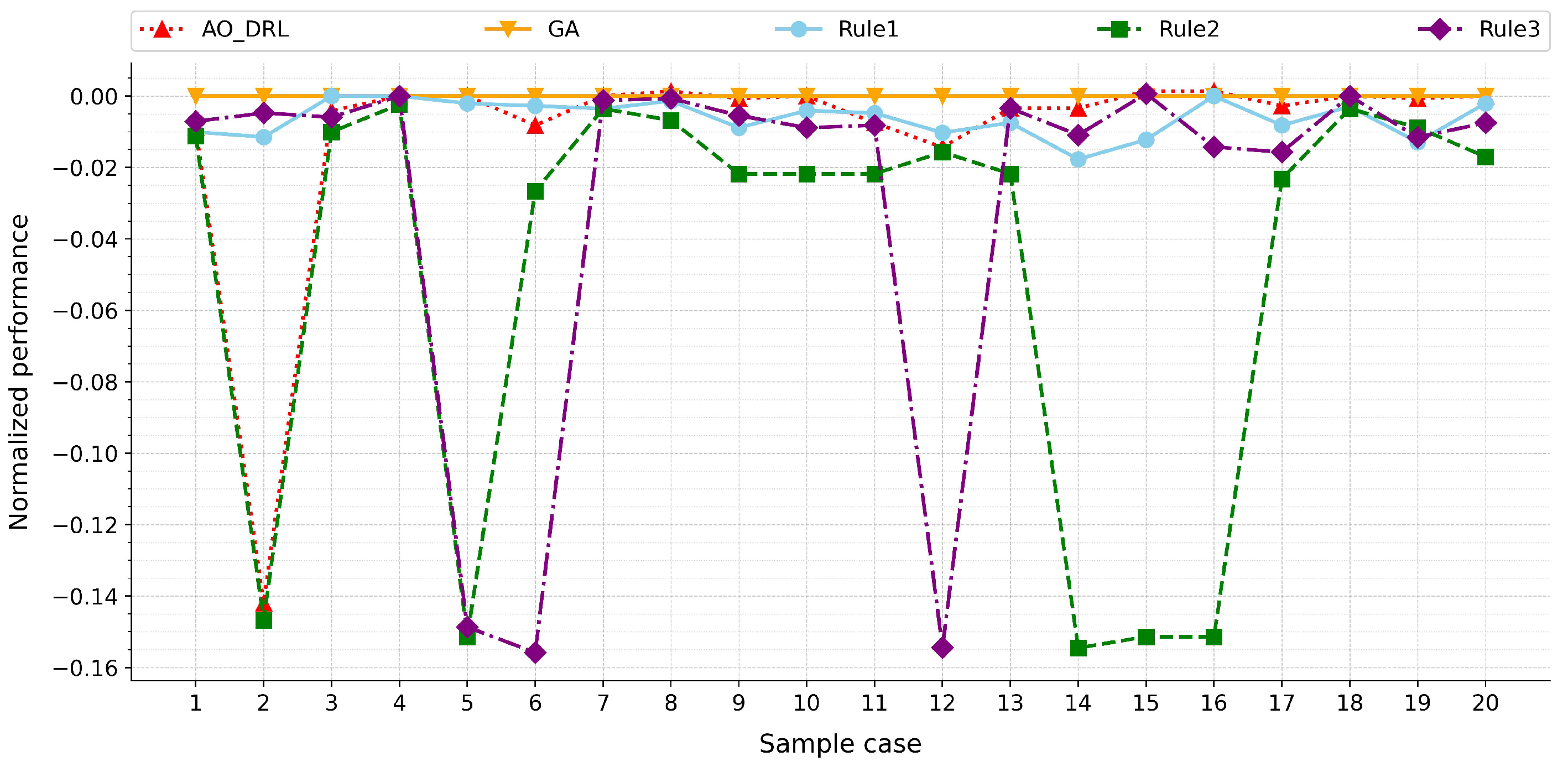
To further investigate the generalization performance of the proposed approach, this section applies the AO-DRL to samples that exceed the scale of the training set. Specifically, the AO-DRL is first trained using samples with 10 components. After training, the model is tested on datasets with 20 and 30 components to evaluate its generalization capability. Each test set contains 20 samples.

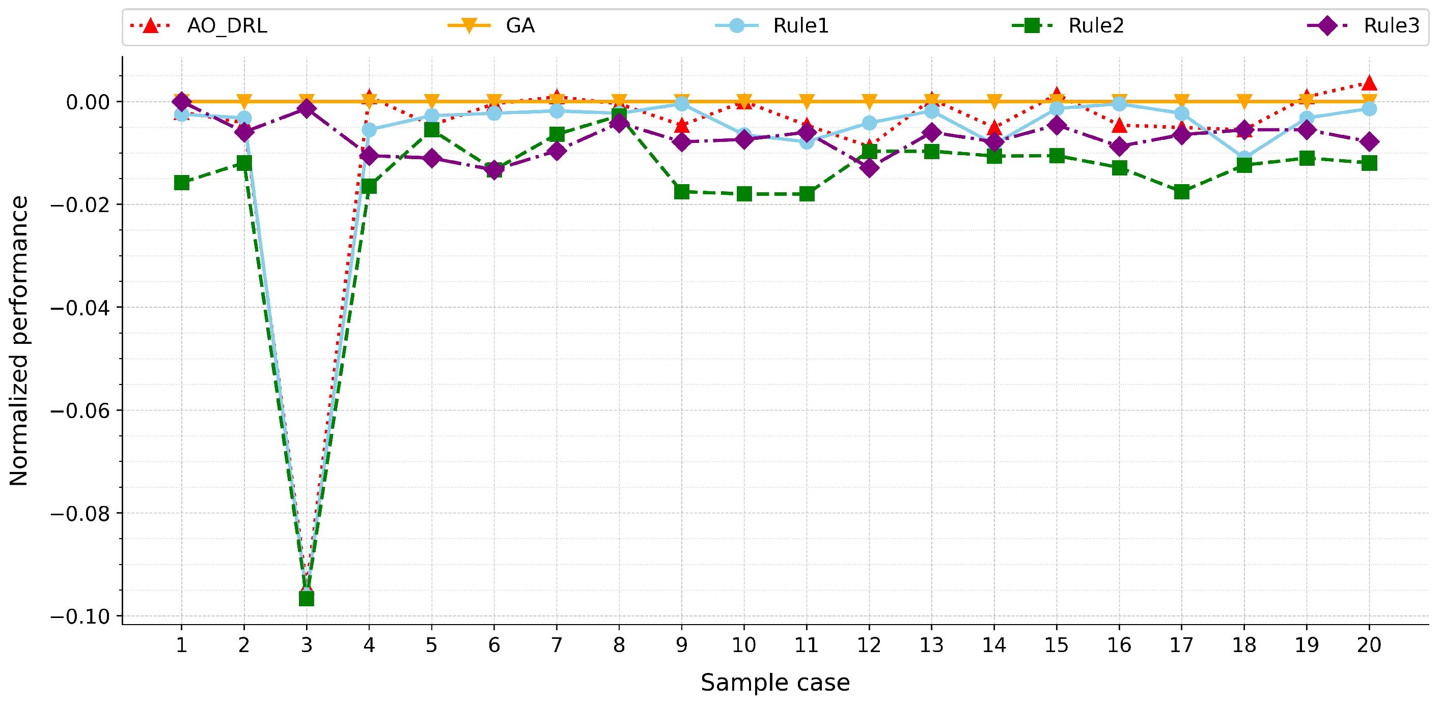
To compare the performance gaps among different methods, the performance of all methods is normalized using Equation (37), where the results of the genetic algorithm (GA) are used as the benchmark performance. The performance comparison charts are shown in Figure 9 and Figure 10. In these figures, the benchmark performance of GA is indicated by a bold orange line, while the normalized performance of AO-DRL is represented by a bold red line.

From Figure 9 and Figure 10, it can be observed that AO-DRL, trained on small-scale instances, consistently outperforms traditional dispatching rules in most samples, with the performance-gap improvement ranging from 0.6% to 3.8%. Although there is a certain performance gap compared to GA, the gap is relatively small, averaging within 2%. However, it is also noted that in specific cases (e.g., Case 2 in Figure 9 and Case 3 in Figure 10), the performance gap increases significantly, reaching 14% and 8%, respectively. This may occur due to the lack of similar data distributions in the training phase, leading to insufficient decision-making capabilities of AO-DRL when dealing with such specific data.

A combined analysis of Figure 9 and Figure 10 reveals that as the problem scale increases, the performance gap between AO-DRL and GA exhibits a decreasing trend. This is because, as the problem scale grows, the performance of the solution becomes more focused on the overall rationality of the approach. Therefore, this trend suggests that AO-DRL’s performance becomes more competitive as the problem complexity increases, highlighting its potential for scalability in larger-scale scheduling tasks.

6. Discussion

6.1. Analysis Between AO-DRL and RO-DRL

Through the experimental comparisons in Section 5.2 and Section 5.3, it can be observed that the differences in scheduling strategies between RO-DRL and AO-DRL have a considerable impact on the the experimental results. The possible reasons are mainly attributed to the following aspects:

(1)

Special Characteristics of the Problem

Previous research on FSP often focuses on process-level scheduling, where each process step is treated as an independent decision point. The results can be immediately fed back to the agent, ensuring the continuity and immediacy of decision information. In such an environment, RO-DRL effectively establishes a close relationship between the environment and the rules. However, this study addresses job-level scheduling, which means the focus of decision-making is on determining the production sequence of PPCs. The specific scheduling information for each process step within a component is not fed back to the agent, leading to discontinuity in decision information.

(2)

Action Space Design

The AO-DRL defines the action space as the set of unscheduled components, which avoids the complex design of dispatching rules and provides the agent with a more intuitive and comprehensive decision-making space. Additionally, the introduction of action features in AO-DRL directly provides the agent with current scheduling information for the process within the component, effectively overcoming the issue of information fragmentation. Consequently, AO-DRL demonstrates higher stability and performance in the experiment.

6.2. Analysis Between AO-DRL and GA

According to the experimental results presented in Section 5.4 and Section 5.5, despite a slight gap in the Maxspan compared to GA, AO-DRL demonstrates significant advantages when handling larger-scale problems:

(1)

Solution Efficiency and Cost

As the complexity of the problem increases, the solving time and computational cost for GA rise significantly, potentially preventing it from providing satisfactory solutions within a given time. In contrast, AO-DRL leverages reinforcement learning to learn and understand the direct interaction patterns between the environment states and PCC scheduling. This enables AO-DRL to find a better solution within limited decision cycles.

(2)

Adaptability and Generalization

When the problem scale changes, GA requires reiterative processes of encoding and decoding tasks. However, due to its network structure, AO-DRL can flexibly adapt to the dynamically changing action space. Additionally, AO-DRL’s strong generalization capability allows it to quickly adjust strategy based on the existing decision foundation, enabling rapid rescheduling in response to unseen events. However, the experimental result in Section 5.5 also reveals a significant performance degradation for AO-DRL when generalized to large-scale problems. To address this challenge, an ensemble learning strategy can be adopted, integrating AO-DRL with selected dispatching rules to enhance the robustness of the solution.

6.3. Practical Application Limitations of AO-DRL

In practical applications, AO-DRL encounters two primary challenges:

(1)

Dependency on Environmental Layout

As demonstrated in Section 4.1 and Section 4.2, some of the state features and action features are closely associated with the specific layout of production environments. This design allows the agent to capture detailed characteristics of the production environment, thereby providing comprehensive information for decision making. However, it also leads to a high dependency on specific environmental layouts, limiting the model’s applicability across different environments.

(2)

Generalization challenges with large-scale problems.

The experimental results in Section 5.5 reveal a significant performance degradation for AO-DRL when generalized to large-scale problems. This is mainly attributed to the discrepancy in sample distribution between small-scale training samples and large-scale tasks, leading to biased decision-making strategies when the model addresses large-scale problems, thus affecting its generalization capability.

To mitigate these limitations, some strategies can be employed to enhance AO-DRL performance. For example, ensemble learning methods improve overall performance by aggregating the outcomes of multiple algorithms or models. For AO-DRL, this can be achieved by integrating decisions from agents trained on smaller scales with preferred scheduling rules, thereby compensating for deficiencies in individual approaches and enhancing the robustness and reliability of the results.

In addition, curriculum learning is a progressive training approach that starts with simpler tasks and gradually transitions to more complex ones. Therefore, the training process for AO-DRL can begin with smaller-scale tasks (e.g., 10 components) to acquire foundational decision-making strategies, and gradually increase to larger-scale tasks (such as 20, 50, and 100 components) according to the learning progress, further enhancing the model’s adaptability and robustness.

7. Conclusions

This study proposes AO-DRL to address the production scheduling problem of PCC, specifically aimed at minimizing Maxspan. To ensure that the proposed model remains relevant and applicable to real-world production scenarios, various practical constraints are considered within the model. These include workstation transitions, transfer times, overtime considerations, parallel and serial workstations, and the absence of buffer zones.

The innovation of this study lies in the design of the AO-DRL. The approach defines the set of unscheduled components as the action space, thereby avoiding the complexity of designing dispatching rules. By taking state features and action features as joint inputs, the agent can evaluate the Q-value of each unscheduled component under the current environment. Based on these evaluations, the agent can make more direct and comprehensive scheduling decisions.

Experimental results show that the proposed AO-DRL effectively solves the issue of information fragmentation during the decision-making process and outperforms rule-based scheduling methods in minimizing Maxspan, with an average superiority rate exceeding 80%. Compared to GA, AO-DRL maintains solution quality with only a 1% gap while significantly improving computational efficiency by orders of magnitude. Additionally, generalization performance experiments indicate that AO-DRL exhibits robust generalization capabilities, maintaining high solution quality on an untrained large-scale problem. This enables AO-DRL to rapidly generate near-optimal scheduling plans, making it highly suitable for time-sensitive real-world applications. Its robustness in handling problems of varying scales and complexities further enhances its applicability across diverse production environments.

However, there remain certain limitations within this study. AO-DRL exhibits a strong dependency on the layout of the production environment. When unforeseen changes occur within the environment, such as a reduction in workstations or equipment failures, the performance of the model may be affected. Future research should focus on: (1) applying the approach to more uncertain, constrained scheduling circumstances, such as machine failures and automated guided-vehicle malfunctions; (2) exploring the application of reinforcement learning in fine-grained scheduling of the process to reduce the occurrence of “phantom congestion”.