Identifying Damage in Structures: Definition of Thresholds to Minimize False Alarms in SHM Systems

Abstract

In recent years, the development of quick and streamlined methods for the detection and localization of structural damage has been achieved by analysing key dynamic parameters before and after significant events or as a result of aging. Many Structural Health Monitoring (SHM) systems rely on the relationship between occurred damage and variations in eigenfrequencies. While it is acknowledged that damage can affect eigenfrequencies, the reverse is not necessarily true, particularly for minor frequency variations. Thus, reducing false positives is essential for the effectiveness of SHM systems. The aim of this paper is to identify scenarios where observed changes in eigenfrequencies are not caused by structural damage, but rather by non-stationary combinations of input and system response (e.g., wind effects, traffic vibrations), or by stochastic variations in mass, damping, and stiffness (e.g., environmental variations). To achieve this, statistical variations of thresholds were established to separate linear non-stationary behaviour from nonlinear structural behaviour. The Duffing oscillator was employed in this study to perform various nonlinear analyses via Monte Carlo simulations.

1. Introduction

The safety and functionality of structures can be significantly compromised by the loss of structural integrity due to gradual aging, deterioration, or critical events such as earthquakes, explosions, and hurricanes. It is crucial to detect structural damage as early as possible to prevent catastrophic outcomes. Structural Health Monitoring (SHM) aims to fulfil this requirement [1]. The process involves detecting the occurrence of damage, identifying its location, and assessing its severity. These steps can be supported through various Non-Destructive Testing (NDT) methods [2], including visual inspection, digital image correlation, ultrasound, acoustic emission, magnetic field, eddy current, thermography, and radiography, among others. Typically, these experimental techniques are localized methods [3] capable of inspecting only a limited area at a time, necessitating multiple measurements to thoroughly inspect a structure or to focus on specific regions. Such NDT techniques also require that the section of the structure being inspected is readily accessible [4,5,6]. The demand for quantitative global damage detection has led to the development of two global methods. One is based on the measurement of static deflections [7,8], and the other on changes in the vibration characteristics of structures, namely, vibration-based damage detection methods. In the vibration-based method, damage detection is achieved by examining changes in the measured vibration response, where the modal parameters (natural frequencies, mode shapes, and modal damping) are indicative of the physical properties (mass, damping, and stiffness) of a structure [9]. Thus, changes in structural properties result in changes in modal properties [10,11,12], which can be detected either absolutely or more often by comparison to an undamaged state. Vibration-based damage detection has garnered significant attention, with a variety of methods proposed over recent decades, ranging from those based on changes in modal parameters to those incorporating signal processing, model updating, and optimization algorithms. Doebling et al. [9] provided an overview of damage detection methods based on changes in basic modal properties (e.g., natural frequencies, mode shapes, and modal damping ratios) up to 1998. A review of subsequent literature indicates that many of the issues summarized in [9], such as the dependence on prior test data and linear structural models, the number and location of measurement sensors, and the sensitivity to minor flaws, remain unaddressed and are still subjects of ongoing research across the community. In scenarios of multiple cracking, where cracking progresses, the impact of cracking on the dynamic response is primarily influenced by the extent of cracking. The author suggested that to successfully detect cracks of various severity, the use of advanced signal processing techniques, such as the wavelet transform and the Hilbert–Huang transform, should be considered. Although advanced signal processing is not the central focus of the current review, relevant recent applications are included. In 2011, a review of vibration-based damage identification methods was conducted by Fan and Qiao [13], classifying the methods into four categories: natural frequency-based, mode shape-based, modal curvature-based, and combined methods based on both frequencies and mode shapes. In 2015, a review specifically focused on wavelet analysis of modal curvatures for composite structures was conducted by Katunin [14], discussing the influence of various factors such as measurement apparatus, measurement noise, wavelet functions, damage location, sampling distance, and boundary effects. To overcome some limitations derived from the use of classical tools to analyse the time-varying behaviour of damaging structures, in 2012 [15], a band-variable filter based on the Stockwell transform [16] was proposed to accurately evaluate eigenfrequencies and related mode shapes of damaging structures during the strong motion phase. In 2015, a novel tool [17] was proposed to automatically evaluate the equivalent viscous damping factor associated with the fundamental mode of vibration before, during, and after an earthquake. Ditommaso et al. [18] proposed a methodology for damage localization based on the band variable filter, which has been applied in both numerical and experimental case studies. Iacovino et al. [19] proposed a variation of the Curvature Evolution Method (CEM), aiming to reduce some uncertainties derived from the evaluation of modal parameters during a strong-motion earthquake. The CEM method for damage location was updated by Ditommaso et al. [20] and successfully applied to a damaged structure [20,21], providing the possibility of also quantifying structural damage by defining empirical correlations between curvature variation and maximum inter-story drift (valid only for reinforced concrete framed structures). In recent years, the reduction in the cost of structural monitoring technologies has promoted their widespread adoption for both building and infrastructure monitoring. Among the various sensor types on the market, monitoring systems based on vibration data analysis are the most prevalent and are generally based on data acquired from velocity and/or acceleration sensors. The market introduction of increasingly high-performance, low-cost sensors is promoting their widespread adoption. As discussed above, a vibration-based structural monitoring system relies on comparing the dynamic characteristics of the system evaluated at a given time with those exhibited by the system at a reference time. The reliability of comparing dynamic parameters increases with the accuracy of their estimation under both steady-state and transient conditions. An incorrect estimate of parameter variations can lead to incorrect assessments of a construction’s health status, with possible repercussions on occupant safety and significant implications in terms of the direct and indirect costs associated with potential false alarms. While changes in mechanical properties produce changes in structural eigenfrequencies, the reverse is not always true, especially for minor variations [22,23,24,25]. Frequency variations fall into two categories: long-term and short-term. Long-term changes can be caused by factors like temperature fluctuations, which can sometimes surpass the effects caused by variations in structural parameters [26,27], or moisture changes in the foundation soil [28,29,30,31,32]. Short-term fluctuations, on the other hand, are typically observed during critical events. However, the system’s response might also exhibit apparent changes due to impulsive phenomena like traffic, wind, or minor earthquakes. Today, as we aim to implement intelligent systems capable of automatically providing an estimate of the condition of the monitored structure and deciding whether or not to raise an alarm, the issue is becoming increasingly relevant. In this context, it is important to use algorithms based on threshold-based analysis techniques to accurately establish the health status of monitored structures [33]. Starting from the understanding that the likelihood of incorrectly assessing the presence of damage is less in the case of critical events of considerable intensity, such as strong earthquakes, from the perspective of developing automatic systems for damage assessment, it is also crucial to reduce the uncertainties related to the variation in vibration frequencies related to phenomena not necessarily indicative of damage. Figure 1 shows an example of minor frequency variations observed on a real accelerometer acquisition performed on an operational bridge under normal conditions [34].

In this regard, the small frequency variations can be linked to many phenomena such as, for example, the combination of input and transient response of the system, the opening and closing of cracks and micro-cracks, and the nonlinearities due to interaction between the various structural and non-structural components. It is clear that the combination of all these effects cannot be evaluated deterministically from the solution of the differential equations of motion but can be evaluated statistically using a dynamic model able to take into account the onset of small nonlinearities and also small variations in mass, stiffness, and damping that can characterize the response of real systems under operating conditions.

Finally, considering that each vibration mode of a dynamic system can be modelled as a Single-Degree-of-Freedom (SDOF) oscillator, the Duffing model implemented in MATLAB^® was used to perform Monte Carlo simulations in order to find, using a statistical approach, the behavioural thresholds of the system that can distinguish the onset of damage from other non-stationary phenomena.

2. Analysis of the Problem

The study of a Single-Degree-of-Freedom (SDOF) system is not only a tool for the analysis of simple structural systems but also enables the study and understanding of the dynamic behaviour of more complex systems. The simplest SDOF system available is an elementary oscillator where the principle dynamic characteristics are concentrated in three distinct elements: the mass m of the system, the stiffness k of the elastic spring, and the constant c synthetically representing all forms of system dissipation. The forces which balance dynamic action are the inertia force $f_I=m·\ddot{u}\left(t\right)$, the viscous force $f_D=c·\dot{u}\left(t\right)$, and the recentring elastic force $f_S=k·u\left(t\right)$. External actions are represented by the load p(t). Applying D’Alembert’s Principle, the equation of motion is formulised as follows:

$$m·\ddot{u}\left(t\right)+c·\dot{u}\left(t\right)+k·u\left(t\right)=p\left(t\right)$$

(1)

where m, c, and k represent the mass, the damping, and stiffness of the system, respectively.

In this case (Equation (1)), it is possible to evaluate the settling time of a system using the following equation (neglecting the amplitude of the solution when it becomes less than one per cent of the initial amplitude):

$$t_{ass}=\frac{4.61}{\xi {\omega }_0}\left[\mathrm{Settling}\mathrm{time}\mathrm{of}\mathrm{the}\mathrm{system}\right]$$

(2)

where

${\omega }_0=\sqrt{\frac{k}{m}}$ is the natural circular frequency of the system;

$\xi =\frac{c}{2\cdot m·{\omega }_0}$ is the equivalent viscous damping ratio.

When a transient response is generated by a force with a frequency different from the self-frequency of the monitored system, it is easy to distinguish the frequency of the system during the transient phase from the frequency of the forcer during the stationary phase (Figure 2). However, if the forcing has a frequency close to that of the monitored system and lasts longer than the settling time, as happens often on real systems due to anthropogenic and environmental inputs, there is a risk of confusing the frequency of the structure with the frequency of the forcing during the transition phase.

The same risk arises when the forcing stops, and the system undergoes another transient phase before returning to free oscillations. On a perfectly elastic system, apparent variations in frequency can be continuously generated. However, this occurs only at the particular combination of input and response during the transition from the transient phase to the stationary phase and vice versa. This mechanism repeats itself an unlimited number of times during the life of a structure and does not create any structural problems [35]. However, it can cause confusion in the interpretation of vibrational data (an example is depicted in Figure 3) where the effect of the phenomenon is extremized.

Figure 3 shows that the transition between phases (transient to stationary and vice versa) occurs continuously. This continuity could be misleading for the monitoring system or the user analysing the data because there are currently no criteria to determine whether the observed frequency variations are correlated to damages or generated by non-stationary mechanisms. In this work, with the aim to also consider slight nonlinearities on the SDOF system, the Duffing stiffness [36] was considered and the equation was modified as follows:

$$m·\ddot{u}\left(t\right)+c·\dot{u}\left(t\right)+k·u\left(t\right)+\beta ·{u\left(t\right)}^3=f\left(t\right)$$

(3)

where $\beta$ can be considered as the coefficient of cubic stiffness of the SDOF system. This kind of equation has been widely used to analyse the chaotic behaviour of oscillating systems exciting both from stationary and stochastic input motion [37,38,39]. Graphically, the SDOF system of Equation (3) can be represented with the scheme depicted in Figure 4.

For Equation (1), the solution is obtained from the sum of an associated homogenous solution (the known zero state) and a particular solution of the complete equation. From a physical point of view, the superposition of two independent terms corresponds to the superposition of the following two phenomena:

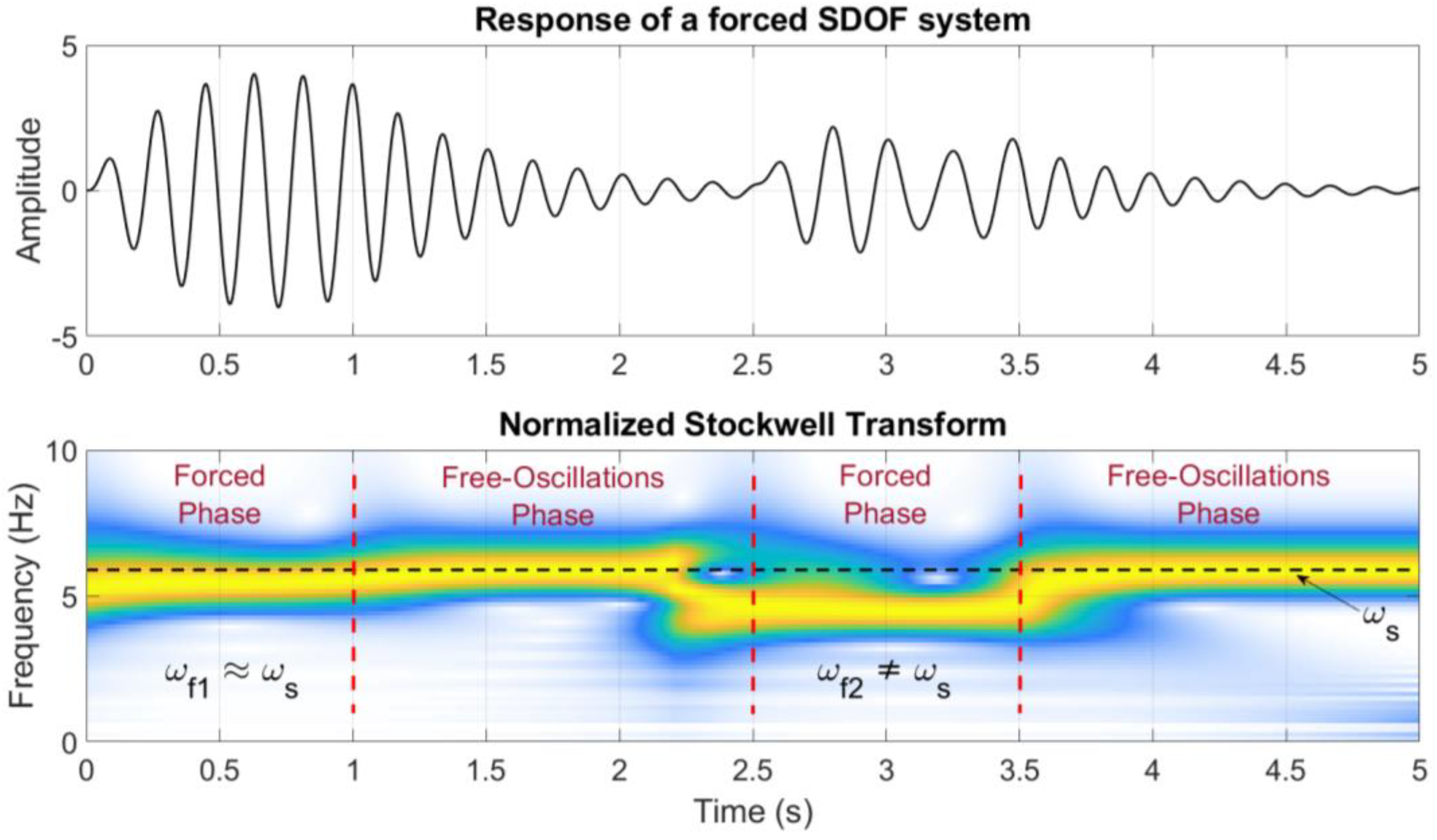
• Transient Response, corresponding to the solution of the associated homogenous solution, dependent on system characteristics and initial conditions (velocity and displacement).
• Steady-state Response, or regime, corresponding to the particular solution of the complete equation and dependant on the external force for which the maximum amplitude depends on the equivalent viscous damping factor and from the ratio between the frequency of the force $\left({\omega }_f\right)$ and the natural frequency of the system $\left({\omega }_0\right)$.

In contrast to the linear SDOF system, because of the nonlinear chaotic response, it is not possible to provide a general solution to estimate the settling time of the Duffing oscillator, since it is nonlinear and depends on the values assumed by the coefficients and initial conditions (Figure 5).

The concept of settling time is particularly important for understanding where the combination of input and forcing is such that it cannot be discriminated when acquisitions are made on a real system where the forcing is not perfectly known in all its components, i.e., always. In fact, whether it is a building or a bridge, the forcing is never perfectly known and can never be acquired. Consider the impact of wind or vibrations caused by internal forces within the system, such as vehicles passing over a bridge or vibrations caused by occupants inside a building. Therefore, there will almost always be some input of unknown origin that will generate a system response similar to that shown in Figure 1, where the transition from non-stationary to stationary could be mistaken for a modest frequency change. The situation may be further complicated by the fact that monitored systems are often subject to even slight variations in mass, stiffness, and damping. However, for low input values, they can cause fluctuations in the dynamic parameters of the system such that they lead to uncertainties in the estimation of eigenfrequencies and, consequently, in the definition of alarm thresholds. To this end, Equation (4) was defined in this paper to describe, in general, the considered SDOF system, in which the uncertainty parameters on mass estimation, damping, and stiffness were considered.

$$\left[m+{\epsilon }_m\left(t\right)\right]·\ddot{u}\left(t\right)+\left[c+{\epsilon }_c\left(t\right)\right]·\dot{u}\left(t\right)+[k+{\epsilon }_k\left(t\right)]·u\left(t\right)+\beta ·{u\left(t\right)}^3=f\left(t\right)$$

(4)

where m, c, k, and $\beta$ are constants, while ${\epsilon }_m\left(t\right)$, ${\epsilon }_c\left(t\right)$, and ${\epsilon }_k\left(t\right)$ are random variables characterizing small disturbances, and f$\left(t\right)$ represents the external excitation. As discussed earlier, since it is not possible to solve Equation (4) analytically, it was necessary to write a MATLAB^® [40] code (validated using the case histories for which the theoretical solution is available) to solve the nonlinear equation of motion and to perform Monte Carlo simulations [41,42].

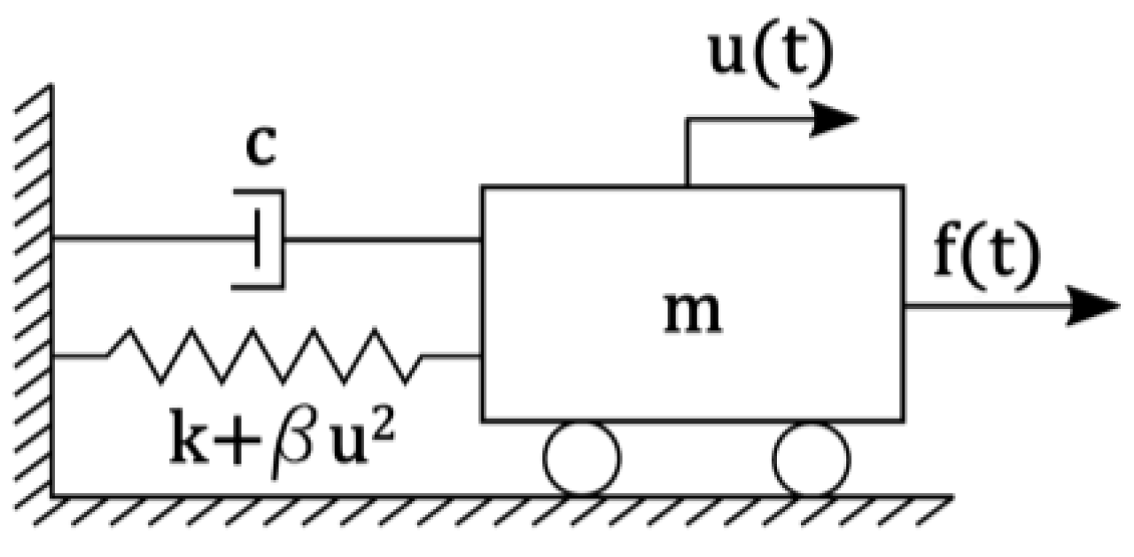
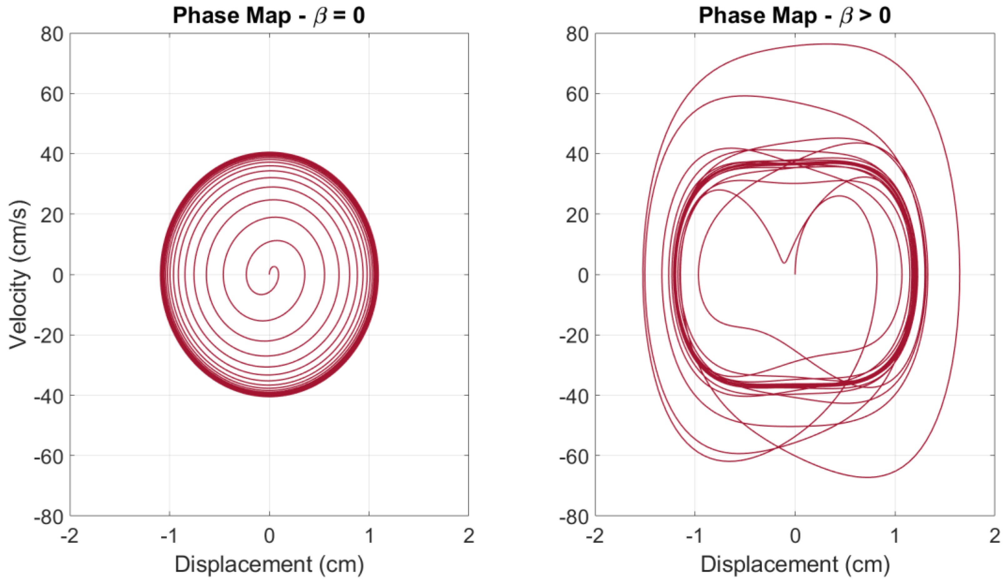
3. Numerical Model and Input Motion

In engineering applications, mechanical systems often exhibit nonlinear behaviour due to various factors such as geometric effects, operational conditions, excitations, and materials [43,44]. Therefore, it is appropriate to consider these nonlinear effects to achieve more accurate response predictions. Moreover, models aimed at representing mechanical systems are subject to uncertainties stemming from various sources, including variations in material parameters, boundary conditions, environmental factors, random excitations, and modelling assumptions, which should be considered to enhance the model’s predictability. The parametric approach inherently incorporates uncertainties stemming from two primary sources: random excitations and variability in design parameters. These uncertainties can be modelled either as fixed random variables or as dynamic stochastic processes that evolve over time. The response of nonlinear dynamical systems for stochastic inputs has been extensively studied in recent decades (see [38] and references therein). Generally, uncertain design parameters (such as masses, stiffness, and damping) are modelled as random variables, while stochastic excitations are often represented as stochastic processes, which can follow Gaussian or non-Gaussian distributions. While the Gaussian distribution is commonly used for its mathematical convenience and the similarity of many stochastic processes to its bell-shaped curve, stochastic processes are often constrained, calling into question the assumption of a Gaussian distribution. In the case of the Duffing oscillator, many studies have examined its response under stochastic excitations and/or random design parameters. Stochastic excitations have been modelled as Gaussian white noise, Poisson white noise, non-Gaussian stationary processes, and non-stationary processes. Additionally, some studies have separately considered random design parameters such as mass, stiffness, and damping. However, the literature currently lacks a comprehensive analysis comparing responses under different stochastic processes. Furthermore, clear thresholds are needed to distinguish whether changes in eigenfrequencies are caused by mechanical damage or other unrelated factors. To address this issue, we have developed numerical routines and functions to evaluate the response of the stochastic oscillator model (Equation (4)) to stochastic input motion. To simulate perturbations in the mass, damping, and stiffness parameters, as well as the beta parameter, we applied these methods (Figure 6). The numerical equation was solved for each simulation using Newmark numerical integration [45].

Drawing from the principles of complex systems physics, it is evident that deterministic forecasting of their long-term behaviour is not always possible. Instead, focusing on emergent properties can significantly enhance their analysis. Emergent properties are macroscopic characteristics that define the system and its behaviours. This research focuses on emergent properties, specifically targeting frequency variations that do not originate from substantial modifications in the system’s mechanical properties and are therefore unrelated to damage that would cause permanent changes in stiffness, mass, or damping qualities. To investigate this phenomenon, Monte Carlo simulations were executed using a system illustrated in Figure 7, which captures its key features. To reduce uncertainties in estimating the system’s natural frequency for each simulation, inputs with a duration of 1800 s were used. The study analysed three distinct oscillators with fundamental oscillation frequencies of 1 Hz, 5 Hz, and 10 Hz, respectively, using the inputs mentioned earlier. The equivalent viscous damping factor had a median value of 5%, and the beta values were parameterized, ranging from −1.5k to 1.5k, with k representing the median value of the system’s stiffness.

To supplement the analyses conducted with stochastic inputs, we examined the distributions of the two horizontal plane components of three actual earthquakes sourced from the ITACA database [46]. These earthquakes (

Table 1. Earthquakes selected for numerical simulations.

Event Name	Event Date	Magnitude W	Epicentral Distance (km)	Component	PGA (m/s2)
Central Italy	21 January 2017	3.7	3.7	E-W	−0.547
Central Italy	21 January 2017	3.7	3.7	N-S	−0.619
Central Italy	31 August 2016	3.5	4.5	E-W	0.753
Central Italy	31 August 2016	3.5	4.5	N-S	−0.504
Central Italy	23 April 2009	3.9	3.2	E-W	0.623
Central Italy	23 April 2009	3.9	3.2	N-S	−0.321

) are characterised by moderate accelerations, which are not strong enough to cause significant structural nonlinearities in the investigated system. We considered the following accelerometer traces.

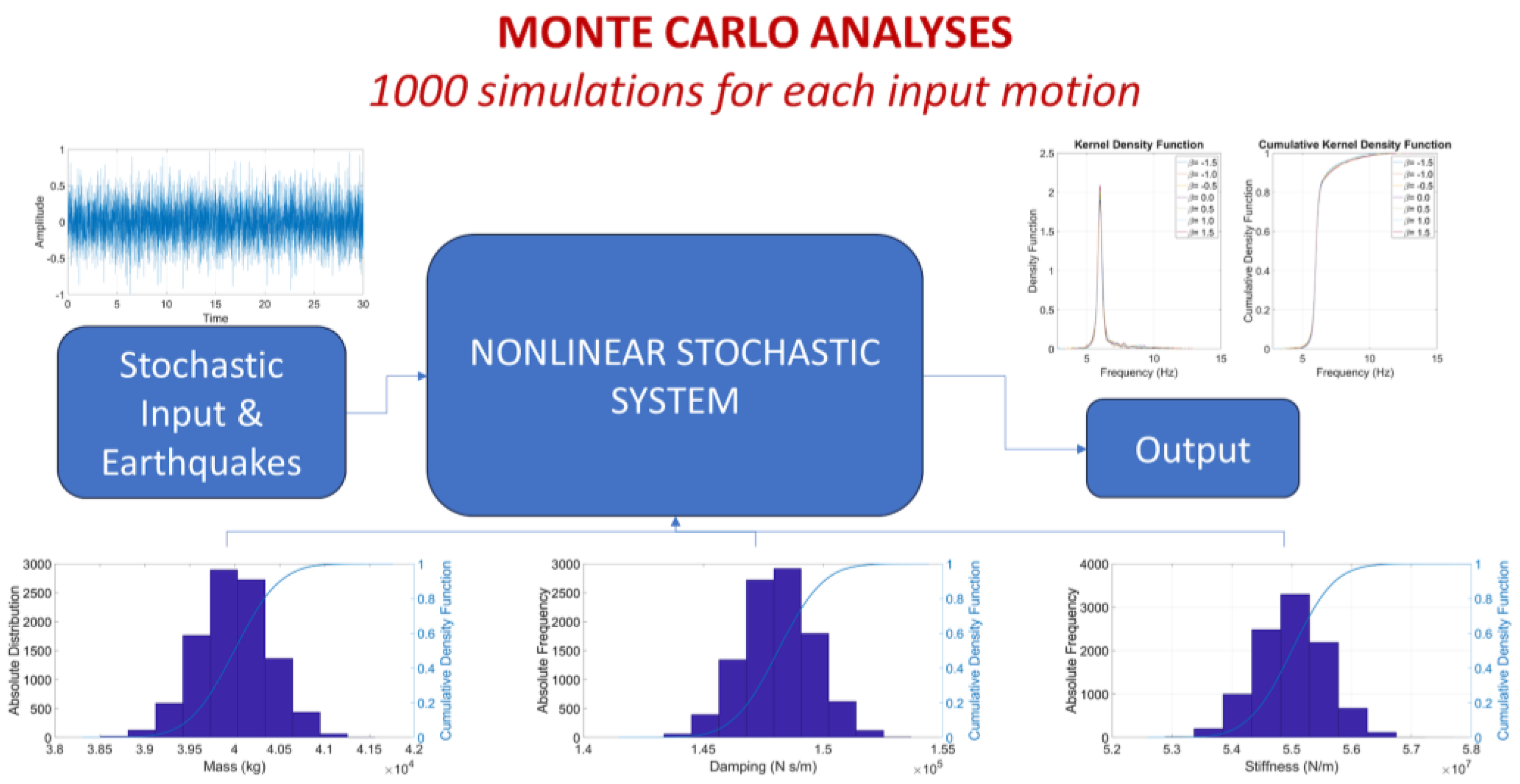
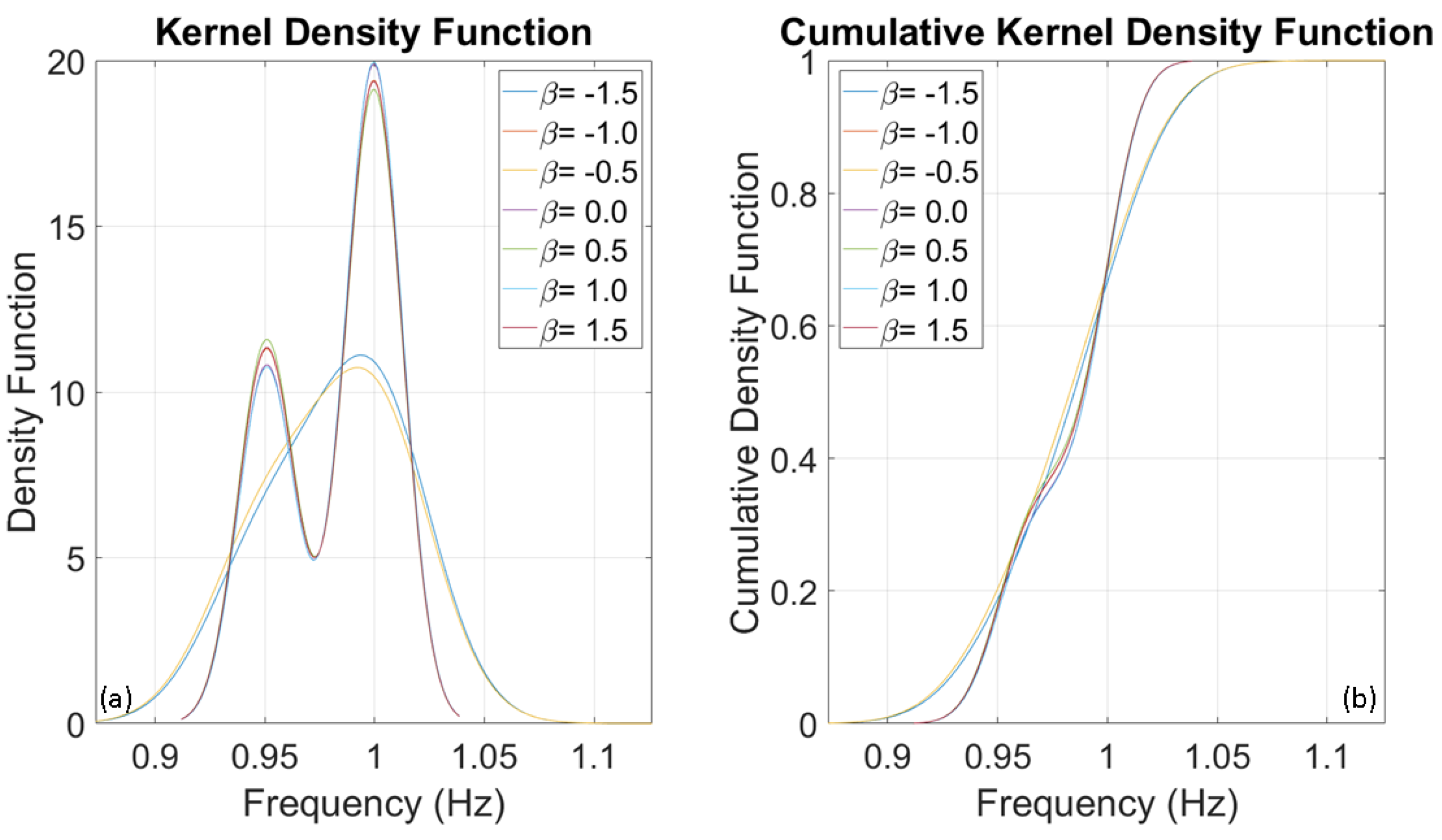
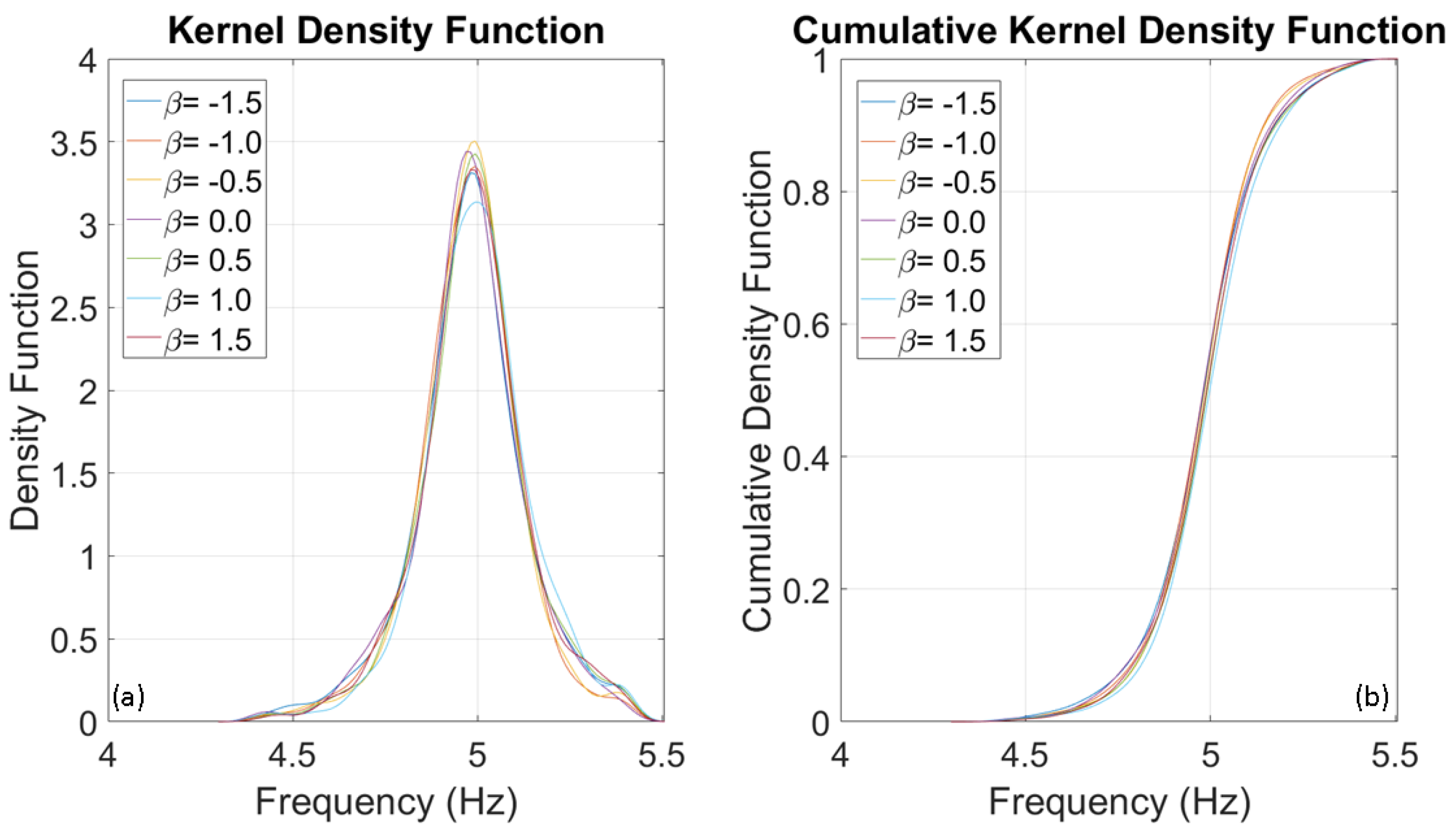
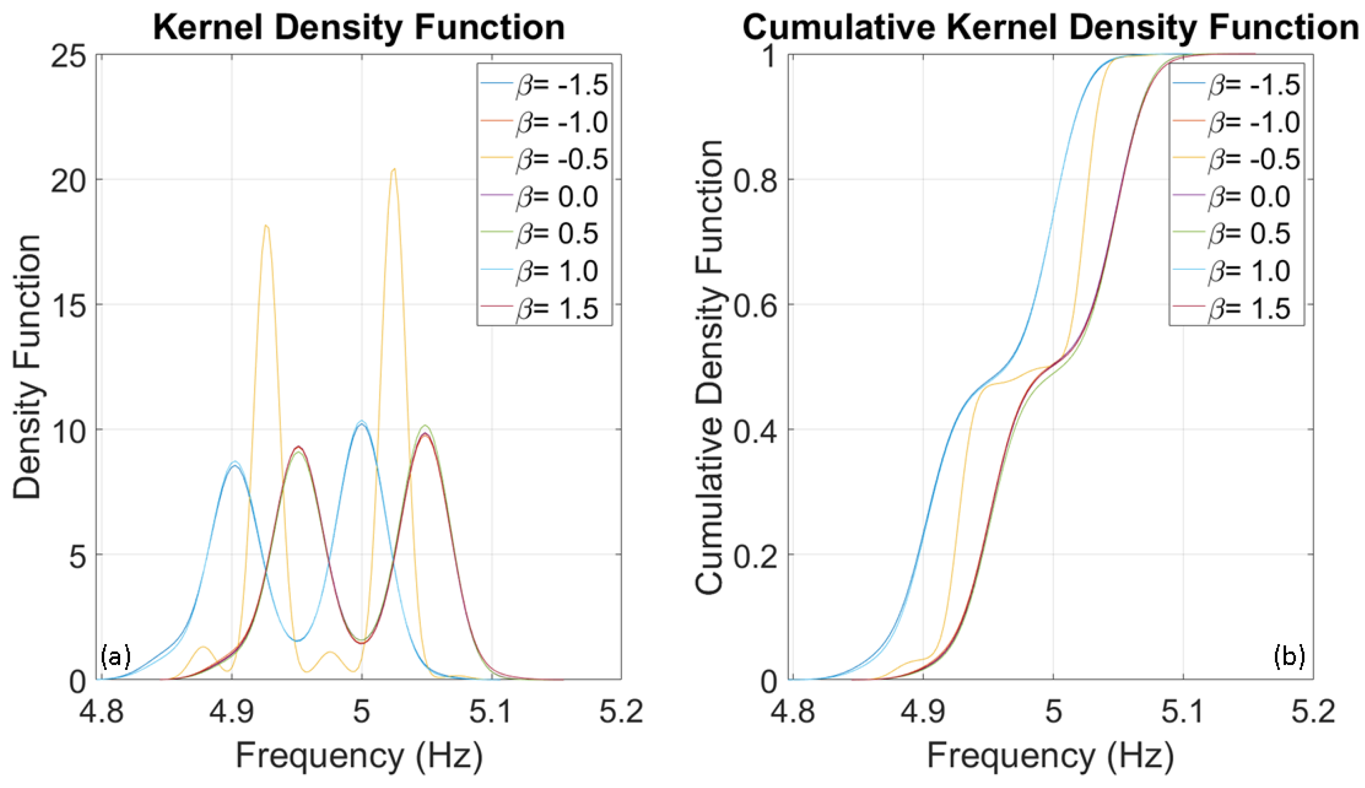
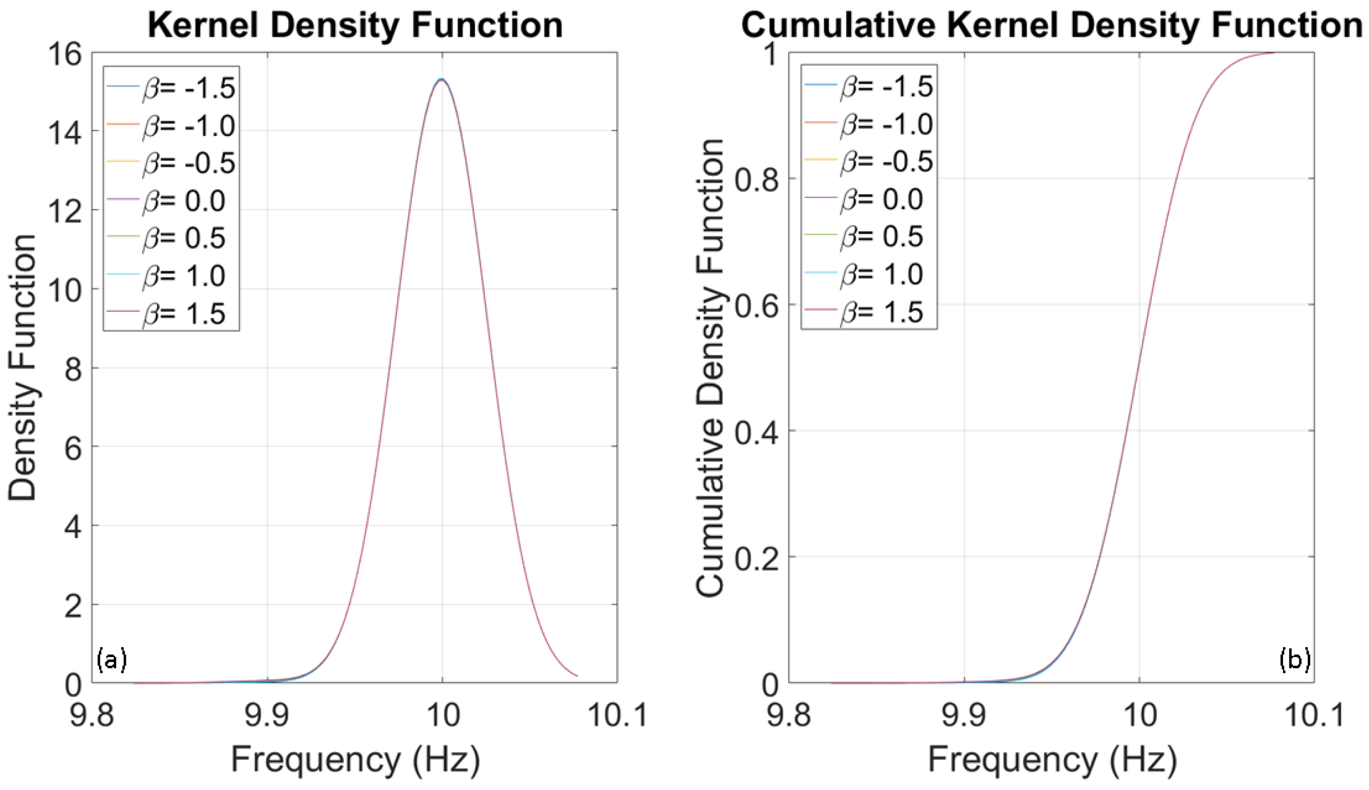
4. Results of Monte Carlo Simulations

As explained earlier, we conducted Monte Carlo simulations using MATLAB^® codes and functions to evaluate how the specified parameters affect the dynamic response of the Single-Degree-of-Freedom (SDOF) system. Our objective was to establish thresholds for detecting changes in the fundamental frequency caused by non-stationary responses. These variations are caused by the interaction between the input and system response, which is influenced by minor nonlinearities resulting from the interaction between primary and secondary elements.

To evaluate the frequencies of three SDOF systems with fundamental frequencies of 1, 5, and 10 Hz, several thousand numerical simulations were conducted using stochastic input motions. The number of simulations for each oscillator was adjusted until the outcomes reached a stable state, identified at 1000 simulations. The probability distributions of the evaluated frequencies for the three oscillators are presented below. Upon analysing Figure 8, Figure 9 and Figure 10, it is clear that the dispersion of the results increases as the fundamental frequency of the analysed oscillator increases. The dispersion of the estimated frequencies appears to be minimally dependent on Duffing’s beta parameter. However, in some cases, the shape of the distribution is noticeably influenced by it. In this oscillation regime, the beta parameter acts as a disturbance on the structural response in terms of amplitude and waveform, but not in terms of frequency variation. This disturbance is similar to those caused by interactions between structural and non-structural components, constraints, friction, and other factors.

Robust estimators were used to define thresholds for the 1 Hz and 10 Hz Single-Degree-of-Freedom (SDOF) systems due to their non-normal statistical distribution. This required evaluating median and percentile parameters. Figure 11 shows the frequency variations for each SDOF system associated with the 5th, 25th, 75th, and 95th percentiles. It is important to note that the results were parameterized based solely on the fundamental frequency of the SDOF, treating all variable parameters as noise. The curve representing the median value calculated for each percentile is also included, providing a comprehensive visualization of the frequency variation across the different percentiles.

Table 2. Percentiles of frequency variations evaluated from results of Monte Carlo Simulations.

	5th Percentage	25th Percentage	75th Percentage	95th Percentage
1 Hz System	−2.3%	−2.3%	2.5%	2.5%
5 Hz System	−4.9%	−1.9%	1.0%	4.9%
10 Hz System	−11.2%	−2.9%	1.0%	2.9%
MEAN	−6.1%	−2.4%	1.5%	3.4%

presents the statistical values for frequency variation, evaluated in relation to the nominal fundamental frequency of each system. Percentiles were evaluated by considering a vector named A composed of n-elements, the sorted elements in A are taken as the 100(0.5/n)^th, 100(1.5/n)^th,..., 100([n − 0.5]/n)^th percentiles (see MATLAB^® [40]).

Moreover, Table 2 presents mean values proposed as thresholds for frequency variations associated with the non-stationary linear dynamic behaviour of structures under operational conditions. Figure 10 displays the alignment of mean values, demonstrating the feasibility of using linear numerical regression to establish an empirical formulation. This formula enables the determination of the frequency limit for each percentile, providing a systematic approach to quantify the threshold for frequency variations in structural dynamics.

$$\Delta F_{LIM}(\%)=0.1\ast x-5.9$$

(5)

where $\Delta F_{LIM}$ represents the limit of the frequency variation expressed as a percentage, and x represents the reference percentile. With respect to the data, the regression formula exhibits a correlation index of R² = 0.97. In general, considering that the structural damage induced by critical events generates a negative stiffness variation (in the sense that the stiffness of the damaged system is less than the stiffness of the undamaged system), small positive frequency variations cause fewer problems and are more easily associated with phenomena other than structural damage.

Small negative variations can more easily be confused with the presence of structural damage. Therefore, from the perspective of alert systems, average negative variations can be considered as damage thresholds at different probability levels. An average variation of −6.1% (5th percentile indicated in Table 2) can be defined as a threshold value beyond which there is a 95% probability that the system may have suffered real damage, while an average variation of −2.4% (75th percentile indicated in Table 2) can be defined as a threshold value beyond which there is a 75% probability that the system may have suffered real damage. On the other hand, exceeding the thresholds of +1.5% and +3.4% for positive fast frequency variations could result in a 75% and 95% probability, respectively, of mass reduction, unlikely without damage, or SHM system malfunction. To evaluate the robustness of the proposed thresholds, further analyses were carried out by increasing the variability of damping and stiffness by 20% and 10%, respectively. The results showed that the proposed thresholds remained stable.

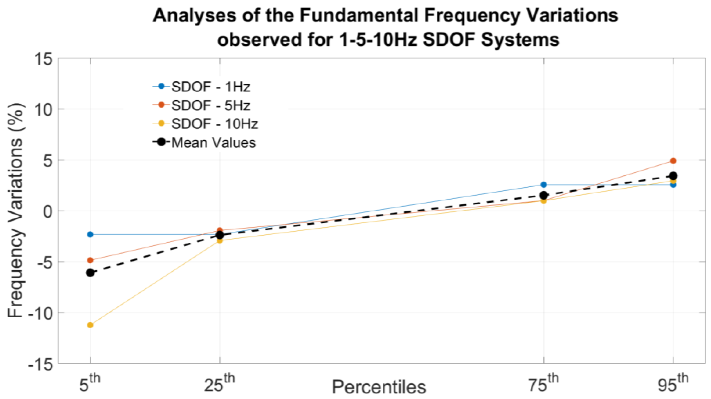
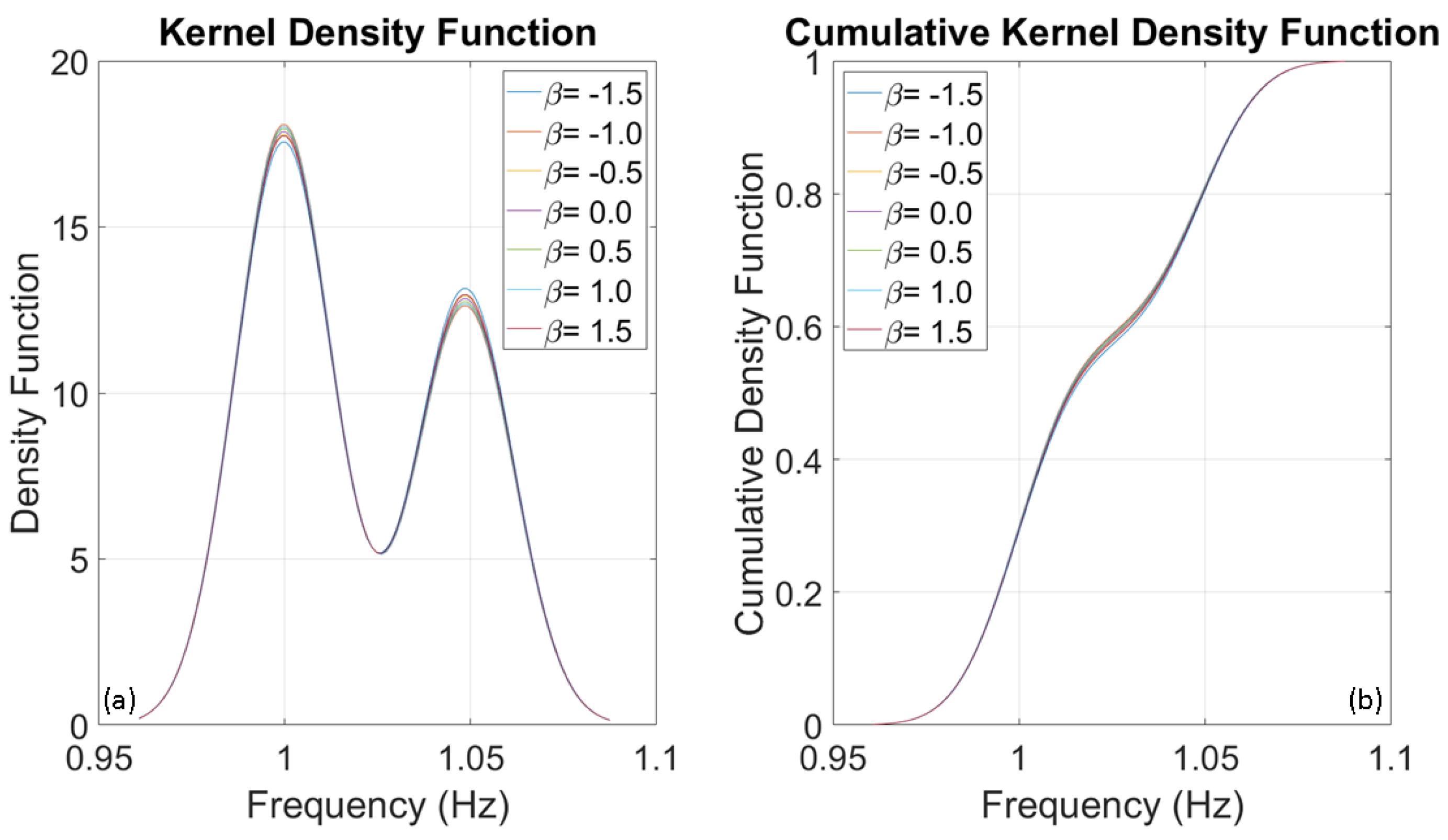
Analyses of Monte Carlo Simulations Carried Out Using Real Earthquakes

This section analyses the results of the Monte Carlo simulation using the selected earthquakes described in Section 3. Figure 12, Figure 13 and Figure 14 depict the Kernel Density Functions and Cumulative Distribution Functions related to the estimated fundamental frequencies of 1, 5, and 10 Hz SDOF systems.

The Duffing coefficient was parameterised in the numerical simulations within the accelerometric record of each earthquake. Gaussian noise was also introduced in the mass, damping, and stiffness, with a maximum noise value of 1%. The statistical distributions of frequency measurements obtained from the numerical simulations are presented below, similar to the previous section. The statistical values of the frequency variation are evaluated with respect to the nominal fundamental frequency of each system (

Table 3. Percentiles of frequency variations evaluated from results of Monte Carlo Simulations using the selected real earthquakes.

	5th Percentage	25th Percentage	75th Percentage	95th Percentage
1 Hz System	−2.3%	−2.3%	2.5%	2.5%
5 Hz System	−1.0%	−1.0%	1.0%	1.0%
10 Hz System	−0.0%	−0.0%	0.8%	0.8%
MEAN	−1.1%	−1.1%	1.4%	1.4%

).

The fundamental frequency variations determined by real earthquakes confirmed the limits established in the previous section using stochastic input motion. It is unlikely that real signals will exceed these limits as they typically lack the frequency content of stochastic signals.

5. Discussion and Conclusions

Structural systems can deteriorate over time due to aging or be severely impacted by sudden catastrophic events, such as earthquakes, explosions, and hurricanes. Therefore, structural health monitoring is crucial for early identification of damage to prevent disastrous outcomes.

The manuscript delves into the study of chaotic effects on real systems induced by factors that cannot be precisely quantified, such as the influence of non-structural components, non-stationary effects arising from the superposition of input and response, and random variations in mass, stiffness, and damping, among others. Given the nonlinear nature of the problem and the significant presence of stochastic variables, an analytical solution is unfeasible. Therefore, numerical and statistical methods were employed to explore this complex phenomenon. This investigation culminated in the identification of behavioural thresholds applicable in automated damage assessment systems, which were correlated with frequency variations in the monitored system.

To tackle this challenge, the study conducted extensive Monte Carlo simulations using Single-Degree-of-Freedom (SDOF) systems that represent the individual vibrational modes of Multi-Degree-of-Freedom (MDOF) systems. The simulations modelled realistic structural entities and subjected them to various inputs. Parameters such as mass, damping, and stiffness were accurately simulated. The models’ equations were solved using the Newmark algorithm, which distinguishes between non-stationary effects and actual structural damage. Statistical analysis was crucial in determining threshold values for damage detection. Non-stationary linear variations were identified within a range of −6.1% to +3.4%. These thresholds reduce the risk of false positives. The established thresholds for quantifying frequency variations in Single-Degree-of-Freedom (SDOF) systems during real earthquakes were confirmed by additional simulations. This enhances the reliability of structural health assessments. As a result, the probability of false alarms in structural health monitoring systems will be reduced. A simplified scheme of the introduction of thresholds within a monitoring system is depicted in Figure 15.

Future studies could benefit greatly from incorporating experimental data obtained from continuously monitored structures and specimens. These data should include a comprehensive evaluation of the influence of both structural and non-structural elements, such as bearings and infills, and should cover a range of vibrations, including ambient and event-induced vibrations, to support numerical findings. Additional research is needed to discern the differences and similarities among MDOF systems.

References

1. Sun, X.; Ilanko, S.; Mochida, Y.; Tighe, R.C. A Review on Vibration-Based Damage Detection Methods for Civil Structures. Vibration 2023, 6, 843–875. [Google Scholar] [CrossRef]
2. Hellier, C. Handbook of Nondestructive Evaluation, 2nd ed.; McGraw Hill Professional: New York, NY, USA, 2013. [Google Scholar]
3. Avci, O.; Abdeljaber, O.; Kiranyaz, S.; Hussein, M.; Gabbouj, M.; Inman, D.J. A review of vibration-based damage detection in civil structures: From traditional methods to Machine Learning and Deep Learning applications. Mech. Syst. Signal Proc. 2021, 147, 107077. [Google Scholar] [CrossRef]
4. Wang, Z.; Ong, K. Autoregressive coefficients based Hotelling’s T2 control chart for structural health monitoring. Comput. Struct. 2008, 86, 1918–1935. [Google Scholar] [CrossRef]
5. Teughels, A.; Maeck, J.; De Roeck, G. Damage assessment by FE model updating using damage functions. Comput. Struct. 2002, 80, 1869–1879. [Google Scholar] [CrossRef]
6. Rytter, A. Vibrational Based Inspection of Civil Engineering Structures. Ph.D. Thesis, Department of Building Technology and Structural Engineering, Aalborg University, Aalborg, Denmark, 1993. [Google Scholar]
7. Caddemi, S.; Calio, I.; Cannizzaro, F.; Morassi, A. A procedure for the identification of multiple cracks on beams and frames by static measurements. Struct. Control Health Monit. 2018, 25, e2194. [Google Scholar] [CrossRef]
8. Buda, G.; Caddemi, S. Identification of concentrated damages in Euler-Bernoulli beams under static loads. J. Eng. Mech. 2007, 133, 942–956. [Google Scholar] [CrossRef]
9. Doebling, S.W.; Farrar, C.R.; Prime, M.B. A summary review of vibration-based damage identification methods. Shock. Vib. Dig. 1998, 30, 91–105. [Google Scholar] [CrossRef]
10. Sekhar, A.S. Multiple cracks effects and identification. Mech. Syst. Signal Proc. 2008, 22, 845–878. [Google Scholar] [CrossRef]
11. Limongelli, M.P.; Siegert, D.; Merliot, E.; Waeytens, J.; Bourquin, F.; Vidal, R.; Le Corvec, V.; Gueguen, I.; Cottineau, L.M. Damage detection in a post tensioned concrete beam—Experimental investigation. Eng. Struct. 2016, 128, 15–25. [Google Scholar] [CrossRef]
12. Bonopera, M. Stress Evaluation in Axially Loaded Members of Masonry Buildings and Space Structures: From Traditional Methods to Combinations with Artificial Intelligence Approaches. Buildings 2023, 13, 2097. [Google Scholar] [CrossRef]
13. Fan, W.; Qiao, P. Vibration-based damage identification methods: A review and comparative study. Struct. Health Monit. 2011, 10, 83–111. [Google Scholar] [CrossRef]
14. Katunin, A. Nondestructive damage assessment of composite structures based on wavelet analysis of modal curvatures: State-of-the-art review and description of wavelet-based damage assessment benchmark. Shock Vib. 2015, 2015, 735219. [Google Scholar] [CrossRef]
15. Ditommaso, R.; Mucciarelli, M.; Ponzo, F.C. Analysis of non-stationary structural systems by using a band-variable filter. Bull. Earthq. Eng. 2012, 10, 895–911. [Google Scholar] [CrossRef]
16. Stockwell, R.G.; Mansinha, L.; Lowe, R.P. Localization of the complex spectrum: The S-transform. IEEE Trans. Signal Process 1996, 44, 998–1001. [Google Scholar] [CrossRef]
17. Ditommaso, R.; Ponzo, F.C. Automatic evaluation of the fundamental frequency variations and related damping factor of reinforced concrete framed structures using the Short Time Impulse Response Function (STIRF). Eng. Struct. 2015, 82, 104–112. [Google Scholar] [CrossRef]
18. Ditommaso, R.; Ponzo, F.C.; Auletta, G. Damage detection on framed structures: Modal curvature evaluation using Stockwell Transform under seismic excitation. Earthq. Eng. Eng. Vib. 2015, 14, 265–274. [Google Scholar] [CrossRef]
19. Iacovino, C.; Ditommaso, R.; Ponzo, F.; Limongelli, M. The Interpolation Evolution Method for damage localization in structures under seismic excitation. Earthq. Eng. Struct. Dyn. 2018, 47, 2117–2136. [Google Scholar] [CrossRef]
20. Ditommaso, R.; Iacovino, C.; Auletta, G.; Parolai, S.; Ponzo, F.C. Damage detection and localization on real structures subjected to strong motion earthquakes using the curvature evolution method: The Navelli (Italy) case Study. Appl. Sci. 2021, 11, 6496. [Google Scholar] [CrossRef]
21. Cataldo, A.; Roselli, I.; Fioriti, V.; Saitta, F.; Colucci, A.; Tatì, A.; Ponzo, F.C.; Ditommaso, R.; Mennuti, C.; Marzani, A. Advanced Video-Based Processing for Low-Cost Damage Assessment of Buildings under Seismic Loading in Shaking Table Tests. Sensors 2023, 23, 5303. [Google Scholar] [CrossRef]
22. Bovsunovsky, A.; Surace, C. Non-linearities in the vibrations of elastic structures with a closing crack: A state of the art review. Mech. Syst. Signal Proc. 2015, 62–63, 129–148. [Google Scholar] [CrossRef]
23. Giannini, O.; Casini, P.; Vestroni, F. Nonlinear harmonic identification of breathing cracks in beams. Comput. Struct. 2013, 129, 166–177. [Google Scholar] [CrossRef]
24. Caddemi, S.; Caliò, I.; Marletta, M. The dynamic non-linear behaviour of beams with closing cracks. In Proceedings of the AIMETA 2009 XIX Congresso di Meccanica Teorica ed Applicata, Ancona, Italy, 14–17 September 2009. [Google Scholar]
25. Kisa, M.; Brandon, J. The effects of closure of cracks on the dynamics of a cracked cantilever beam. J. Sound Vibr. 2000, 238, 1–18. [Google Scholar] [CrossRef]
26. Deng, Z.; Huang, M.; Wan, N.; Zhang, J. The Current Development of Structural Health Monitoring for Bridges: A Review. Buildings 2023, 13, 1360. [Google Scholar] [CrossRef]
27. Luo, J.; Huang, M.; Lei, Y. Temperature Effect on Vibration Properties and Vibration-Based Damage Identification of Bridge Structures: A Literature Review. Buildings 2022, 12, 1209. [Google Scholar] [CrossRef]
28. Liu, C.; DeWolf, J.T. Effect of temperature on modal variability of a curved concrete bridge under ambient loads. J. Struct. Eng. 2007, 133, 1742–1751. [Google Scholar] [CrossRef]
29. Xia, Y.; Hao, H.; Zanardo, G.; Deeks, A. Long term vibration monitoring of an RC slab: Temperature and humidity effect. Eng. Struct. 2006, 28, 441–452. [Google Scholar] [CrossRef]
30. Sohn, H. Effects of environmental and operational variability on structural health monitoring. Philos. Trans. A Math. Phys. Eng. Sci. 2007, 365, 539–560. [Google Scholar] [CrossRef]
31. Peeters, B.; De Roeck, G. One-year monitoring of the Z24-Bridge: Environmental effects versus damage events. Earthq. Eng. Struct. Dyn. 2001, 30, 149–171. [Google Scholar] [CrossRef]
32. Limongelli, M.P. Frequency response function interpolation for damage detection under changing environment. Mech. Syst. Signal Process. 2010, 24, 2898–2913. [Google Scholar] [CrossRef]
33. Karakostas, C.; Quaranta, G.; Chatzi, E.; Zülfikar, A.C.; Çetindemir, O.; De Roeck, G.; Döhler, M.; Limongelli, M.P.; Lombaert, G.; Apaydın, N.M.; et al. Seismic assessment of bridges through structural health monitoring: A state-of-the-art review. Bull. Earthq. Eng. 2023, 22, 1309–1357. [Google Scholar] [CrossRef] [PubMed]
34. Ponzo, F.C.; Auletta, G.; Ielpo, P.; Ditommaso, R. DInSAR–SBAS satellite monitoring of infrastructures: How temperature affects the “Ponte della Musica” case study. J. Civ. Struct. Health Monit. 2024. [Google Scholar] [CrossRef]
35. Mucciarelli, M.; Gallipoli, M.R. Non-parametric analysis of a single seismometric recording to obtain building dynamic parameters. Ann. Geophys. 2007. [Google Scholar] [CrossRef]
36. Duffing, G. Erzwungene Schwingungen bei veränderlicher Eigenfrequenz und ihre Technische Bedeutung; [Forced oscillations with variable natural frequency and their technical relevance]; Vieweg: Braunschweig, Germany, 1918; Volume Heft 41/42, p. vi+134, OCLC 12003652. (In German) [Google Scholar]
37. Gabos, Z.; Barton, D.A.W.; Dombovari, Z. Equation-free bifurcation analysis of a stochastically excited Duffing oscillator. J. Sound Vib. 2023, 547, 117536. [Google Scholar] [CrossRef]
38. Lobo, D.M.; Ritto, T.G.; Castello, D.A.; Cataldo, E. Dynamics of a Duffing oscillator with the stiffness modeled as a stochastic process. Int. J. Non-Linear Mech. 2019, 116, 273–280. [Google Scholar] [CrossRef]
39. Cui, J.; Jiang, W.A.; Xia, Z.W.; Chen, L.Q. Non-stationary response of variable-mass Duffing oscillator with mass disturbance modeled as Gaussian white noise. Physica A 2019, 526, 121018. [Google Scholar] [CrossRef]
40. MATLAB R2023b Software 1994–2024; The MathWorks, Inc.: Natick, MA, USA, 2023.
41. Kevin, P. MacKeown Stochastic Simulation in Physics; Springer: Berlin/Heidelberg, Germany, 1997; ISBN 981-3083-26-3. [Google Scholar]
42. Bernd, A. Berg Markov Chain Monte Carlo Simulations and Their Statistical Analysis (with Web-Based Fortran Code); World Scientific: Singapore, 2004; ISBN 981-238-935-0. [Google Scholar]
43. Villani, L.G.G.; Da Silva, S.; Cunha, A., Jr. Identification of a nonlinear beam through a stochastic model based on a duffing oscillator. In Proceedings of the 6th International Conference on Nonlinear Science and Complexity, São José dos Campos, Brazil, 16–20 May 2017. [Google Scholar] [CrossRef]
44. Villani, L.G.; Silva, S.D.; Cunha, A. Application of a stochastic version of the restoring force surface method to identify a Duffing oscillator. In Proceedings of the First International Nonlinear Dynamics Conference, NODYCON 2019, Rome, Italy, 17–20 February 2019; pp. 1–3. [Google Scholar]
45. Newmark, N.M. A method of computation for structural dynamics. J. Eng. Mech. Div. 1959, 85, 67–94. [Google Scholar] [CrossRef]
46. Felicetta, C.; Russo, E.; D’Amico, M.; Sgobba, S.; Lanzano, G.; Mascandola, C.; Pacor, F.; Luzi, L. Italian Accelerometric Archive v4.0—Istituto Nazionale di Geofisica e Vulcanologia, Dipartimento della Protezione Civile Nazionale. 2023. Available online: https://itaca.mi.ingv.it/ItacaNet_40/#/home (accessed on 27 February 2024).
Figure 1. Example of fundamental frequency variations evaluated with the Stockwell transform on an accelerometer recording (vertical component) acquired on the “Ponte della Musica—Armando Trovajoli” bridge.
Buildings 14 00821 g001
Figure 2. Graphic representation of the structural response of an SDOF system characterized by an equivalent viscous damping factor and fundamental frequency equal to 5% and 5.89 Hz, respectively, and forced by an 18 Hz sinusoid.
Buildings 14 00821 g002
Figure 3. Example of apparent variations in eigenfrequency retrieved during the transition phases of a linear Single-Degree-of-Freedom (SDOF) system. The system is characterized by a fundamental frequency of 5.89 Hz and was forced at two different times with two different input frequencies, wf1 and wf2.
Buildings 14 00821 g003
Figure 4. General representation of the Duffing oscillator.
Buildings 14 00821 g004
Figure 5. Qualitative example of Phase Maps evaluated for two Single-Degree-of-Freedom (SDOF) systems subjected to the same forcing. The left side shows a stationary behaviour, while the right side shows the dynamic response of an SDOF system, which, with an appropriate combination of Duffing coefficient, intensity, and frequency of the forcing, can exhibit a chaotic behaviour.
Buildings 14 00821 g005
Figure 6. Simplified scheme of the stochastic process implemented to analyse the response of the nonlinear SDOF system.
Buildings 14 00821 g006
Figure 7. Simplified scheme of the stochastic process implemented for Monte Carlo simulations.
Buildings 14 00821 g007
Figure 8. (a) Kernel Density Function and (b) Cumulative Distribution Function of 1 Hz SDOF system retrieved from Monte Carlo simulations.
Buildings 14 00821 g008
Figure 9. (a) Kernel Density Function and (b) Cumulative Distribution Function of 5 Hz SDOF system retrieved from Monte Carlo simulations.
Buildings 14 00821 g009
Figure 10. (a) Kernel Density Function and (b) Cumulative Distribution Function of 10 Hz SDOF system retrieved from Monte Carlo simulations.
Buildings 14 00821 g010
Figure 11. Evaluation of characteristic values of frequency variation for the 5th, 25th, 75th, and 95th percentiles.
Buildings 14 00821 g011
Figure 12. (a) Kernel Density Function and (b) Cumulative Distribution Function of 1 Hz SDOF system retrieved from Monte Carlo simulations using earthquakes.
Buildings 14 00821 g012
Figure 13. (a) Kernel Density Function and (b) Cumulative Distribution Function of 5 Hz SDOF system retrieved from Monte Carlo simulations with real earthquakes.
Buildings 14 00821 g013
Figure 14. (a) Kernel Density Function and (b) Cumulative Distribution Function of 10 Hz SDOF system retrieved from Monte Carlo simulations with real earthquakes.
Buildings 14 00821 g014
Figure 15. Simplified scheme related to the introduction of thresholds to minimize false alarms within the algorithm of an SHM system based on eigenfrequencies variations.
Buildings 14 00821 g015