Reliability-Centric Maintenance Planning for Bridge Infrastructure: A Novel Method Based on Improved Electric Fish Optimization

Abstract

Bridge infrastructure provides an important effect on contemporary transportation networks, and its upkeep is significant for ensuring public safety and reducing economic impacts. Nevertheless, the aging and degradation of bridge structures present considerable challenges for asset managers, who must navigate the necessity of maintenance against constrained financial resources. Conventional maintenance approaches typically emphasize reactive repairs, which can result in elevated lifecycle expenses and risk structural integrity. This paper introduces an innovative framework aimed at optimizing bridge maintenance expenditures while maintaining structural safety. The proposed methodology incorporates a reliability-based deterioration model, an intervention effect model, a financial model, and an optimization model empowered by an Improved Electric Fish Optimization (IEFO) algorithm. The framework is demonstrated through a case study of a reinforced bridge framework designed according to the standards of Canadian highway bridge design. The findings illustrate that the proposed methodology can substantially lower lifecycle costs by investigating the most economical maintenance strategies, including minor repairs that can postpone the necessity for expensive major interventions. The optimal scenario identified by the IEFO algorithm yielded lower equivalent uniform annual costs in comparison with the traditional scenario focused solely on major repairs. This research advances the field of data-driven maintenance planning for bridge infrastructure, empowering asset managers to make well-informed decisions that effectively balance cost and safety considerations.

1. Introduction

Bridges are one of the basic components of highways in all countries, and their construction costs are usually higher than other road infrastructures [1]. Deterioration of bridges, along with increased traffic load, extreme environmental conditions, and their specific locations, leads to a rapid decrease in the integrity of their structural elements, which requires urgent maintenance efforts [2]. Like all structures, bridges are significantly affected by environmental factors, and despite proper design and implementation, various elements affect their lifespans and conditions. Due to their high cost and sensitivity, maintenance is often inadequate [3].

In this scenario, it will have detrimental effects. Consequently, regular inspections are essential to prevent incurring excessive costs associated with rectifying these damages. As a result, many policies regarding the management and oversight of bridges worldwide acknowledge the necessity of routine inspections and maintenance throughout their operational lifespan [4].

However, there is a pressing need for planning in decision-making and design based on fundamental principles of durability and sustainability. There is a lack of understanding on how to ensure the long-term integrity of bridges. In specific instances, during the operational phase, there has been negligence in the maintenance of bridges, leading to a reliance on remedial strategies rather than proactive measures.

The bridge’s maintenance presents significant challenges, as the inevitable wear and tear of these structures occur over time [5]. Different factors contribute to the degradation of bridges, such as design choices, construction standards, material selection, the impact of natural disasters, and environmental influences. Historically, the use of less expensive materials has often resulted in increased maintenance expenses later on, as demonstrated by the eventual failure of wooden bridges [6]. In contemporary construction, bridges are made from a range of materials, including cast iron, concrete, steel, and both reinforced and pre-stressed concrete, each possessing distinct benefits and drawbacks [7].

As the number of bridges requiring specialized care continues to rise, the direct costs associated with engineering efforts become increasingly substantial. It is imperative to engage in rational decision-making to allocate financial resources effectively, particularly in light of the continuous loads and external factors that bridges are subjected to [8]. Ensuring proper maintenance is critical for the safety and longevity of these structures, which consistently contend with the forces of nature and the effects of time.

Ghodoosi et al. [9] aimed to establish a technique to forecast the most economical program for bridges while the safety of the structures is maintained within the least probable cost. The current technique has been employed in superstructure bridges that have been built according to the design standards of Canadian highway bridges. It was revealed by the findings that declining the quantity of overpriced main interventions and employing less expensive main repairs could decrease costs, which resulted in USD 8277, as a yearly cost. This number illustrated that this method was 4.5 times more economical compared with other traditional approaches. This unique technique was the integration of nonlinear finite-component modeling, genetic algorithm optimization, and reliability analysis.

Yao et al. [10] invented an approach based on DRL (Deep Reinforcement Learning) to have superior maintenance techniques with the purpose of maximizing a longstanding economical approach. The single-lane pavement segmentation could own various methods; moreover, the main aim of this optimization study was to have longstanding cost-effectiveness. The number of 42 variables embodied all the states. The variables were traffic loads, pavement materials and structures, pavement conditions, maintenance records, and so on. To do so, two expressways, Zhenli and Ningchang, were chosen. It was illustrated that the suggested model could somewhat enhance the cost-effectiveness of maintenance.

Wei et al. [11] suggested an automatic DRL model to achieve optimal structural maintenance. A DNN (Deep Neural Network) was utilized in the present study to achieve the state-action Q value based on historical data or simulation. Furthermore, the policy was accomplished by employing the Q value. The learning procedure’s optimization was based on a sample, so it could learn from actual historical data gathered from several bridges. A thorough approach was employed for various tasks of structure maintenance with very little alteration in the framework of the neural network. Several case studies with long-span cable-stayed bridges and 7 elements with 263 elements were implemented to display the suggested process. As was depicted by the outcomes, the suggested method could find an optimum policy for the task of maintaining complex and simple structures.

Wang et al. [12] developed an instance database of maintenance cost in the present research following actual data relevant to engineering and a forecast model of bridge maintenance expense established by employing a CNN (Convolutional Neural Network) and an ANN (Artificial Neural Network), respectively. Initially, eight major elements that influenced the costs of maintenance were assessed based on the stochastic forest approach, and then the findings of the assessment were certified employing exploratory data examination. After that, the original data were monitored based on isolation forest standards, and the GPD (Gross Domestic Product) rate of growth was employed to display the association between the maintenance costs of the bridge and the growth of the economy. The forecast efficacy of the CNN was superior to the fully connected ANN.

Yessoufou and Zhu [13] conducted a study and introduced a two-phase CNN–LSTM for damage identification of bridges by employing data of vibration while taking into account the effect of temperatures. Initially, a CNN–LSTM on the basis of categorization was designed to implement multiclass diagnosis tasks of damage. Then, a CNN–LSTM on the basis of regression was established for tasks of severity forecast and damage localization. The efficacy of the suggested approach for damage recognition was assessed by a simulation dataset of a concrete bridge highway and a Z24 bridge dataset in Switzerland. Furthermore, several assessment metrics were employed in the present study, which showed the superiority of the CNN–LSTM in comparison with traditional ML optimizers and normal CNNs for the damage recognition of bridges.

These occurrences underscore the necessity of proactive maintenance and management of bridges to safeguard public safety and reduce economic losses.

This study aims to contribute to the development of bridge maintenance optimization frameworks by proposing an innovative approach that integrates reliability-based deterioration modeling, financial modeling, intervention effect modeling, and optimization using an Improved Electric Fish Optimization (IEFO) algorithm. The proposed approach is employed in a case study of a simply supported bridge superstructure constructed based on Canadian highway bridge design standards. The results of this study demonstrate the effectiveness of the proposed approach in minimizing lifecycle costs while ensuring structural safety and provide insights into the application of proactive maintenance strategies for bridge infrastructure.

2. Deterioration in Concrete Decks

The decks of reinforced concrete declining in cold climates, where salt-based unfreezing agents have been commonly utilized, is a multilayered phenomenon that can be classified into four distinct stages, including initial cracking of the concrete, cracking of the concrete cover, initiation of corrosion in the steel reinforcement, and subsequent spalling or delamination. Various factors influence these stages, including the effective chloride diffusion coefficient ($D_c$), the concrete surface’s chloride concentration ($C_s$), the threshold of the chloride ($C_{th}$), the reinforcement steel corrosion rate (λ), and the concrete cover thickness.

This study uses the New York State field data from [9], which offer significant insights into the degradation process in a climate akin to that of Canada, where substantial quantities of deicing salt are applied throughout severe winter conditions.

To estimate the time until spalling occurs, the model established by [14] has been used, which indicates that the delamination of the cover of concrete is initiated once the width of the crack has reached a threshold of 1 mm.

Bridge management uses either the Bridge Health Index (BHI) or the Bridge Condition Index (BCI) to keep track of how well bridges are holding up. Using the detailed valuations of the bridge’s components, the BCI is calculated using visual inspections. Alternatively, the BHI can be used as a reliability-based condition indicator to indicate the overall condition of the bridge.

The uncertainties are considered in the reliability index for structural elements to indicate their interaction with each other, the redundancy of structure, and the distribution of loads. Since reliability and condition indexes reflect the health and safety of a structure, they are connected starting at their highest values in new bridges and decrease as they age and deteriorate. System reliability can be used to better predict when maintenance is required for both new and traditional bridge designs. The reliability index can be mathematically formulated as follows:

$$\beta ={\displaystyle \frac{{\mu }_{R }-{ \mu }_Q}{\sqrt{{\sigma }_R^2-{ \sigma }_Q^2}}}$$

(1)

where $Q$ and $R$ represent the loads on the structure and the strength or capacity of the structural system, respectively.

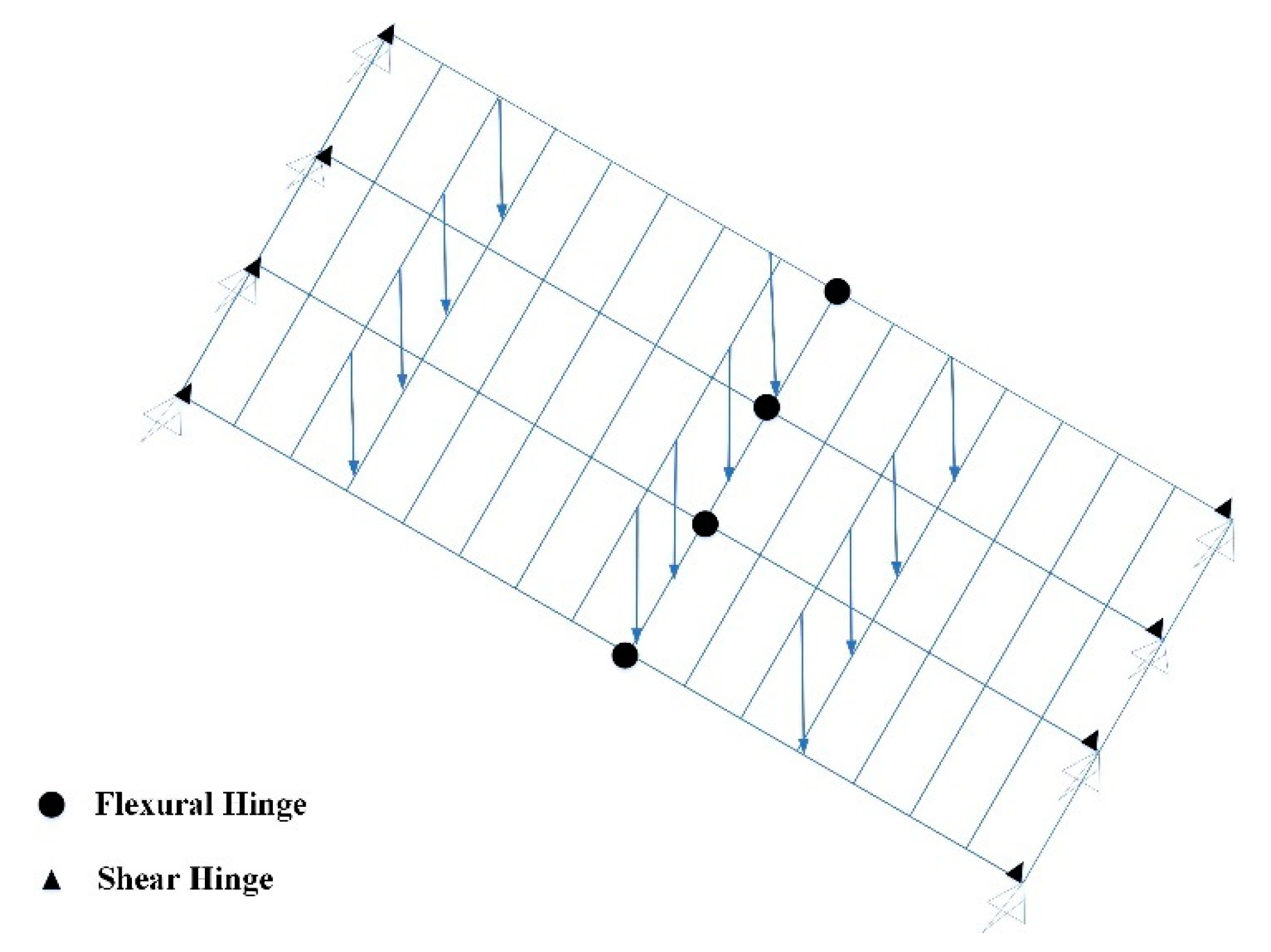
In a bridge reliability analysis, the system resistance (RSystem) is characterized as the anticipated capacity value derived from the GVW (Gross Vehicle Weight) of two entirely correlated trucks that leads to deck failure. This principle is vital for comprehending the efficacy of steel-reinforced concrete bridge decks subjected to varying loads. To design a bridge superstructure based on CHBDC-S6, flexural failure emerges as the primary mode of failure, overshadowing shear failure or excessive deflection. This phenomenon is primarily due to the susceptibility of the concrete component to crushing in the compression area or the failure of corroded steel reinforcement.

These trucks are strategically placed at a critical point on the deck of the bridge to induce the highest bending motion, with the load being incrementally risen by the time a failure mode of the deck is triggered. The anticipated values of the GVWs of trucks regarding various transverse locations are subsequently computed to establish the system resistance. This methodology is crucial for evaluating the reliability of bridge superstructures under a range of loading conditions.

The statistical load distribution for bridges serves as a basis for simulating the bridge deck’s behavior under different loading scenarios. This distribution is represented in a normal distribution format, encompassing the highest 80-year integration of dead load, live load, and dynamic load. The simulation outcomes are corroborated through a finite-element model, with the specifics of the modeling process. Figure 1 shows the Finite Element Method (FEM) employing a grillage analogy, depicting two adjacent trucks positioned on the bridge with their loads.

The Finite Element (FE) model was developed to replicate the behavior of the simply supported reinforced concrete superstructure of the bridge under a variety of loading scenarios. This model was constructed utilizing a commercial FE software package and comprised several components, including concrete beams, reinforcement, slabs, and diaphragms. The concrete beams were represented using three-dimensional solid elements with a dimension of 0.1 m and were characterized as a linear elastic material with a Young’s modulus of 30 GPa and a Poisson ratio of 0.2. The reinforcement was depicted using one-dimensional beam elements with a dimension of 0.01 m and was also treated as a linear elastic material, possessing Young’s modulus of 200 GPa and a Poisson ratio of 0.3.

Similarly, the slabs and diaphragms were modeled with three-dimensional solid elements of 0.1 m in size and were assumed to be linear elastic materials with a Young’s modulus of 30 GPa and a Poisson ratio of 0.2.

The FE model incorporated boundary conditions to replicate the bridge’s response to a range of loading scenarios, which included supports, dead load, live load, and wind load. The material characteristics utilized in the FE model were derived from the actual materials employed in the bridge’s construction.

A damage model was implemented to represent the bridge’s behavior under different loading conditions, grounded in the principles of damage mechanics, which posits that the material properties of the bridge deteriorate over time due to factors such as corrosion, fatigue, and other damage forms. This damage model was predicated on three key assumptions, namely damage initiation, damage evolution, and damage accumulation.

Additionally, a corrosion model was employed to assess the bridge’s performance under various loading conditions, based on the principles of corrosion kinetics, which suggest that the corrosion rate is influenced by factors such as the concentration of corrosive agents, temperature, and humidity. This corrosion model was also founded on three assumptions, namely corrosion initiation, corrosion evolution, and corrosion accumulation. Furthermore, a fatigue model was utilized to evaluate the bridge’s behavior under different loading conditions, based on the principles of fatigue.

3. Methodology

The suggested approach for managing the lifecycle of bridges includes a detailed system that combines five main parts, including an intervention effect model, a deterioration model, a central database, an optimization model, and a financial model. The central database is the core of this system, acting as a storage place for bridge inventory information and factors that affect how much weight the bridge can handle. This database is important for the other models, helping to forecast how the bridge will perform and assess maintenance and repair options. The deterioration model is significant because it helps predict the bridge’s reliability and condition over time. It considers various elements that contribute to bridge wear and tear, such as weather conditions, traffic loads, and material wear. By estimating how quickly a bridge deteriorates, this model helps plan when maintenance and repairs should happen. Along with predicting deterioration, the system also features an intervention effect model, which outlines how different repair methods can affect bridge performance.

This model assesses the unit costs associated with various intervention activities, facilitating the evaluation of cost-effectiveness and the enhancement of maintenance and repair strategies. The financial model serves as a crucial element of the framework, offering a systematic approach for lifecycle cost modeling and financial assessments. It incorporates a variety of expenses related to bridge ownership, such as maintenance, repair, and replacement costs.

By analyzing the financial consequences of different maintenance and repair approaches, the model aids in optimizing the lifecycle costs of bridges. Ultimately, the optimization model identifies the most economically viable maintenance and repair strategies for the bridge. It takes into account a multitude of variables and constraints, including the condition of the bridge, traffic loads, and environmental factors. Through the optimization of the objective function, the model establishes a foundation for scheduling maintenance and repair tasks that reduce lifecycle costs while maintaining the safety and performance of the bridge.

The formulation of models for bridge deterioration is significantly dependent on the presence of precise and dependable bridge inventory data. These data generally encompass circumstance scores at the component level, which have been determined through routine visual inspections of individual components. The FHWA’s (Federal Highway Administration) “Recording and Coding Guide for the Structure Inventory and Appraisal of the Nation’s Bridges” offers a standardized methodology for executing these inspections and assigning condition ratings.

In addition to visual assessments, nondestructive evaluations can also be employed to collect information regarding the condition of bridge components. By integrating the findings from these evaluations with inventory data, it becomes possible to create bridge deterioration models that forecast the future state of bridge superstructures.

The performance of a reinforced concrete bridge superstructure is affected by various parameters, such as the elasticity modulus of the reinforcing steel, the specific weight of the concrete cast in situ, the compressive robustness of the concrete, and the producing power of the reinforcing steel. Additional critical parameters include the thickness of the deck slab, the thickness of the beam web, the overall thickness of the concrete beam, and the protection of the top and bottom reinforcements in both the beam and concrete slabs. These variables have been treated as statistical parameters, with their distributions detailed in [9]. The precision of bridge deterioration models is contingent upon the quality of the input data, which include both the bridge inventory data and the outcomes of visual and nondestructive evaluations.

By adhering to standardized guidelines and protocols for the collection and analysis of these data, bridge owners and managers can create more accurate and reliable models for forecasting the future condition of their bridges.

In the following, a biquadratic deterioration curve for concrete bridge components can be formulated based on experimental data using the following formula:

$$I_{B{C}_t}=100-b_L{t}^4$$

(2)

where $t$ defines the timeline, $b_L$ represents a constant that can be ascertained through testing, and $I_{BC}$ signifies the Bridge Condition Index at time $t$, which varies in the range [0, 100].

This research presents the development of a system-level reliability-based degradation model aimed at forecasting the condition of a bridge superstructure over time. The model employs a biquadratic pattern, as articulated in Equation (3):

$${\beta }_t={\beta }_0-b{t}^4$$

(3)

where ${\beta }_0$ describes the index of reliability for a recently built bridge superstructure.

To evaluate the condition of the bridge, a condition index is utilized, which is divided into five distinct categories, namely [0, 19], [20, 39], [40, 59], [60, 79], and [80, 100]. These categories are designated as dangerous, moderate, slightly dangerous, fairly safe, and safe, respectively.

The condition index serves as a clear metric for evaluating the bridge’s state and determining the necessary interventions. For instance, a condition index ranging from 0 to 19 signifies a dangerous condition, warranting the demolition and replacement of the bridge. Conversely, a condition index of 20–39 indicates a slightly dangerous state, necessitating urgent rehabilitation of the bridge structure. The establishment of a degradation model based on system-level reliability is essential for accurately predicting the condition of a bridge superstructure and ensuring user safety. By using a biquadratic pattern, the model effectively captures the degradation process over time and offers a dependable assessment of the bridge’s condition. The pseudocode for the reliability-based degradation model is given in Algorithm 1.

Algorithm 1: The pseudocode for the reliability-based degradation model.

// Define the initial index of reliability for a recently built bridge β0 = CalculateReliabilityIndexForNewBridge ()

// Define the time-dependent reliability index βt βt = CalculateReliabilityIndexForTime (t)

// Calculate the distribution of system resistance SystemResistanceDistribution = CalculateSystemResistanceDistribution (StructuralSpecifications, ParameterVariations)

// Calculate the index of reliability for a particular time βt βt = CalculateReliabilityIndex (SystemResistanceDistribution, LoadDistribution, t)

// Apply the biquadratic degradation curve to estimate the reliability index βt βt = β0 − bt^4

// Define the primary deterioration model PrimaryDeteriorationModel = βt = β0 − bt^4

// Function to calculate the index of reliability for a recently made bridge Function CalculateReliabilityIndexForNewBridge ()     // Implement the approach for establishing a deterioration model on the basis of system-level reliability     // Return the reliability index for a newly constructed bridge End Function

// Function to calculate the index of reliability for a particular time Function CalculateReliabilityIndexForTime (t)     // Implement the procedure to estimate the reliability index for a specific time     // Return the index of reliability for the particular time End Function

// Function to calculate the distribution of system resistance Function CalculateSystemResistanceDistribution (StructuralSpecifications, ParameterVariations)     // Implement the FEM to calculate the system resistance     // Return the distribution of system resistance End Function

// Function to calculate the reliability index Function CalculateReliabilityIndex (SystemResistanceDistribution, LoadDistribution, t)     // Implement the process to predict the index of reliability     // Return the reliability index End Function

This research uses a reliability-based deterioration model for predicting the likelihood of a bridge superstructure fulfilling or surpassing its performance criteria at various intervals throughout its lifespan. The primary deterioration curve of the model can be revised following inspection outcomes over time, thereby providing a more precise depiction of the bridge’s state.

To illustrate the practical application of this model, a case study is included, focusing on a bridge superstructure designed per the Canadian Highway Bridge Design Code (CHBDC-S6). The reliability indices for this bridge are computed at two distinct points, including immediately post-construction ($t=0$) and the spalling time ($t=22$ years). The bridge superstructure features a 17 m span and a specific cross-sectional configuration. Figure 2 presents the best-fit distributions of the system resistance.

Although the biquadratic degradation model is probably viewed as a conservative method, its application in this study is justified by its straightforwardness. Employing a reliability-based deterioration model facilitates a more precise assessment of a bridge’s condition over time, empowering bridge owners and managers to make well-informed decisions relevant to maintenance and repair. By refining the model’s primary deterioration curve based on inspection findings, the accuracy of predictions can be enhanced, ultimately optimizing the bridge’s performance.

In bridge maintenance, both significant and minor interventions are essential for prolonging the lifespan of the structure. Minor interventions, such as the patching and sealing of surfaces of the concrete deck, can be executed during partial traffic closures and have demonstrated an enhancement in the reliability index by as much as 0.2. Conversely, major interventions, which include increasing the thickness of concrete cover and the application of laminates of Fiber-Reinforced Polymer (FRP), necessitate comprehensive traffic closure because of the specialized methods required.

While certain studies declared that major interventions could restore a bridge’s reliability index to its original state, others indicated that the deterioration model could experience a step function growth within the major intervention time, leading to the index of a condition (and index of reliability) reaching up to 0.95 of a defect-free state.

To ascertain the necessity of a major intervention, a threshold value of ${\beta }_t\in [0.2{\beta }_0,0.4]$ is employed, signifying that the bridge structure is in a slightly hazardous condition and requires a major intervention. In contrast, if the reliability index drops below $0.2{\beta }_0$, the bridge is deemed to be in a perilous state and necessitates complete replacement, which is not included in the simulations of this study.

The influence of both major and minor interventions on a bridge’s reliability index is a vital aspect of maintenance planning. By comprehending the ramifications of these interventions, bridge owners and managers can make well-informed decisions regarding the timing and methods of maintenance activities to enhance the bridge’s longevity.

To guarantee the safety and effective lifecycle management of a bridge, it is crucial to establish a deterioration model based on system reliability that aligns with the costs associated with lifecycle maintenance and rehabilitation. This model must consider the effects of both major and minor intervention activities on the bridge’s lifespan, as various combinations of these interventions can lead to different structural lifetimes.

To measure the feasibility of various intervention scenarios, logical criteria should be employed to evaluate their lifecycle costs. This evaluation is particularly significant when analyzing multiple intervention options, as a lifecycle cost optimization approach can help identify the most advantageous alternative. One effective method for this purpose is the Equivalent Uniform Annual Worth (EUAW) approach, which aggregates all future costs into uniform annual payments throughout the analysis period. The EUAW method serves as a valuable tool for decision-makers, enabling them to compare alternatives with differing anticipated lifecycles. Here, it is assumed that the starting capital expenditures for each alternative are identical, and the EUAW is computed using the specified formula.

$$EUAW={\displaystyle \frac{\sum \left(\frac{C_t}{{\left(1+i\right)}^t}\right)}{n}}$$

(4)

where $C_t$ represents the cost within t^th time, $n$ denotes the interval of the network’s lifecycle, and $i$ refers to the rate of interest, which is supposed to be 0.06 for this study.

Using the EUAW method allows decision-makers to assess the lifecycle costs associated with various intervention scenarios, thereby facilitating the identification of the most economically viable option. This methodology promotes the optimization of lifecycle costs, ensuring that the bridge is maintained and rehabilitated in a manner that is both safe and financially prudent.

The bridge superstructure examined in this case study is a simply supported reinforced concrete structure featuring a span of 18 m. It is engineered to support a load of 300 kN/m² and has an overall width of 10 m. The superstructure is composed of four reinforced concrete beams, each measuring 0.5 m in width and 1.5 m in height, arranged with a spacing of 2.5 m and resting on two piers at either end. These beams are reinforced with steel bars of 16 mm diameter, possessing a yield strength of 500 MPa, arranged in a rectangular configuration with a spacing of 200 mm.

The concrete used has a compressive strength of 30 MPa and an elasticity modulus of 30,000 MPa. The bridge deck consists of a 200 mm thick reinforced concrete slab, supported by the four beams, and is designed to accommodate the same load as the superstructure. The piers have a diameter of 1.5 m and a height of 10 m, are established on a pile foundation, and are intended to transfer the loads from the superstructure to the foundation. The foundation comprises piles that are 1.5 m in diameter, 20 m in length, and spaced 2.5 m apart. They effectively transfer loads to the underlying clay soil, which has a modulus of elasticity of 5000 MPa and a Poisson ratio of 0.3.

The deterioration model based on reliability used in this research is a probabilistic framework that forecasts the degradation of the bridge superstructure over time, relying on several essential parameters. The deterioration rate, which is a pivotal factor influencing the degradation speed, is presumed to adhere to a normal distribution characterized by a mean of 0.05 and a standard deviation of 0.01. It is assumed that the initial state of the bridge superstructure is satisfactory, with a failure probability of 0.01. The model projects the deterioration over one year, employing a time step of one year and conducting 1000 simulations.

This framework operates as a Markov chain model, which represents the deterioration of the bridge superstructure through transition probabilities derived from the deterioration rate and initial condition, along with a state space comprising discrete states that depict the condition of the bridge superstructure. The model presumes a constant deterioration rate throughout the timeframe, a normal distribution of these rates, and the independence and identical distribution of deterioration rates. Furthermore, it is assumed that no maintenance activities are undertaken on the bridge superstructure and that external influences, such as weather, traffic, or other environmental factors, do not impact the deterioration rate.

4. Improved Electric Fish Optimization

4.1. Background

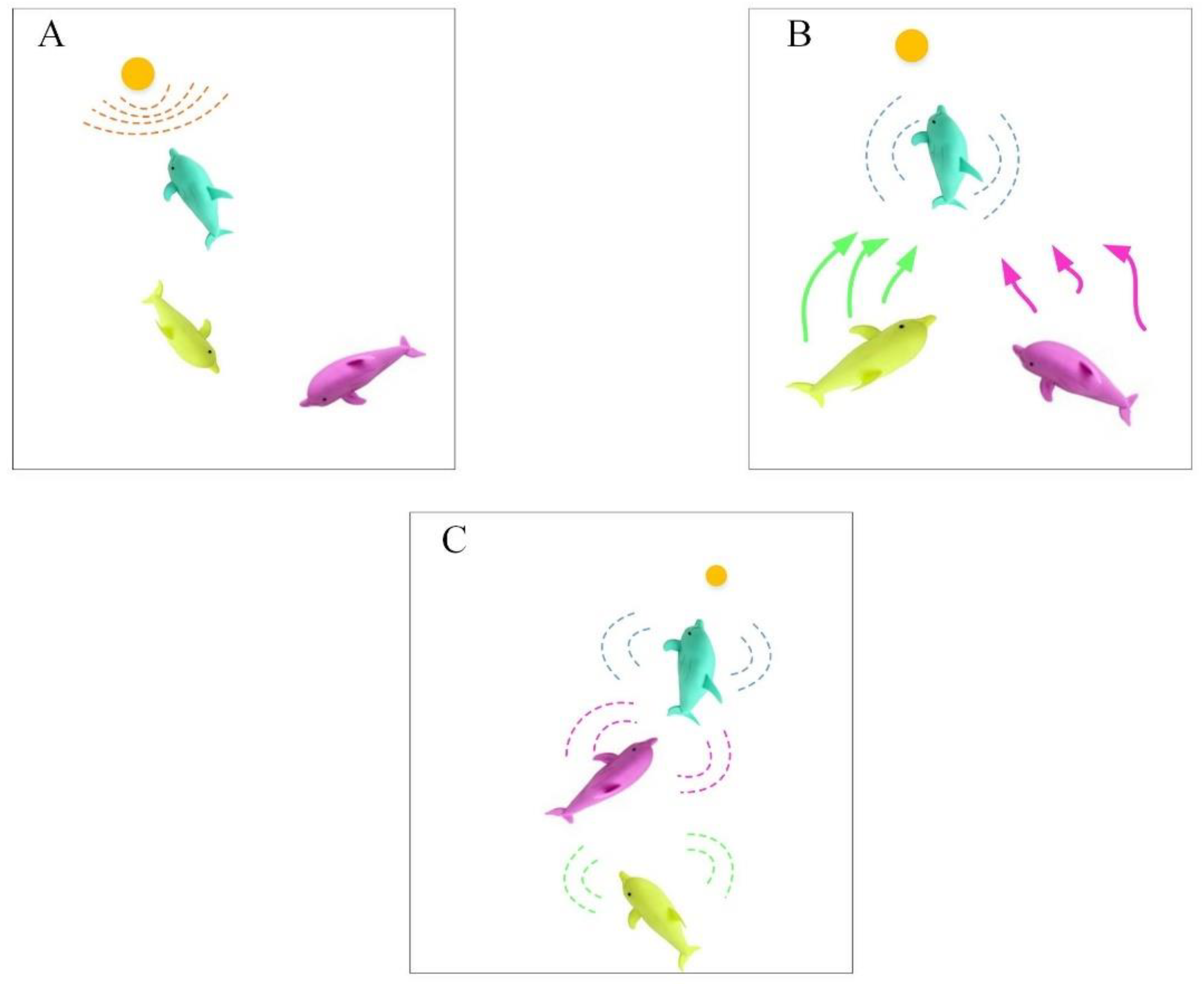
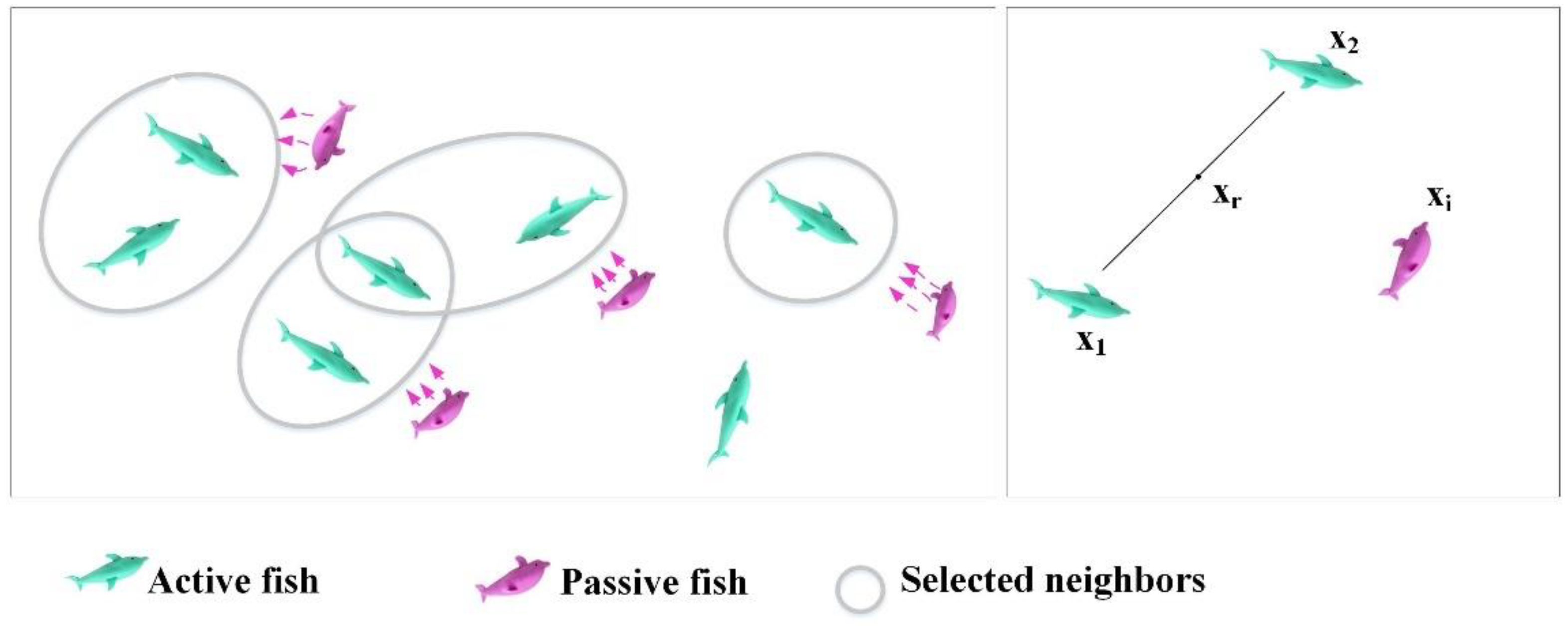
Electric fish make up only a small portion of fish kinds. They inhabit muddy water, where their vision is limited, and most of them are active at night. But they have a species-specific ability, electrolocation, which is the unique sense they rely on to situate objects, such obstacles and prey. Electric fish are divided into weakly and strongly electric fish, based on the power of the electric field they produce. Strongly candidates mainly employ electrolocation for attacking aims, and their ground intensity is between 10 and 600 V, enough to stun the target. Conversely, weak candidates produce electric grounds of intensity between a few volts and a few hundred millivolts, employed for object detection, communication, navigation, and more.

The heuristics share the same framework. However, the utility of search procedures is based on the specific model, which distinguishes heuristics. Electric Fish Optimization (EFO) follows this pattern and employs straightforward search processes. The algorithm’s specifics have been outlined in the following. Initially, the assumptions that adapt the manner of these animals into the heuristic optimizer, reflecting their innate characteristics, are presented. The initial premise is that there exists an unlimited nutrition supply within the solution space, with one nutrition source standing out as the superior option. Figure 3 illustrates the processes of communication and target identification within a fish swarm.

These animals, representing the candidates, have been positioned in the area and retain information about their locations. Each individual’s quality has been ascertained by its proximity to the best nutrition source, then the most important issue is to find the highest quality nutrition source. Additionally, drawing inspiration from natural evolution, another assumption is that individuals with access to high-quality resources for an extended period of time experience accelerated growth and generate signals of electricity with greater amplitudes compared with their counterparts.

The smart manners of these animals have been explained in the following:

-

Active electrolocation. These animals are capable of producing regular signals of electricity by employing their organs. Active electrolocation is in a constrained range; as a result, it is utilized to ensure exploitation by employing candidates that have better cost values in a way that they are more skilled to explore their immediate surroundings.

-

Passive electrolocation. Initially, it should be mentioned that other animals do not have such an ability to produce electricity; however, they depend on the electric signal that stems from animate organisms of conspecific electric organ. Since the passive electrolocation owns a more extended range in comparison with the active one, it is utilized in the present optimizer to balance active electrolocation and ensure exploration skills by empowering all candidates to have wide exploration; moreover, candidates with low fitness value have priority.

-

OD frequency. In the natural environment, the rate at which electric fields are produced is influenced by proximity to the source. Fish in the closest proximity to the most favorable source have been assumed to generate electric fields more regularly compared with others. The frequency EOD is utilized in EFO to assess the function of all individuals at a specific time $t$, since it serves as an indicator for these animals to identify which candidates are near a superior nutrition source. Just like natural life, the candidates that have more frequency utilize active electrolocation and the other individuals utilize a passive one.

-

EOD amplitude. The size of these animals affects the amplitude of the electric ground, which in turn influences the efficient variety of the electrical stimuli. The EOD’s amplitude is utilized in the EFO algorithm to establish the dominance of electric ground, determining the effective range for exploitation and the likelihood of candidates being detected in exploration.

At first, the population of these animals $\left(N\right)$ was stochastically distributed within the solution space by considering the limitations of the area.

$$x_{ij}=x_{minj}+\varphi (x_{maxj}-x_{minj})$$

(5)

where the situation of the i^th candidate within the population has been indicated via $x_{ij}$ that has the size of $\left|N\right|(i=1, 2, . . ., |N|$ within a solution space with $d$ dimensions. $x_{maxj}$ and $x_{minj}$ have been found to be upper and lower limitations within dimension $j| j\in 1, 2,\dots ,d$. Moreover, $\varphi$ is between zero and one; it is a stochastic value and is taken when there is a uniform distribution.

Once the initialization stage has been accomplished, members of the population navigate the solution space using their passive or active electrolocation ability. The EFO uses frequency to strike a balance between exploitation and exploration, determining whether a candidate will engage in passive or active electrolocation. This prioritizes more capable candidates (active candidates) to exploit their surroundings and potentially promising areas, while encouraging other candidates (passive candidates) to explore the search space and uncover novel areas, which is crucial for multimodal functions.

In the present optimizer, the candidates that have higher frequency skills utilize active electrolocation, while other candidates employ passive electrolocation. A candidate’s value of frequency is between a maximum value $f_{max}$ and a minimum value $f_{min}$. Since a candidate’s value of frequency within time $t$ is highly relevant to its nearness to the nutrition source, a candidate’s value of frequency $\left(f_i^t\right)$ results from its fitness value of it in the following manner:

$$f_i^t=f_{min}+\left({\displaystyle \frac{fi{t}_{worst}^t-fi{t}_i^t}{fi{t}_{worst}^t-fi{t}_{best}^t}}\right)\left(f_{max}-f_{\mathrm{m}\mathrm{i}\mathrm{n}}\right)$$

(6)

where the best and worst fitness values have been, in turn, $fi{t}_{best}^t$ and $fi{t}_{worst}^t$ gained from candidates within the present population within $t^{th}$ iteration, while $i^{th}$ candidate’s fitness value within $t^{th}$ iteration has been displayed via $fi{t}_i^t$. In the present investigation, the value of frequency was employed for a possible computation; $f_{max}$ and $f_{min}$ are, in turn, 1 and 2.

In addition to the frequency, these animals have some information relevant to amplitude, as well. This can determine the active variety of a fish while they are electrolocating in an active manner, and the possibility of being understood by several passively electrolocating animals when the power of electric context declines with the distance’s opposite cube.

The weight of the candidate’s prior amplitude determines a candidate’s amplitude. Consequently, it might not get altered that much. Candidate $i$’s amplitude value is computed in the following manner:

$$A_i^t=\alpha A_i^{t-1}+\left(1-\alpha \right)f_i^t$$

(7)

where the constant value is illustrated by $\alpha | \alpha \in [0, 1]$, which can determine the scope of the prior amplitude value. In the present algorithm, candidate $i$’s initial amplitude value is initiated with the initial value of frequency $f_i$.

The amplitude and frequency variable values of a candidate are upgraded based on the immediacy of the candidates to the finest target source. In each iteration of the optimizer, the population is separated into two groups based on each candidate’s value of frequency, including the candidates implementing passive (NP) and active electrolocation (NA), which means $N_A\cup N_P=N$. Since the candidate’s frequency is contrasted with a stochastic value that has been distributed uniformly, it is more possible to implement active electrolocation if a candidate’s frequency value is higher. The exploration is implemented by candidates within $NP$ and $NA$ in a parallel mode.

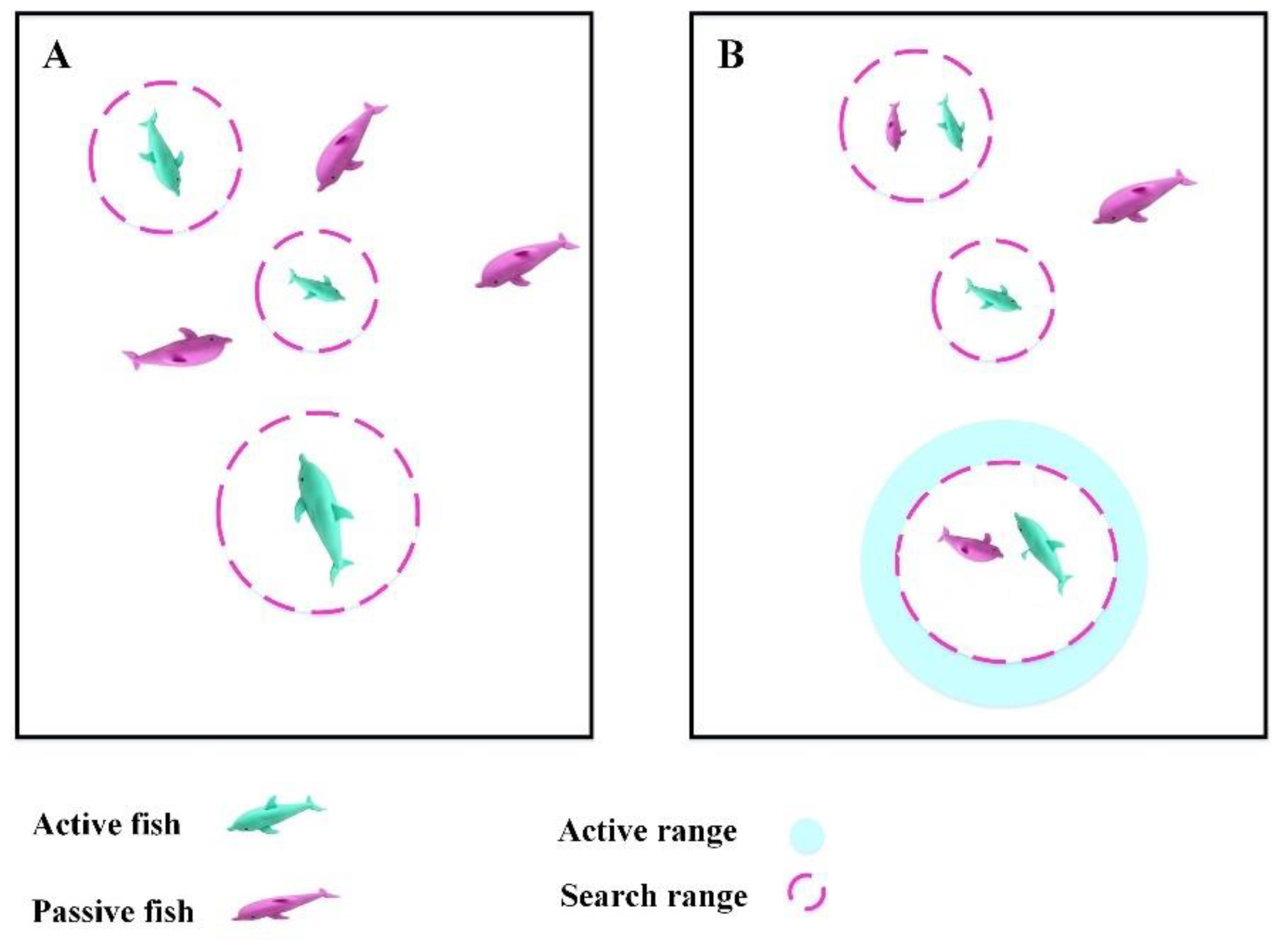
4.2. Active Electrolocation

The efficient variety of $PA$ is constrained to nearly half of the animal, and the candidate cannot find the target exterior of the previously determined boundary. In other words, this skill enables the candidates to situate all nutrition sources in their neighborhood. The exploitation skill of the present algorithm is based on the features of the $PA$.

In the present algorithm, each individual acting as $PA$ changes its position in the solution space by enhancing its manner. However, merely one variable randomly selected can be enhanced when the candidates go to distant areas.

The motion of candidate $i$ might be different based on the presence of the neighbors in its active boundary. If there is no neighbor, it implements a stochastic walk inside its boundary. Otherwise, it selects one neighbor in a random manner and alters its situation on the basis of that neighbor. The optional exploration is the “explore first, exploit later” method in the present algorithm. Figure 4 illustrates the local search process of the EFO.

Since there is a large distance between the candidates in the beginning, they are not in active boundaries with each other in most cases. Consequently, it is probable that active candidates initially search their vicinity stochastically, then they commence exploiting the nearest area while the number of iterations increases.

The active boundary of the $i^{th}$ candidate $\left(r_i\right)$ is ascertained via its amplitude value $\left(A_i\right)$. The active boundary can be calculated subsequently:

$$r_i=\left(x_{maxj-x_{minj}}\right)A_i$$

(8)

To discover candidates in the same vicinity $\left(S\right| S\subset N)$ in an active boundary, the distance between the rest of the population and candidate $i$ must be measured, which means $N/\left[i\right]$. The distance between the candidates $k$ and $i$ is ascertained by subsequently employing Cartesian distance computation:

$$d_{ik}=||x_i-x_k=\sqrt{{\sum }_{j=1}^d{\left(x_{ij}-x_{kj}\right)}^2}$$

(9)

Here, when there is only one area in the active boundary at minimum, Equation (10) is employed. Else, $S=\varnothing$.

$$x_{ij}^{cand}-x_{ij}+\phi (x_{kj}-x_{ij})$$

(10)

where $\phi$ is found to be a stochastic number produced from a uniform distribution, which is between −1 and 1. Moreover, the individual situation of candidate $i$ is indicated via $x_{ij}^{cand}$.

4.3. Passive Electrolocation

In contrast to active electrolocation, the sensing remoteness is not influenced by candidate $i$ and extends above the boundary of active electrolocation. For this reason, the passive electrolocation skill meets the needs of the exploration approach of the suggested algorithm. Figure 5 shows the global search demonstration of the EFO.

It has been previously stated that the likelihood of a signal being detected is linked to both its distance and its amplitude from the intended candidate. Passive individuals select active individuals who transmit electrical signals based on a specific possibility and then proceed to alter their positions.

The possibility that $k^{th}$ active candidate $(k\in NA)$ has been perceived via $i^{th}$ passive candidate $(i\in NP)$ can be computed subsequently:

$$p_k={\displaystyle \frac{\frac{A_k}{d_{ik}}}{\sum _{j\in N_A}\frac{A_j}{d_{ij}}}}$$

(11)

It can be seen that passive electrolocation utilizes a distance-based choosing approach and an amplitude-based choosing like the gravitational search algorithm and firefly algorithm. It should be noted that probabilistic neighbor choosing urges passive candidates to implement global search before local search. As a result, passive candidates select near candidates within the starting iterations, since remoteness is the key element that causes the choice of worse candidates, contributing to the discovery of novel areas within the solution space. Amplitude becomes the key element while the number of iterations increases, causing the choice and best candidates’ exploitation.

Employing diverse techniques, like roulette wheel selection, $K$ candidates have been selected from $NA$ based on Equation (11). After that, a reference situation $x_{rj}$ is ascertained based on Equation (12). Consequently, the new situation is produced by employing Equation (13).

$$x_{rj}={\displaystyle \frac{{\sum }_{k=1}^K{A}_k{x}_{kj}}{{\sum }_{k=1}^K{A}_k}}$$

(12)

$$x_{ij}^{new}=x_{ij}+\phi \left(x_{rj}-x_{ij}\right)$$

(13)

In contrast to the search involved in active electrolocation, individuals can modify more than one variable to explore the solution space quickly. On the other hand, in rare cases, a scenario may occur where a candidate with more frequency engages in passive electrolocation. This situation could lead to the loss of situation data for the individual, which is unexpected given the promising location. In order to prevent this from happening, EFO uses Equation (14) to ascertain the variables that are going to be enhanced. As part of the acceptance status, the probability of the individual modifying its entire characteristic is considerably reduced.

$$x_{ij}^{cand}=\left\{\begin{array}{c}{x}_{ij}^{new} ran{d}_j(0, 1)>f_i\\ x_{ij} else \end{array}\right.$$

(14)

Here, a uniform stochastic quantity is demonstrated by $ran{d}_j(0, 1)$, produced for the variable $j$.

The ultimate stage of passive electrolocation is modifying one variable of the individual $i$ by employing Equation (15) with the purpose of increasing the possibility of a trait that is altered.

$$x_{ij}^{cand}-x_{minj}+\phi \left(x_{maxj}-x_{minj}\right), rand\left(0, 1\right)\le rand(0, 1)$$

(15)

where $rand(0, 1)$ is found to be a stochastically produced quantity which is achieved by the uniform distribution.

Once the variable $j$ value of candidate $i$ surpasses the limitation of the solution space, it is relocated at the limitation of the area, which it surpasses in the following way:

$$x_{ij}^{cand}=\left\{\begin{array}{c}{x}_{minj} x_{ij}^{cand}<x_{minj} \\ x_{ij}^{cand} x_{maxj}>x_{ij}^{cand}>x_{minj}\hfill \\ x_{maxj} x_{ij}^{cand}>x_{maxj} \hfill \end{array}\right.$$

(16)

The current stages, active and passive, ascertain the complexity of the suggested optimizer. The stages’ complexities are largely manipulated via the distance computation of the candidates. Thus, the passive and active stages’ complexities of time are, in turn, illustrated by $O(\left|N_P\right|\times \left|N_A\right|)$ and $O\left(\left|N_A\right|\times \left|N\right|\right)$. Additionally, the optimizer owns a complexity that has been found to be proportional to the variable $O\left(\right|N\left|\right)$ for the evaluation of the fitness of the population. In brief, the suggested algorithm’s complexity of time has been found to be $O\left({\left|N\right|}^2\right)$ and $O\left(\left|N\right|\right)$ for worst and best cases when the $\left|N_A\right|$ equals $\left(\left|N\right|-1\right)$ and 1, respectively.

4.4. Improved Electric Fish Optimization (IEFO)

The original Electric Fish Optimization algorithm may face some limitations, such as balance issues and untimely isotropy, that affect how the Electric Fish Optimization algorithm works. These problems led us to develop an enhanced version of the algorithm aimed at overcoming these challenges as much as possible [15]. In this study, we utilized the Lévy Flight (LF) function as a chaotic mechanism to boost the algorithm’s efficiency [16]. The Lévy Flight creates a random walk process that helps fine-tune local exploration, as shown in the following equations [17].

$$\mathrm{L}\mathrm{e}\left(w\right)\approx {\displaystyle \frac{1}{{\mathrm{w}}^{1+\mathsf{\xi }}}}$$

(17)

$$\mathrm{w}={\displaystyle \frac{\mathrm{A}}{{\left|\mathrm{B}\right|}^{1/\mathsf{\xi }}}}$$

(18)

$${\mathsf{\sigma }}^2={\left\{{\displaystyle \frac{\mathsf{\Gamma }(1+\mathsf{\xi })}{\mathsf{\xi }\mathsf{\Gamma }\left(\right(1+\mathsf{\xi })/2)}}{\displaystyle \frac{\mathrm{s}\mathrm{i}\mathrm{n}(\mathsf{\pi }\mathsf{\xi }/2)}{2^{(1+\mathsf{\xi })/2}}}\right\}}^{{\displaystyle \frac{2}{\mathsf{\xi }}}}$$

(19)

where $\xi$ is a value that falls between 0 and 2, $A$ and $B$ are normally distributed with a mean of 0 and a variance of ${\sigma }^2$, $\mathsf{\Gamma }\left(\right(1+\mathsf{\xi })/2)$ represents the Gamma function, the variable $w$ stands for the step size, and $\xi$ indicates the Lévy index. As stated in [18], the value of ξ is quantified as 3/2.

$$x_{ij}^{can{d}_{New}}=x_{ij}^{cand}+(x_{ij}^{cand}-AD)\times \mathrm{L}\mathrm{e}(\mathsf{\delta })$$

(20)

where $x_{ij}^{can{d}_{New}}$ describes the new position for the new selected member,

$$A=a\times (2\times r-1)$$

(21)

$$D=C\times \widehat{\mathrm{x}}-x_{ij}^{cand}$$

(22)

where $r$ specifies the random rate ranging between 0 and 1, $\widehat{\mathrm{x}}$ represents a vector for random position from the existing single, and $\gamma$ is considered 1 (which is between 0 and 2).

To ensure the best results have been achieved, progress has been made, shown as follows:

$$x_{ij}^{cand}=\left\{\begin{array}{c}{x}_{ij}^{cand} F\left(x_{ij}^{New}\right)>F\left(x_{ij}\right)\\ x_{ij}^{can{d}_{New}} otherwise\end{array}\right.$$

(23)

The IEFO algorithm employs the Lévy Flight (LF) function as a chaotic mechanism to enhance its efficiency, facilitating a random walk process that refines local exploration. The Lévy Flight is characterized by Equations (20)–(22). The IEFO algorithm offers a more efficient and effective optimization approach compared with the original EFO algorithm, enabling enhanced local exploration and improved results.

4.5. Maintenance Planning Based on IEFO

In this study, due to the problem’s complexity, the IEFO algorithm was employed. The characteristics of the optimization model must meet these seven criteria. The optimization model for bridge superstructure maintenance and rehabilitation must satisfy some important criteria to ensure the longevity and safety of the structure. These criteria are on the basis of the CHBDC-S6 and are designed to optimize the rehabilitation and maintenance strategy for the bridge.

To start, the bridge superstructure needs to last at least 80 years, in accordance with CHBDC-S6. This requirement ensures that the bridge was built to endure over time and keep users safe. Next, the reliability index (${\beta }_t$) should be between $[$0.2${\beta }_0$, 0.4${\beta }_0]$, which signals a slightly risky situation that calls for major repairs. This range is essential for spotting when significant maintenance is needed to avoid serious failures. Also, if the reliability index (${\beta }_t$) is between 0.8${\beta }_0$ and ${\beta }_0$, it shows that the bridge is in a safe state, meaning that no repairs are necessary.

This range serves as a standard for assessing the bridge’s safety and reliability. Furthermore, a reliability index (β_t) of $0.2\beta 0$ or lower points to a dangerous situation that is not acceptable and needs urgent action. Also, the range from $0.79\beta 0$ to $0.2\beta 0$ reflects fairly safe conditions, moderate, and slightly dangerous, where minor maintenance tasks can be performed to keep the structure in good shape. Any solutions that require small intervention activities over several years are considered unsuitable and will not be taken into account.

This helps to make sure that the maintenance and repair plan is as efficient as possible, avoiding unnecessary and expensive actions. After 80 years, no more intervention actions are carried out since it is believed that the bridge superstructure has reached the end of its useful life. By meeting these standards, the optimization model can create a thorough and effective maintenance and repair strategy for the bridge superstructure, ensuring that the structure remains safe and lasts a long time.

In this study, the proposed IEFO algorithm was suggested to minimize the Equivalent Uniform Annual Worth ($W_{EUA}$) of costs associated with bridge maintenance:

$$W_{EUA}=\sum _{t=1}^n{\displaystyle \frac{C_t}{{\left(1+i\right)}^t}}\times {\displaystyle \frac{i{\left(1+i\right)}^t}{{\left(1+i\right)}^t-1}}$$

(24)

The objective was to strategically select intervention alternatives at different time points to balance structural integrity and economic feasibility. The chosen interventions, indicated by a carefully designed IEFO algorithm fitness function, include major and minor repairs.

Major interventions are reserved for more severe structural conditions, while minor interventions address cracks and other signs of deterioration. The bridge superstructure’s design life span of 80 years is carefully considered, with no interventions implemented beyond this timeframe.

4.6. Algorithm Validation

This section aims to demonstrate the superiority of the proposed IEFO algorithm for feature selection in comparison with other algorithms. To ensure a comprehensive analysis, six distinct standard benchmark functions were used, comprising two Unimodal functions in 30 dimensions, two Multimodal functions in 30 dimensions, and two Multimodal functions in lower dimensions. The results obtained from these functions were then compared with several advanced methodologies, including the Reptile Search Algorithm (RSA) [19], $\beta$-hill climbing ($\beta$-HC) [20], Lévy Flight Distribution (LFD) [21], and Golden Sine Algorithm (GSA) [22].

The parameter settings of the studied algorithms are expressed in the following. The Reptile Search Algorithm (RSA) uses an alpha value of 0.1 and a $\beta$ value of 0.01, while the $\beta$-hill climbing ($\beta$ HC) algorithm uses a $\beta$ value of 0.05 and a bandwidth ($bw$) of 0.5. The Lévy Flight Distribution (LFD) algorithm has a threshold value of 2, a Coefficient of Variation (CSV) of 0.5, a $\beta$ value of 1.5, and alpha values of 10, 0.00005 and 0.005, respectively. Additionally, the LFD algorithm uses delta values of 0.9 and 0.1. The Golden Sine Algorithm (GSA) uses a gravitational constant of 100 and a decreasing coefficient of 20. These parameter settings are used to optimize the performance of the respective algorithms in this study.

The simulation was conducted independently 20 times for each algorithm and function to ensure dependable results for comparison purposes.

Table 1. The benchmark functions employed along with their target values ($f_{min}$) and associated constraints for evaluation.

Function	Range	$${\mathit{f}}_{\mathit{m}\mathit{i}\mathit{n}}$$
$F_1(X)={\displaystyle \sum _{i=1}^{n-1}}\left[100{\left(x_{i+1}-x_i^2\right)}^2+{\left(x_i-1\right)}^2\right]$	$${\left[-\mathrm{30,30}\right]}^n$$	0
$F_2(X)={\displaystyle \sum _{i=1}^{n-1}}\left[{\left(x_i+0.5\right)}^2\right]$	$${\left[-\mathrm{100,100}\right]}^n$$	0
$F_3(X)={\displaystyle \sum _{i=1}^{n-1}}\left(x_i^2-10\cos 2\pi x_i+10\right)$	$${\left[-\mathrm{5.12,5.12}\right]}^n$$	0
$$\begin{gathered} F_4\left(X\right)=0.1\left[{\sin }^{2}3\pi x_1+{\displaystyle \sum _{i=1}^n}{\left(x_i-1\right)}^2\left(1+{\sin }^2\left(3\pi x_1+1\right)\right)+{\left(x_n-1\right)}^2\left(1+{\sin }^2\left(2\pi x_n\right)\right)\right] \\ +{\displaystyle \sum _{i=1}^n}u\left(x_i,\mathrm{5,100,4}\right) \end{gathered}$$	$${\left[-\mathrm{50,50}\right]}^n$$	0
$F_5(X)={\left(x_2-{\displaystyle \frac{5.1}{4{\pi }^2}}{x}_1^2+{\displaystyle \frac{5}{n}}{x}_1-6\right)}^2+10\left(1-{\displaystyle \frac{1}{8\pi }}\right)\cos x_1+10$	$${\left[-5,15\right]}^2$$	3979
$\begin{array}{l}{F}_6\left(X\right)=-{\displaystyle \sum _{i=1}^4}{c}_i\exp \left(-{\displaystyle \sum _{j=1}^6}{a}_{ij}{\left(x_j-p_{ij}\right)}^2\right)\\ \hspace{1em}\hspace{1em}\hspace{1em}\hspace{1em}\hspace{1em}\hspace{1em}\hspace{1em}\hspace{1em}\hspace{1em}{a}_{ij}=\left(\begin{array}{c}10,3,17,3.5,1.7,8\\ 0.05,10,17,0.1,8,14\\ \begin{array}{c}3,3.5,1.7,10,17,8\\ 17,8,0.05,10,0.1,14\end{array}\end{array}\right), c_i=\left[1,1.2,3,3.2\right]\\ p_{ij}=\left(\begin{array}{c}0.1312,0.1696,0.5569,0.0124,0.8283,0.5886\\ 0.2329,0.4135,0.8307,0.3736,0.1004,0.9991\\ \begin{array}{c}\mathrm{0.2348,0.1415},0.3522,0.2883,0.3047,0.6650\\ 0.4047,0.8828,0.8732,0.5743,0.1091,0.0381\end{array}\end{array}\right)\end{array}$	$${\left[\mathrm{0,1}\right]}^6$$	−3.32

presents the benchmark functions employed along with their target values ($f_{min}$) and the associated constraints for evaluation [23].

To ensure a fair comparison, the population size of all algorithms was established at 50, with each algorithm undergoing 200 iterations. The results of the simulation analysis are presented in

Table 2. Results of the comparative analysis conducted on the examined benchmark functions.

Function	Metric	RSA	β-HC	LFD	GSA	IEFO
$F_1$	Mean	9.73 × 102	3.37 × 104	5.37 × 101	4.25 × 101	3.02 × 101
	Min	2.14 × 102	1.24 × 102	4.50 × 101	2.31 × 101	1.62 × 101
	Var	4.06 × 105	3.03 × 105	2.01 × 105	6.19 × 10−1	5.03 × 10−1
$F_2$	Mean	2.37 × 101	1.84 × 10−3	2.75 × 100	1.83 × 100	0.00 × 100
	Min	1.51 × 101	1.55 × 10−4	6.64 × 10−1	4.59 × 10−1	0.00 × 100
	Var	2.69 × 101	1.73 × 10−4	8.71 × 100	8.19 × 100	0.00 × 100
$F_3$	Mean	4.47 × 10−1	7.69 × 10−1	4.67 × 10−1	2.52 × 10−3	4.05 × 10−4
	Min	4.04 × 10−1	5.93 × 10−1	3.23 × 10−1	2.79 × 10−4	3.85 × 10−5
	Var	1.71 × 10−3	2.50 × 10−3	6.01 × 10−3	3.97 × 10−7	4.46 × 10−8
$F_4$	Mean	1.11 × 10−1	7.24 × 10−2	2.51 × 10−3	4.52 × 10−6	3.06 × 10−18
	Min	6.67 × 10−2	4.49 × 10−2	3.68 × 10−5	3.80 × 10−7	2.43 × 10−18
	Var	6.99 × 10−4	6.39 × 10−4	6.05 × 10−6	8.49 × 10−8	2.71 × 10−20
$F_5$	Mean	6.18 × 10−1	5.41 × 10−1	5.39 × 10−1	5.68 × 10−1	5.22 × 10−1
	Min	6.38 × 10−1	6.03 × 10−1	5.85 × 10−1	5.67 × 10−1	5.26 × 10−1
	Var	1.31 × 10−8	5.94 × 10−10	4.88 × 10−11	3.77 × 10−12	5.13 × 10−14
$F_6$	Mean	−5.23 × 100	−4.39 × 100	−4.54 × 100	−4.11 × 100	−3.40 × 100
	Min	−4.01 × 100	−3.71 × 100	−3.76 × 100	−3.80 × 100	−3.67 × 100
	Var	2.37 × 10−3	2.10 × 10−3	1.69 × 10−3	1.24 × 10−3	1.20 × 10−3

. This analysis takes into account the mean value, the minimum value, and the variance.

The results presented in Table 2 illustrate the dominance of the IEFO algorithm compared with other algorithms regarding mean, minimum, and variance values across all functions. The IEFO algorithm consistently exhibits the lowest mean and minimum values, signifying its effectiveness and efficiency. Furthermore, it also records the lowest variance values, highlighting its consistency and reliability. In contrast, the RSA displays the highest mean and variance values for the majority of functions, suggesting that it is the least consistent and reliable option.

While the $\beta$-HC, LFD, and GSA show lower mean and variance values than the RSA, they still fall short of the performance demonstrated by the IEFO algorithm. The data indicate that the IEFO algorithm surpasses its counterparts in most instances, maintaining the lowest mean and variance values across all functions. For instance, in function F1, the IEFO algorithm achieved a mean value of 3.02 × 10¹, which was markedly lower than the mean values of the other algorithms, such as the RSA (9.73 × 10²), $\beta$-HC (3.37 × 10⁴), LFD (5.37 × 10¹), and GSA (4.25 × 10¹).

Likewise, in function F2, the IEFO algorithm recorded a mean value of 0.00 × 10⁰, the lowest among all algorithms. The results further confirm that the IEFO algorithm possesses the lowest minimum values for all functions, reinforcing its status as the most effective algorithm for identifying optimal solutions. In summary, the results in Table 2 affirm the superiority of the IEFO algorithm over its competitors, positioning it as a promising approach for addressing optimization challenges.

The proposed IEFO algorithm has also been compared with other optimization techniques in terms of convergence speed and solution quality.

Table 3. Average comparison of IEFO with other optimization techniques for the functions.

Algorithm	Convergence Speed	Solution Quality
IEFO	0.05	0.0001
GSA	0.12	0.0012
LFD	0.20	0.0025
$\beta$-HC	0.15	0.0018
RSA	0.10	0.0015

indicates the average comparison of IEFO with other optimization techniques regarding the functions.

The IEFO algorithm demonstrated superior performance compared with the GSA in terms of both convergence speed and solution quality, achieving a convergence speed that was 2.4 times quicker and a solution quality that was 12 times more effective. Furthermore, the IEFO algorithm surpassed the LFD algorithm in these metrics, exhibiting a convergence speed that was 4 times faster and a solution quality that was 25 times better.

In addition, the IEFO algorithm outperformed the $\beta$-HC algorithm, with a convergence speed that was 3 times faster and a solution quality that was 18 times superior. Lastly, when compared with the RSA, the IEFO algorithm showed a convergence speed that was 2 times faster and a solution quality that was 15 times better. The findings presented in Table 3 highlight the IEFO algorithm’s dominance over other optimization methods regarding both convergence speed and solution quality, establishing it as a highly effective and dependable optimization approach.

5. Simulation Results

This study used the established deterioration and optimization models in a case study directed at a fundamentally supported reinforced concrete superstructure of a bridge, which was constructed according to the simple guidelines of the CHBDC-S6. The selected structural configuration is indicative of a substantial quantity of existing bridges across the United States and Canada, characterized by a simply supported concrete beam arrangement.

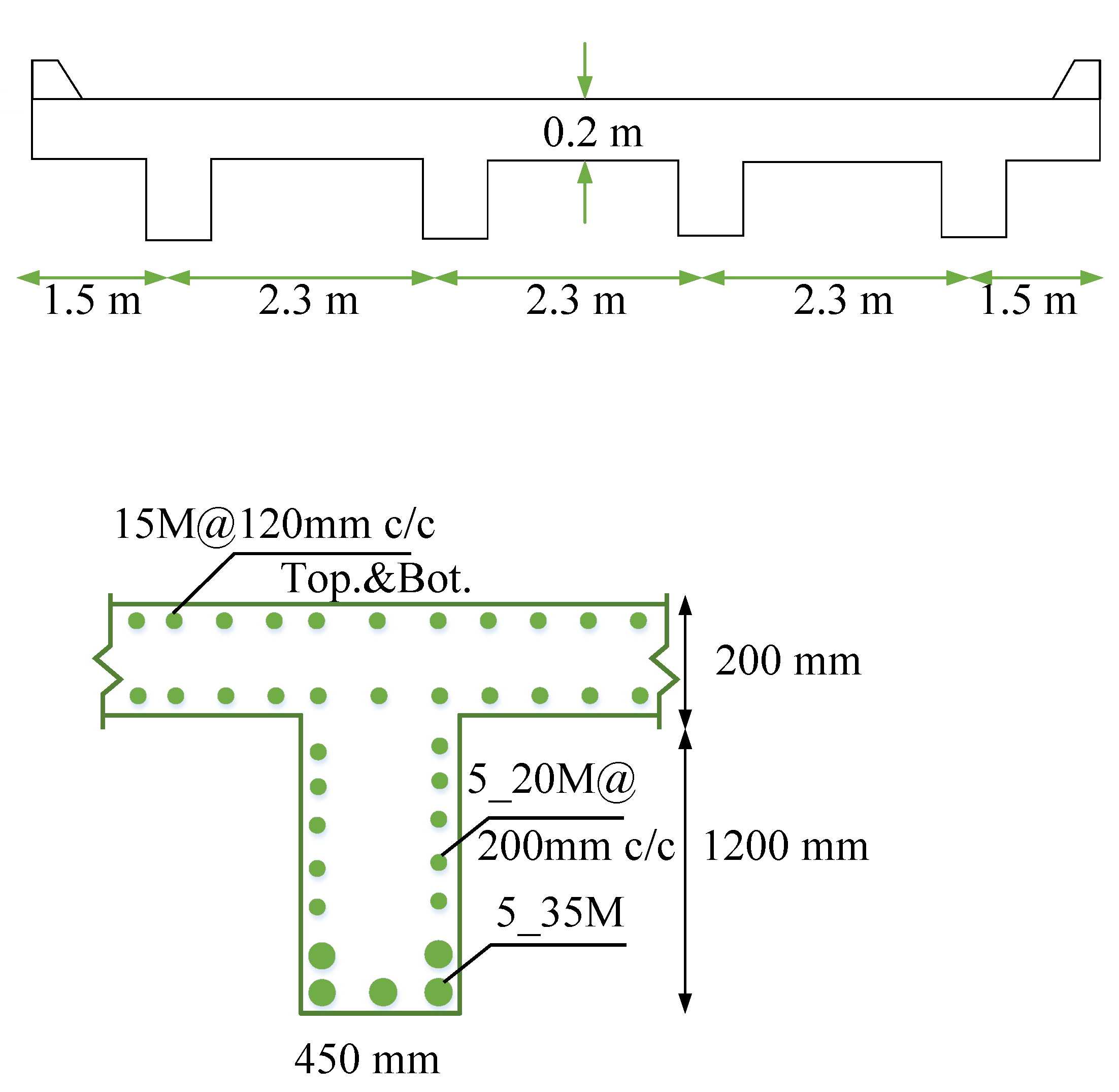
Importantly, the methodology developed is adaptable and can be employed across a diverse array of both traditional and innovative structural systems. The bridge superstructure examined in this case study, as depicted in Figure 2, has an 18 m span (measured from the center of the bearings) and comprises four simply supported reinforced concrete beams that support a slab with a thickness of 0.2 m. The T-section concrete beams are positioned 2.3 m apart, featuring a nominal concrete cover of 60 mm, thereby fulfilling the stipulations of CHBDC-S6.

Furthermore, four diaphragms of concrete are strategically positioned at conclusions and at quarter points along the 18 m span on sides in the transverse direction. The overall space of the bridge superstructure measures 514.5 m², which encompasses deicing materials. Given the scarcity of data related to intervention costs, this study utilizes unit repair costs for composite bridge superstructures as documented in the literature, specifically in Figure 6 [24].

This approach facilitates a more thorough examination of the deterioration and optimization models while also establishing a framework for comparison with prior research. The choice of this particular case study bridge superstructure serves as a realistic and representative instance for applying the established optimization models and deterioration.

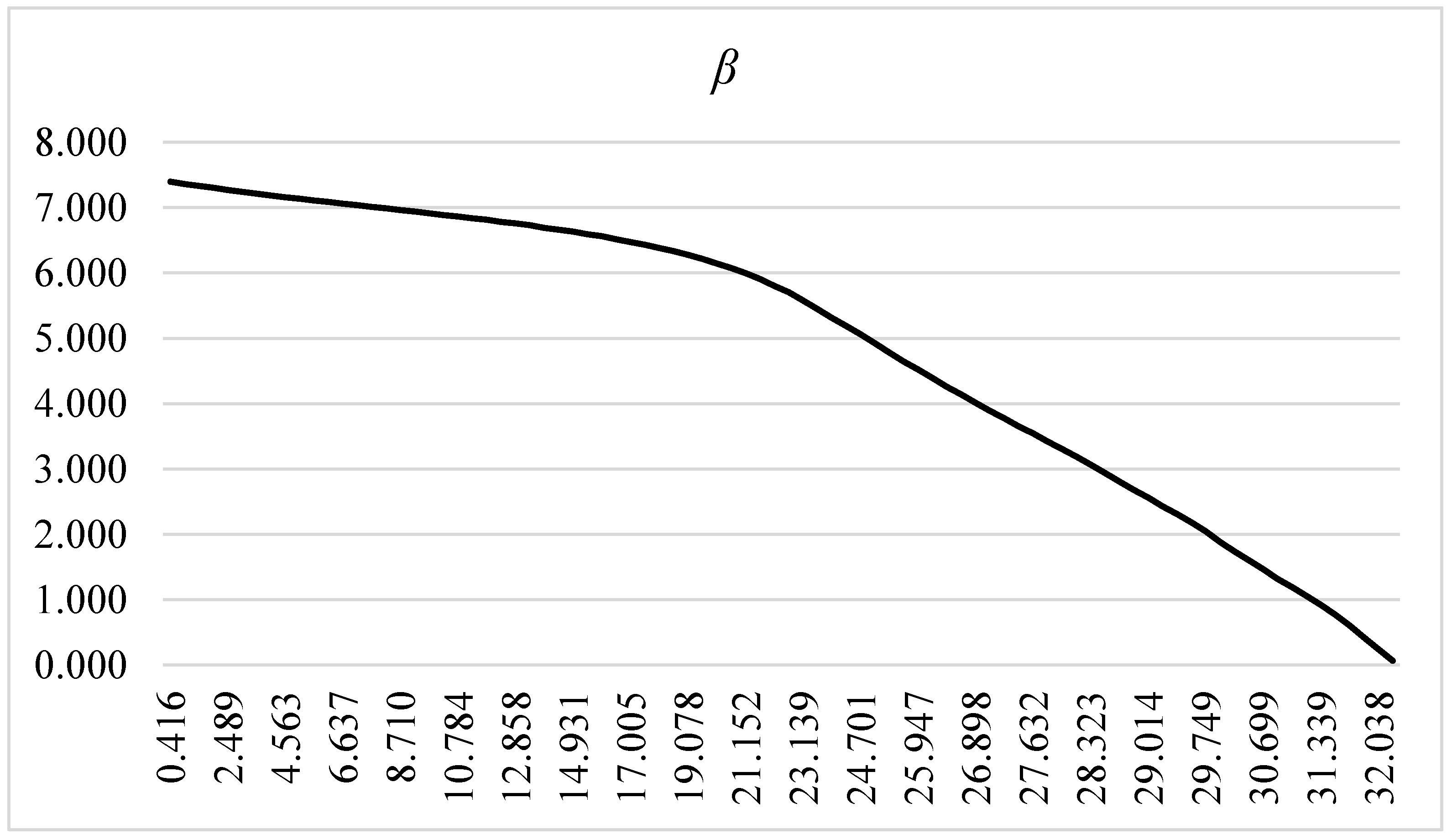
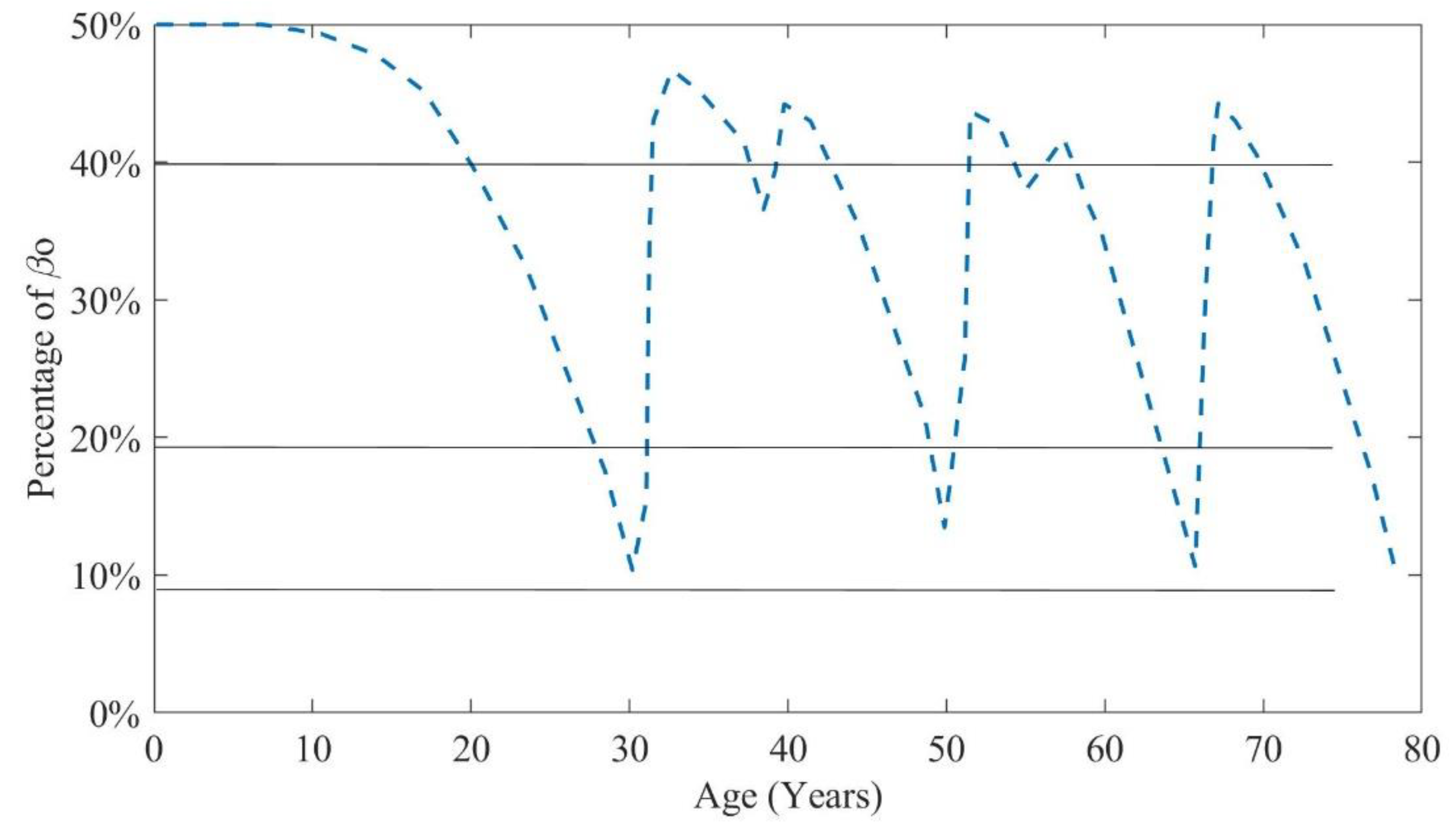
This research examines the degradation pattern of a reinforced concrete superstructure of a bridge situated in a cold space characterized by a severe corrosive environment. The biquadratic curve of degradation, depicted in Figure 7, indicates that the superstructure experiences rapid deterioration when any intervention measures are absent. To determine the most cost-effective intervention strategy, multiple combinations of both major and minor interventions were analyzed. An optimization model was employed to assess the efficacy of each scenario, ensuring compliance with all necessary requirements.

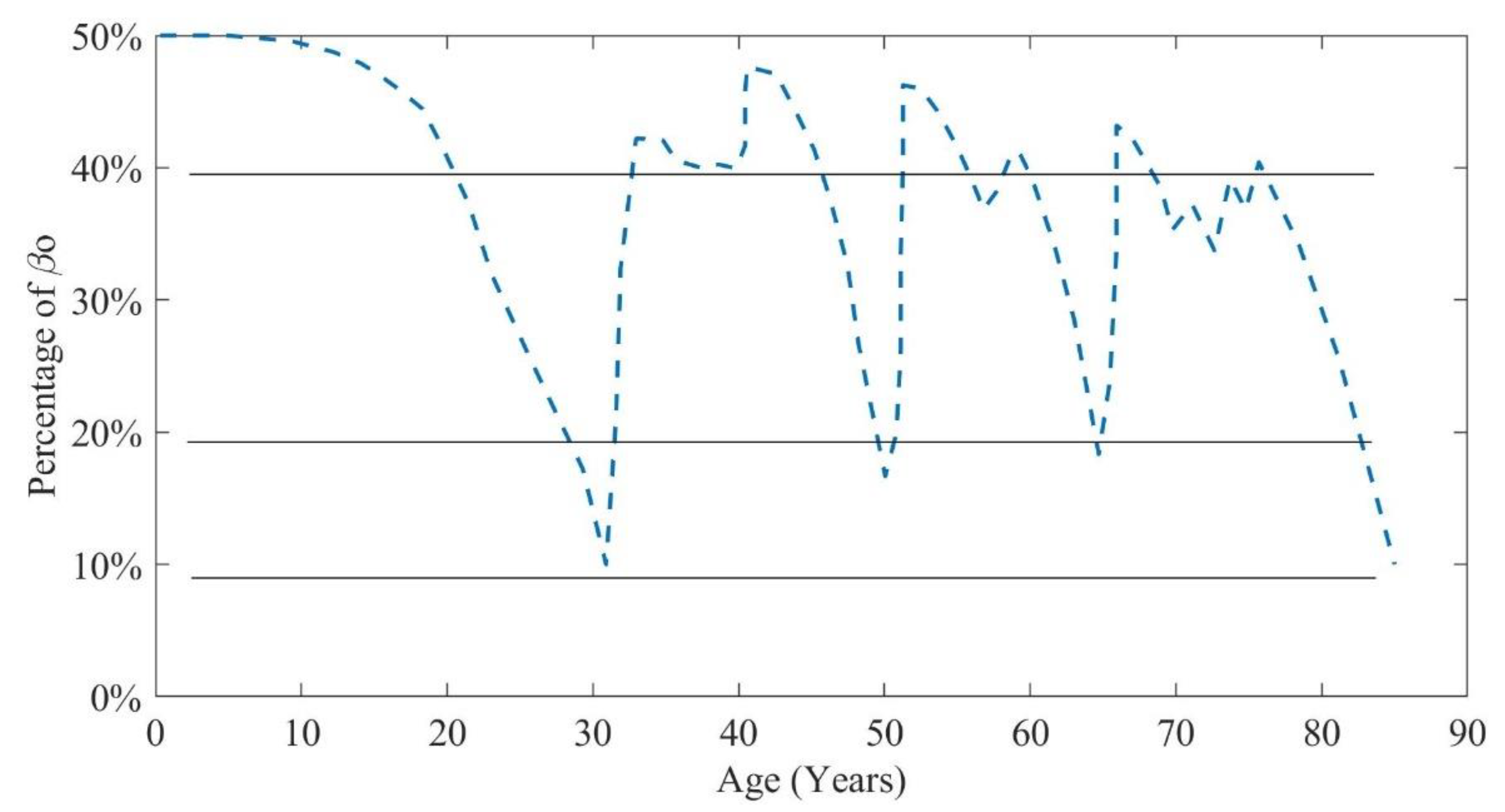
Figure 8 shows a total of three major intervention activities and six minor intervention activities.

The degradation pattern of this scenario is shown in Figure 8, indicating that the reliability index reaches the 0.2 β₀ threshold at Year 85, indicating a perilous circumstance or the termination of the lifecycle of superstructure. The cash flow of this scenario is presented in Figure 9, with an estimated $W_{EUA}$ of USD 12,245 per year.

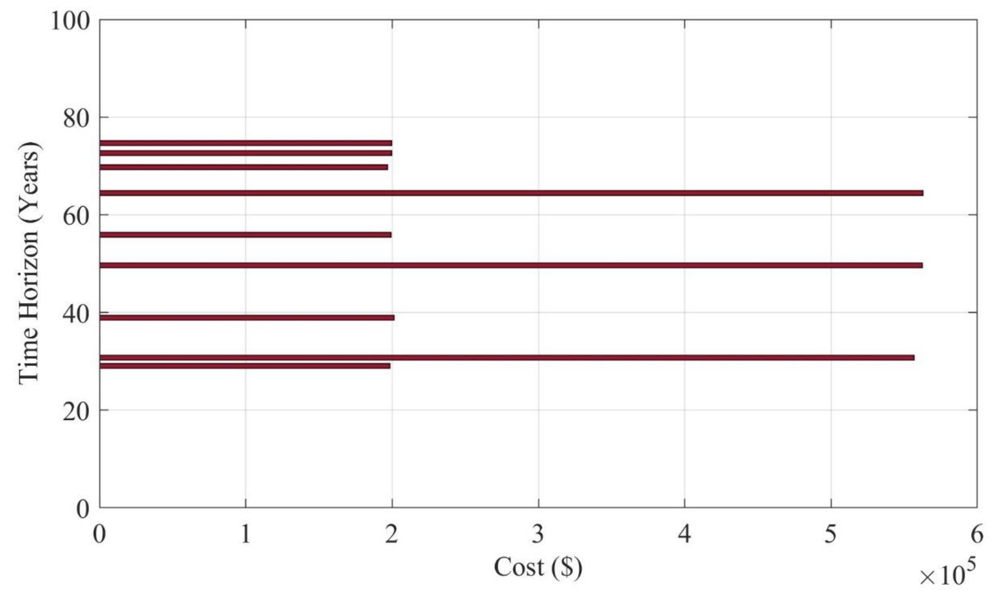
The optimization model selected three chief activities of intervention at Years 65, 50, and 31, along with six minor interventions at Years 31, 38, 58, 63, 72, and 74. The results indicate that the aging process significantly impacts the rate of deterioration, with the interval between chief interventions decreasing over time.

To exemplify, the initial chief intervention is conducted after 30 years, followed by the second after 20 years, and the third after 15 years, confirming the detrimental effect of aging on the deterioration rate. The optimization process revealed that the most economical solution involves two minor interventions and three major interventions, as presented in Figure 10.

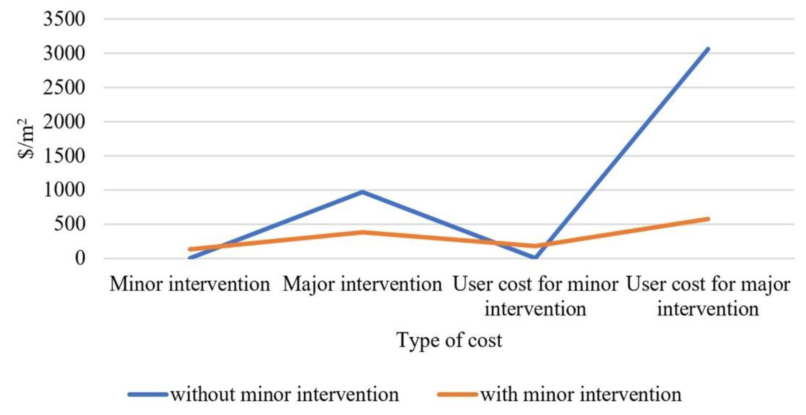
This scenario yields a bridge lifecycle of 79 years with a corresponding $W_{EUA}$ of USD 7624 per year, making it the most cost-effective solution. The results of the optimization process were compared with various scenarios, including the conventional method with no minor interventions, as shown in Figure 11.

The absence of minor interventions significantly increases the overall lifecycle costs and $W_{EUA}$. The highest $W_{EUA}$ of USD 35,438 per year corresponds to the conventional method, which has a service lifecycle of 79 years.

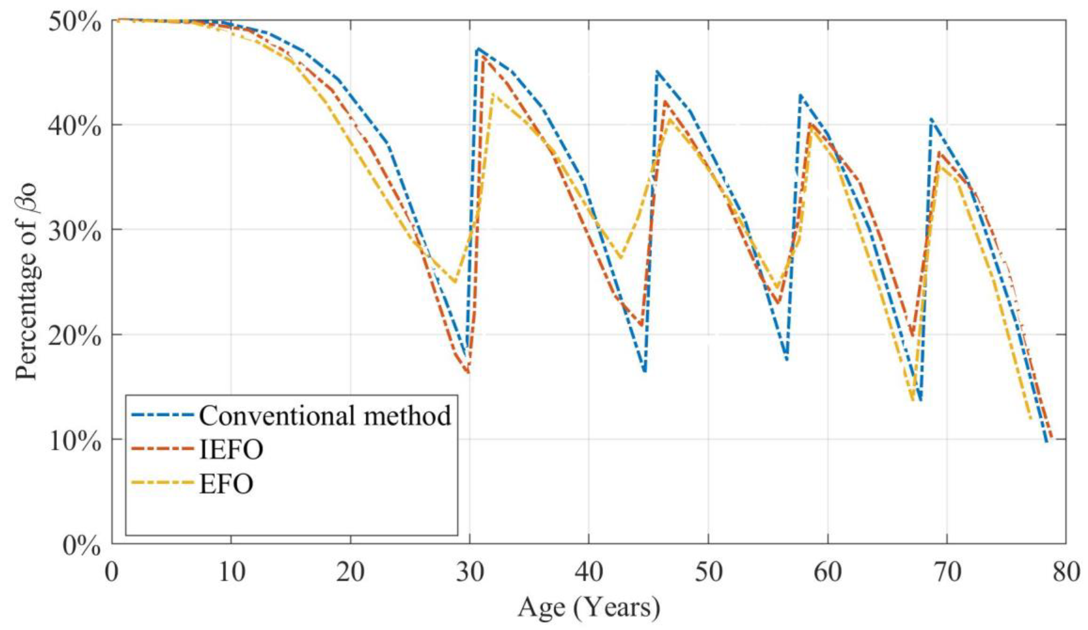
A comparative examination of the deterioration trends based on the proposed IEFO, original EFO, and conventional scenarios revealed a remarkable similarity up to Year 40, as depicted in Figure 12.

However, after this period, the optimal scenario shows a significant enhancement in structural performance, which can be attributed to the strategic application of minor interventions. These interventions, while appearing trivial, have a substantial influence on the overall condition of the bridge, as demonstrated by the improved performance of the optimal scenario.

To show the effectiveness of the FE model, its results were validated based on some results. The first validation was validation with the analytical results. In the table presented above, a comparison was made between the analytical results and those obtained from the Finite Element (FE) model for various beam types. The error was determined by considering the difference between the analytical result and the FE model result, and then dividing this difference by the analytical result.

Table 4. Analytical results of the FE model.

Case	Analytical Result	FE Model Result	Error
Simply Supported Beam	0.012 m	0.0119 m	0.83%
Cantilever Beam	0.025 m	0.0249 m	0.40%
Fixed–Fixed Beam	0.015 m	0.0149 m	0.67%

illustrates the analytical results of the FE model.

The results obtained from the Finite Element (FE) model closely align with the analytical outcomes across all three scenarios, exhibiting an average error of 0.63%. This demonstrates a significant level of precision in forecasting beam deflection under various boundary conditions. Although the error is most pronounced in the simply supported beam scenario at 0.83% and least pronounced in the cantilever beam scenario at 0.40%, the overall findings indicate that the FE model serves as a dependable instrument for this analysis, with only minor variations in accuracy across the different cases.

The experimental findings were contrasted with the results of the Finite Element (FE) model for various beam types. The error was determined by calculating the difference between the experimental result and the FE model result, and then dividing this difference by the experimental result.

Table 5. Validation with experimental results.

Case	Experimental Result	FE Model Result	Error
Reinforced Concrete Beam	0.020 m	0.0198 m	1.00%
Steel Beam	0.015 m	0.0149 m	0.67%
Composite Beam	0.025 m	0.0249 m	0.40%

illustrates the validation with experimental results.

The results obtained from the Finite Element (FE) model closely align with the experimental findings across all three scenarios, exhibiting an average error of 0.69%. This indicates the model’s effectiveness in accurately predicting beam deflection under varying material properties. While there are minor fluctuations in the error rates among the different cases, the reinforced concrete beam scenario shows the greatest deviation, with an error of 1.00%. Conversely, the composite beam scenario demonstrates the least error, recorded at 0.40%. Overall, these findings suggest that the FE model serves as a dependable instrument for conducting such analyses.

The next part of validation here is convergence study. This validation was performed by the outcomes of the Finite Element model and were presented for various mesh sizes.

Table 6. Convergence study.

Mesh Size	Deflection	Stress
0.1 m	0.0199 m	150 Mpa
0.05 m	0.0198 m	149 Mpa
0.01 m	0.0197 m	148 Mpa

indicates the convergence results.

The deflection and stress values in the FE model converged to a stable solution as the mesh size decreased, indicating that the model’s accuracy improved with a finer mesh. Specifically, decreasing the mesh size from 0.1 m to 0.05 m resulted in a reduction of 0.1% in the deflection value and a more significant decrease of 0.67% in the stress value, suggesting that a mesh size of 0.1 m was sufficient for achieving a stable solution, as further refinement yielded only marginal improvements. The deflection and stress values were determined for each mesh size, and the results indicate that the Finite Element model reached a stable solution when a mesh size of 0.1 m was utilized.

The table presented above illustrates the outcomes of the Finite Element (FE) model for various values of Young’s modulus and Poisson ratio.

Table 7. Sensitivity analysis.

Parameter	Deflection	Stress
Young’s Modulus	0.0199 m (30 GPa)	150 MPa
	0.0195 m (25 GPa)	145 MPa
	0.0191 m (20 GPa)	140 MPa
Poisson’s Ratio	0.0199 m (0.2)	150 MPa
	0.0196 m (0.15)	148 MPa
	0.0193 m (0.1)	145 MPa

illustrates the sensitivity analysis.

The findings of the Finite Element (FE) model reveal that the outcomes of deflection and stress were highly dependent on the Young’s modulus value. This suggests that the material characteristics of both the concrete and reinforcement play a crucial role in the model’s forecasts. Specifically, a reduction in Young’s modulus from 30 GPa to 20 GPa resulted in a significant decline in both deflection and stress measurements, with deflection decreasing by 2.5% and stress diminishing by 6.67%. This underscores the necessity of precise characterization of material properties to ensure the reliability of results derived from the FE model.

For each parameter value, the deflection and stress values were computed, revealing that the FE model exhibits sensitivity to the material characteristics of both the concrete and reinforcement.

For validating measures of deterioration and intervention effect models, the deterioration model was validated by the following measures:

-

Mean Absolute Error (MAE): Calculate the MAE between the predicted and actual deterioration values to evaluate the accuracy of the model.

-

Root Mean Square Error (RMSE): Calculate the RMSE between the predicted and actual deterioration values to evaluate the accuracy of the model.

-

Coefficient of Determination (R-squared): Calculate the R-squared value to evaluate the goodness of fit of the model.

Table 8. Deterioration model’s validation metrics.

Metric	Value
MAE	0.05
RMSE	0.10
R-squared	0.80

indicates the deterioration model’s validation metrics.

The results presented in Table 8 indicate that the deterioration model demonstrated a considerable level of accuracy, evidenced by a Mean Absolute Error (MAE) of 0.05 and a Root Mean Square Error (RMSE) of 0.10. Furthermore, the R-squared value of 0.80 suggests that the model effectively accounted for a substantial portion of the variability within the dataset.

6. Discussions

The proposed framework can be adapted for various types of substructures, including tunnels and roads, through specific modifications. This process entails identifying the distinct characteristics associated with each infrastructure type, such as geometry, materials, loads, and the requirements for analysis and simulation. For tunnels, adjustments would be necessary in the geometric modeling aspect to reflect the unique shape and dimensions of tunnel cross-sections, as well as in the material modeling to incorporate the specific materials utilized in tunnel construction, including concrete, steel, and rock. Furthermore, the load modeling component must be revised to consider the particular loads that tunnels experience, such as soil pressure, water pressure, and traffic loads. The analysis and simulation component would also require modifications to address the specific needs of tunnels, including soil–structure interaction analysis and the simulation of tunnel excavation and construction processes. In a similar vein, for roads, the geometric modeling would need to be adjusted to represent the unique geometry of road cross-sections, while the material modeling would have to account for the specific materials employed in road construction, such as asphalt, concrete, and aggregate.

The load modeling component must be adjusted to reflect the particular loads that roads encounter, including traffic loads, wind loads, and temperature loads. Additionally, the analysis and simulation component should be revised to meet the unique analysis and simulation needs of roads, such as examining pavement–vehicle interaction and simulating road traffic. By broadening the framework in this manner, it can be used for a greater variety of infrastructure types, thereby enhancing its applicability, utility, accuracy, and reliability. However, this expansion may also elevate the complexity of the framework, necessitating more comprehensive validation and testing.

The proposed framework presents also has limitations that warrant careful consideration. These include the reliance on assumptions of linear relationships and normal data distributions, the oversimplification of intricate relationships, and the constraints imposed by limited data requirements. Furthermore, the complexity of the model raises interpretability challenges, while scalability issues may arise when dealing with large datasets or complex problems. The framework also lacks the incorporation of domain knowledge, poses risks of overfitting, and demonstrates insufficient robustness to variations in inputs or outputs. Such limitations could adversely affect the framework’s performance and accuracy, especially if the underlying assumptions are not met if the data are limited or contain noise, or if the model lacks interpretability. Additionally, the framework’s scalability and robustness may be endangered if the computational demands, in terms of time and memory, are excessive or if there are fluctuations in inputs or outputs over time.

7. Conclusions

The aging and degradation of bridge structures present considerable challenges for asset managers, who must identify the necessity of maintenance against constrained financial resources. Conventional maintenance approaches typically emphasize reactive repairs, which can result in elevated lifecycle expenses and risk structural integrity. To address these problems, this research required establishing an innovative framework aimed at optimizing bridge maintenance expenditures while maintaining structural safety. The proposed methodology incorporates a reliability-based deterioration model, an intervention effect model, a financial model, and an optimization model empowered by an Improved Electric Fish Optimization (IEFO) algorithm. This framework was tested through a case study involving a fundamentally supported superstructure of a bridge constructed based on the design standards of the Canadian highway bridge. The outcomes of this investigation highlighted the efficacy of the proposed methodology in reducing lifecycle costs while ensuring structural safety. The deterioration model exhibited a commendable level of precision, achieving a Mean Absolute Error (MAE) of 0.05 and a Root Mean Square Error (RMSE) of 0.10, along with an R-squared value of 0.80. This indicates that the model successfully achieved a significant portion of the variability present in the dataset. The optimization model pinpointed the most cost-efficient intervention strategy, which comprises three primary intervention activities scheduled for Years 65, 50, and 31, along with six secondary interventions planned for Years 31, 38, 58, 63, 72, and 74. The aging process notably influences the deterioration rate, leading to a reduction in the intervals between primary interventions over time. The most cost-effective approach, which includes two minor and three major interventions, resulted in a bridge lifecycle of 79 years, with a corresponding Whole-Life Equivalent Uniform Annual Worth ($W_{EUA}$) of USD 7624 annually. In contrast, the omission of minor interventions significantly escalated the overall lifecycle costs and $W_{EUA}$, with the conventional method yielding the highest $W_{EUA}$ of USD 35,438 per year. Furthermore, the Finite Element (FE) model reached a stable solution as the mesh size was reduced, with a mesh size of 0.1 m deemed adequate for stability. The model also demonstrated sensitivity to the material properties of both the concrete and reinforcement, where a decrease in Young’s modulus from 30 GPa to 20 GPa led to a notable reduction in both deflection and stress measurements. The IEFO algorithm successfully identified the most economically viable maintenance strategies, including minor repairs that could postpone the necessity for expensive major interventions. The optimal scenario determined by the IEFO engine yielded lower equivalent uniform annual costs in comparison with the traditional scenario focused solely on major repairs. Future research can build on this study by exploring the application of the proposed framework to other infrastructure assets and investigating the integration of additional factors, such as environmental and social impacts, into the optimization process.