

Study on Compression Bearing Capacity of Tapered Concrete-Filled Double-Skin Steel Tubular Members Based on Heuristic-Algorithm-Optimized Backpropagation Neural Network Model

 ,
, 

Abstract
1. Introduction
2. Testing Database
2.1. Experiment Database
2.2. Finite Element Database

2.3. Database Processing
3. Prediction of Axial Compressive Capacity Based on BPNN
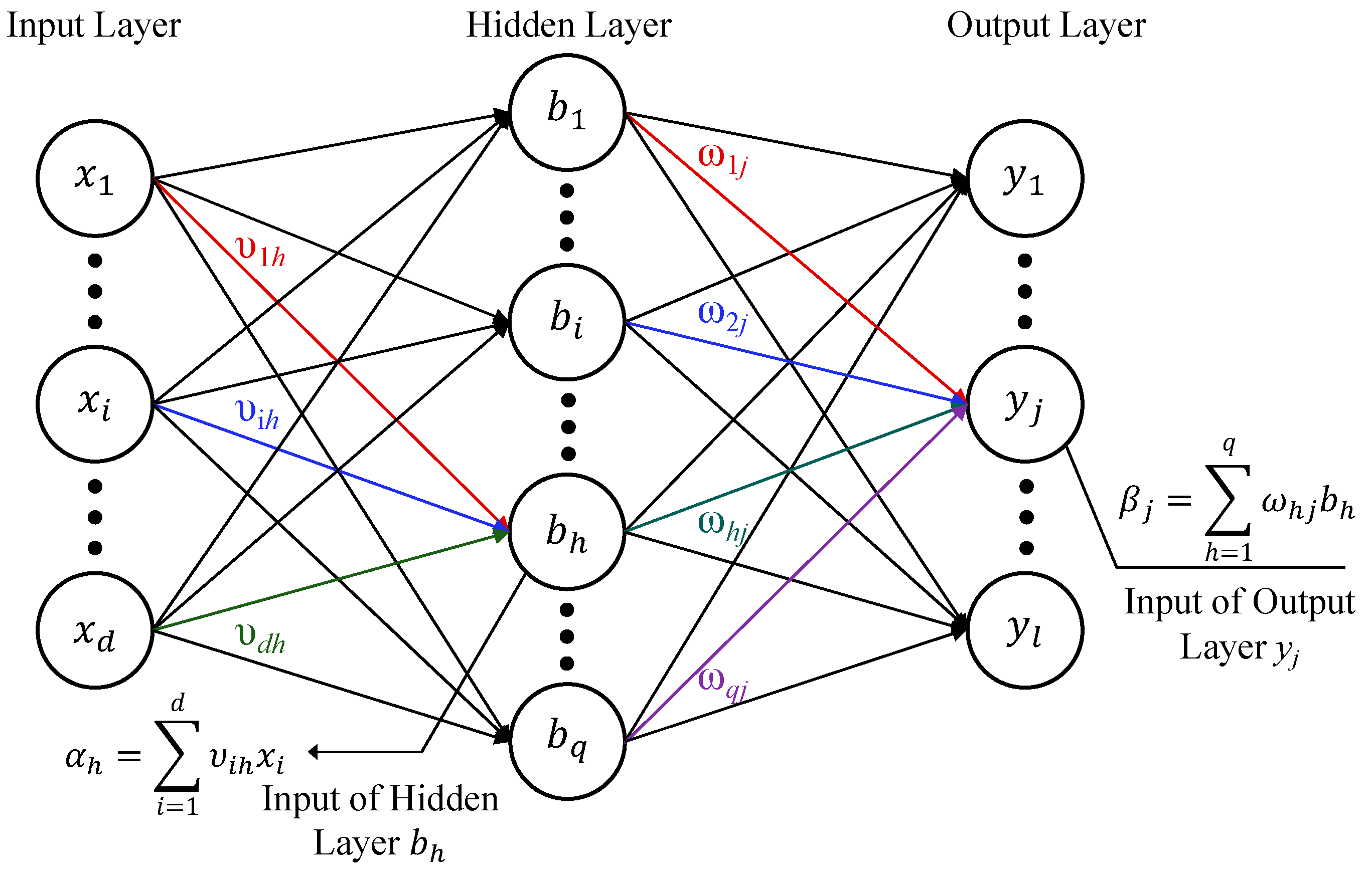
3.1. Standard BP Neural Network
3.2. Optimizing BPNN with Genetic Algorithm (GA-BPNN)
3.2.1. Advantages and Specific Contributions of GA
- (1)
- Global exploration: GA maintains a diverse population of solutions, encouraging exploration and preventing premature convergence.
- (2)
- Robustness to nonlinear surfaces: GA operates independently of gradient information, making it suitable for handling the complex, nonlinear error surfaces typically associated with BPNN.
- (3)
- Crossover and mutation: These genetic operations allow GA to combine and alter solutions, promoting diversity in the search space.
- (4)
- Role in optimization: GA is particularly effective in the initial stages of optimization, where broad exploration of the solution space is essential. By simulating evolutionary processes, GA efficiently identifies promising regions in the search space, balancing exploration and exploitation of the network weights and thresholds.
3.2.2. Detailed Steps for Optimizing BPNN Using GA
- (1)
- The optimization process for the GA-BPNN begins with the initialization of the population, where random weights and thresholds for the BPNN are generated as chromosomes. Each chromosome represents a potential solution with encoded weights and thresholds. The BPNN is then trained using these initial weights, and the Root Mean Square Error (RMSE) is calculated between the predicted and actual values. Based on this RMSE, the fitness of each chromosome is evaluated. If the error does not meet the precision requirements, the Genetic Algorithm (GA) is applied to optimize the weights and thresholds.
- (2)
- During the GA process, parameters such as selection rate, crossover probability, and mutation rate are set to guide the optimization. The selection rate controls the proportion of individuals chosen to form the next generation, balancing the trade-off between intensifying the search around high-fitness solutions and maintaining population diversity. A higher selection rate favors the exploitation of fitter individuals, while a lower rate preserves genetic diversity. The crossover probability determines the likelihood of combining two parent solutions to explore new areas of the solution space, while the mutation rate introduces random changes to genes (weights and thresholds), preventing premature convergence to local minima. Through these genetic operations, the population is iteratively updated, minimizing RMSE and generating new sets of weights and thresholds. This updated population then serves as the initial population for the next generation.
- (3)
- Once the global optimization through GA achieves the desired accuracy, the process moves into the local optimization phase. The final optimized weights and thresholds from the GA are used as inputs for the BPNN, and the BPNN is employed as a prediction tool (without additional training) to further fine-tune the weights and thresholds. During this phase, GA continues to refine the solution by adjusting the weights and thresholds through additional selection, crossover, and mutation processes. This continues until the RMSE satisfies the predefined accuracy requirements, resulting in the final set of optimized weights, thresholds, and minimal error.
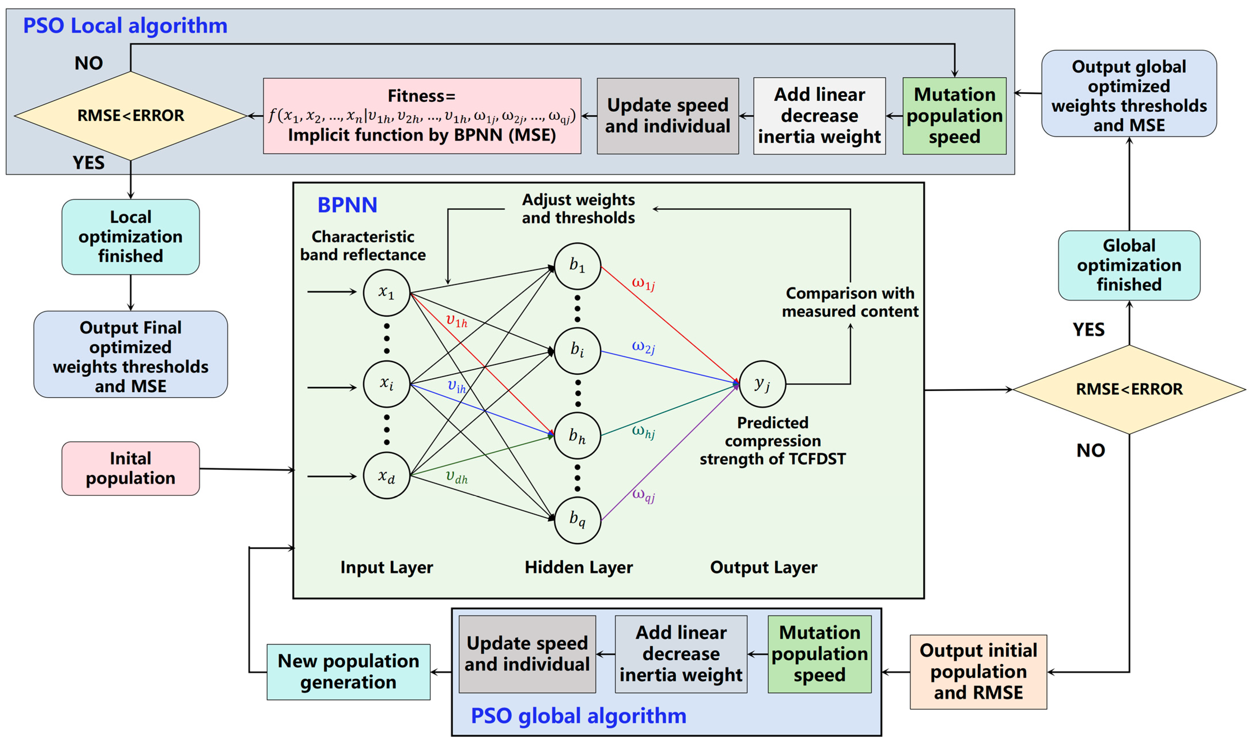
3.3. Optimizing BPNN with Particle Swarm Optimization Algorithm (PSO-BPNN)
3.3.1. Advantages and Specific Contributions of PSO
- (1)
- Balance of exploration and exploitation: PSO strikes a balance between exploration and exploitation by allowing particles to move toward better-known solutions while exploring new areas of the solution space.
- (2)
- Faster convergence: Compared to GA, PSO tends to converge more quickly, as it directly updates the solutions based on the experience of the best particles.
- (3)
- Simplicity: PSO requires fewer parameters to tune, making it simpler to implement and computationally efficient.
3.3.2. Detailed Steps for Optimizing BPNN Using PSO
- (1)
- The optimization process begins with the initialization of the population, where initial weights and thresholds for the BPNN are randomly set. Subsequently, the BPNN is trained, and the Root Mean Square Error (RMSE) between the predicted and actual values is calculated. Based on this error, the algorithm determines whether the error tolerance is met. If the error does not meet the precision requirements, the initial population along with the calculated RMSE is fed into the PSO (Particle Swarm Optimization) algorithm for further optimization.
- (2)
- During the PSO process, parameters such as the inertia weight, cognitive (personal) learning coefficient, and social (global) learning coefficient are set to guide the optimization. The inertia weight controls the impact of the previous velocity on the current velocity, which balances the trade-off between exploration (global search) and exploitation (local search). A higher inertia weight favors exploration, while a lower one favors exploitation. The cognitive coefficient encourages each particle to return to its personal best-known position, while the social coefficient leads the particles towards the global best-known position found by the entire swarm. Through these updates, the particles’ velocities and positions are adjusted iteratively to minimize the RMSE, ultimately generating a new set of weights and thresholds. This updated population is then used as the initial population for the next generation.
- (3)
- Once the global optimization reaches the desired accuracy, the process transitions into the local optimization phase. The final optimized weights and thresholds from the global optimization step are used as inputs for the PSO algorithm, with BPNN functioning as a prediction tool in this stage (no additional training is performed). The net generated by BPNN, viewed as a function, is continuously fine-tuned by PSO to further optimize the weights and thresholds. This iterative process continues until the RMSE meets the predefined precision requirement, yielding the final set of weights, thresholds, and RMSE that minimizes the error between predicted and actual values.
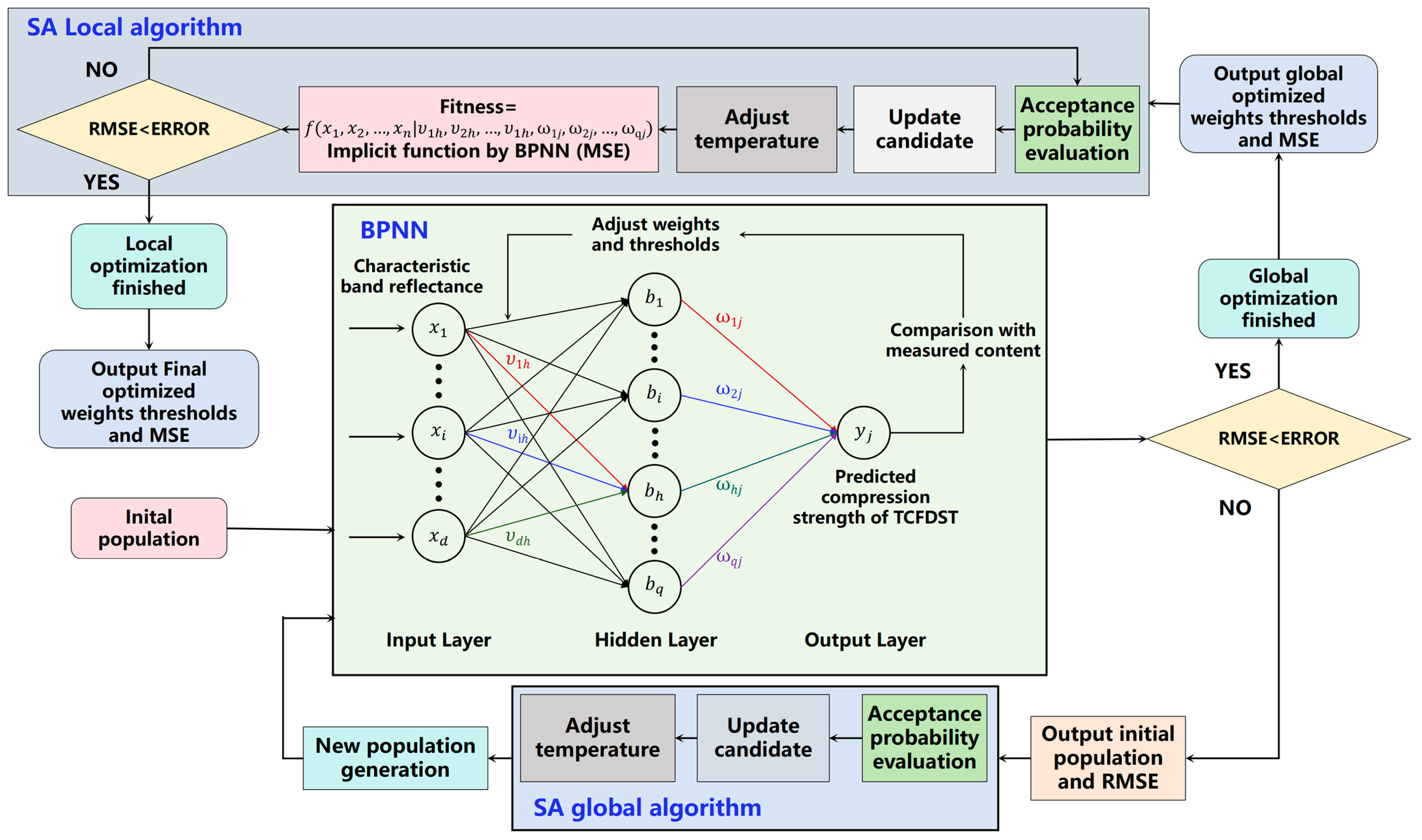
3.4. Optimizing BPNN with Simulated Annealing Algorithm (SA-BPNN)
3.4.1. Advantages and Specific Contributions of SA
- (1)
- Escaping local optima: SA’s acceptance of worse solutions early in the process allows it to escape local minima, an important feature when optimizing complex error surfaces like those in BPNN.
- (2)
- Gradual refinement: SA reduces the probability of accepting worse solutions as the algorithm progresses, allowing it to transition from exploration to exploitation.
- (3)
- Simplicity: SA is relatively easy to implement and requires minimal parameter adjustments.
- (4)
- Role in optimization: SA is well suited for fine-tuning weights and thresholds; its ability to escape local minima makes it a robust tool for refining solutions and ensuring that the final weights and thresholds are near-optimal.
3.4.2. Detailed Steps for Optimizing BPNN Using SA
- (1)
- The optimization process begins with the initialization of weights and thresholds for the BPNN, which are set randomly. The BPNN is then trained, and the Root Mean Square Error (RMSE) between the predicted and actual values is calculated. If the error does not meet the predefined precision requirements, the Simulated Annealing (SA) algorithm is applied to optimize the weights and thresholds further.
- (2)
- During the SA process, key parameters such as the initial temperature, cooling schedule, and acceptance probability are defined. The initial temperature controls the likelihood of accepting worse solutions, enabling the algorithm to explore a wider range of potential solutions. As the temperature decreases according to the cooling schedule, the algorithm gradually shifts from exploration to exploitation, focusing more on refining the current solution. The acceptance probability allows the algorithm to occasionally accept solutions with higher RMSE, preventing it from becoming stuck in local minima and encouraging exploration of the solution space. By iteratively perturbing the weights and thresholds and accepting or rejecting changes based on the temperature and acceptance probability, the SA process minimizes RMSE.
- (3)
- Once the global optimization phase reaches the desired accuracy, the process transitions into the local optimization phase. In this stage, the final optimized weights and thresholds from the global optimization step are used as inputs, and BPNN acts as a prediction tool (without further training). The net generated by BPNN is fine-tuned through additional iterations of SA, where further adjustments to the weights and thresholds are made to minimize RMSE further. The iterative process continues until the RMSE satisfies the predefined precision requirement, yielding the final optimized set of weights, thresholds, and RMSE that minimizes the error between the predicted and actual values.
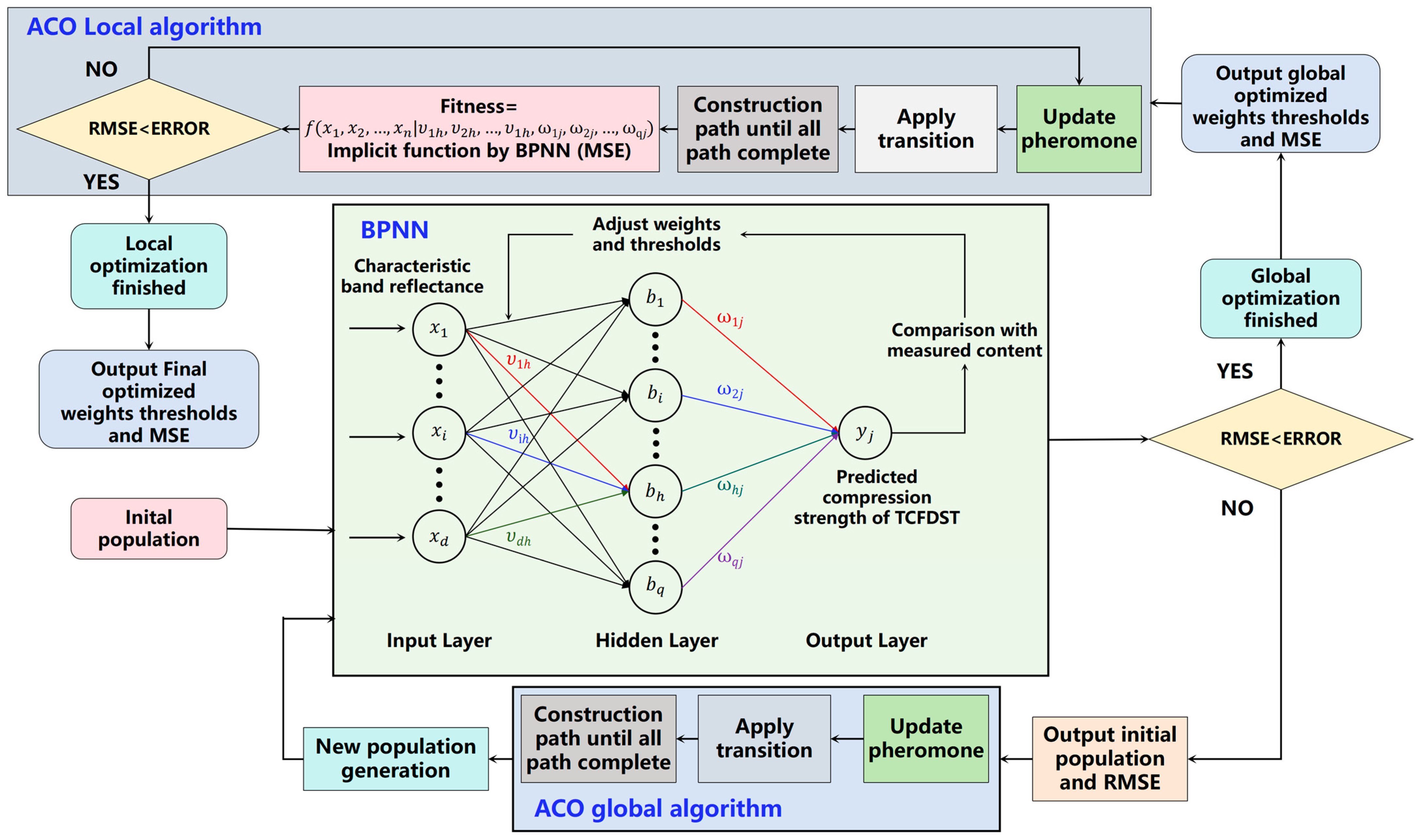
3.5. Optimizing BPNN with Ant Colony Optimization Algorithm (ACO-BPNN)
3.5.1. Advantages and Specific Contributions of ACO
- (1)
- Efficient combinatorial search: ACO excels in solving combinatorial optimization problems and efficiently explores combinations of weights and thresholds in BPNN.
- (2)
- Positive feedback mechanism: Successful solutions increase their selection probability through pheromone updates, guiding the search toward optimal areas in the solution space.
- (3)
- Adaptability: ACO dynamically adjusts its search strategy based on feedback, making it responsive to changes in the optimization landscape.
- (4)
- Role in optimization: ACO is particularly effective for identifying optimal or near-optimal combinations of weights and thresholds in complex, multi-dimensional optimization problems like BPNN. Its iterative refinement helps to focus the search on the most promising solutions.
3.5.2. Detailed Steps for Optimizing BPNN Using ACO
- (1)
- The optimization process begins with the initialization of the population, where the initial weights and thresholds for the BPNN are randomly set. The BPNN is trained using these initial weights, and the Root Mean Square Error (RMSE) between the predicted and actual values is calculated. If the error does not meet the predefined precision requirement, the Ant Colony Optimization (ACO) algorithm is applied to optimize the weights and thresholds further.
- (2)
- During the ACO process, key parameters such as the number of ants, pheromone evaporation rate, and influence of pheromone trails are defined to guide the search for optimal solutions. Ants represent individual solutions (sets of weights and thresholds), and each ant constructs a solution based on probabilistic rules that are influenced by the pheromone trails left by previous solutions and heuristic information. As ants explore the solution space, pheromone is deposited on paths that lead to better solutions (lower RMSE), making those paths more likely to be followed by subsequent ants. A pheromone evaporation rate is applied to prevent the algorithm from converging too quickly to local minima by reducing the influence of older paths. This process continues iteratively as ants adjust their paths (weights and thresholds) to explore the search space effectively, minimizing RMSE.
- (3)
- Once the global optimization through ACO reaches the desired accuracy, the process transitions into the local optimization phase. In this phase, the final optimized weights and thresholds obtained from the global ACO optimization are used as inputs for further fine-tuning. BPNN functions as a prediction tool during this stage (without additional training). The net generated by BPNN is continuously refined through additional iterations of ACO, further optimizing the weights and thresholds until the RMSE satisfies the precision requirement. This iterative process continues until the final set of weights, thresholds, and RMSE is obtained, minimizing the error between predicted and actual values.
3.6. Model Evaluation Metrics
- (1)
- Root Mean Square Error (RMSE): This metric represents the square root of the average of the squares of the differences between predicted and actual values. It is used to measure the variation between the predictions and the actual observations.
- (2)
- Mean Absolute Error (MAE): MAE is the average of the absolute differences between the predicted values and the actual values. It evaluates the degree of deviation in the prediction results.
- (3)
- Mean Absolute Percentage Error (MAPE): MAPE measures the average of the absolute differences between the predicted and actual values divided by the actual values, typically expressed as a percentage. It provides an insight into the prediction accuracy in relative terms.
- (4)
- Coefficient of Determination (R2): R2 indicates the degree of fit between the predicted values and the actual values. A value of R2 lies in the range [0, 1], where 1 indicates perfect prediction accuracy.
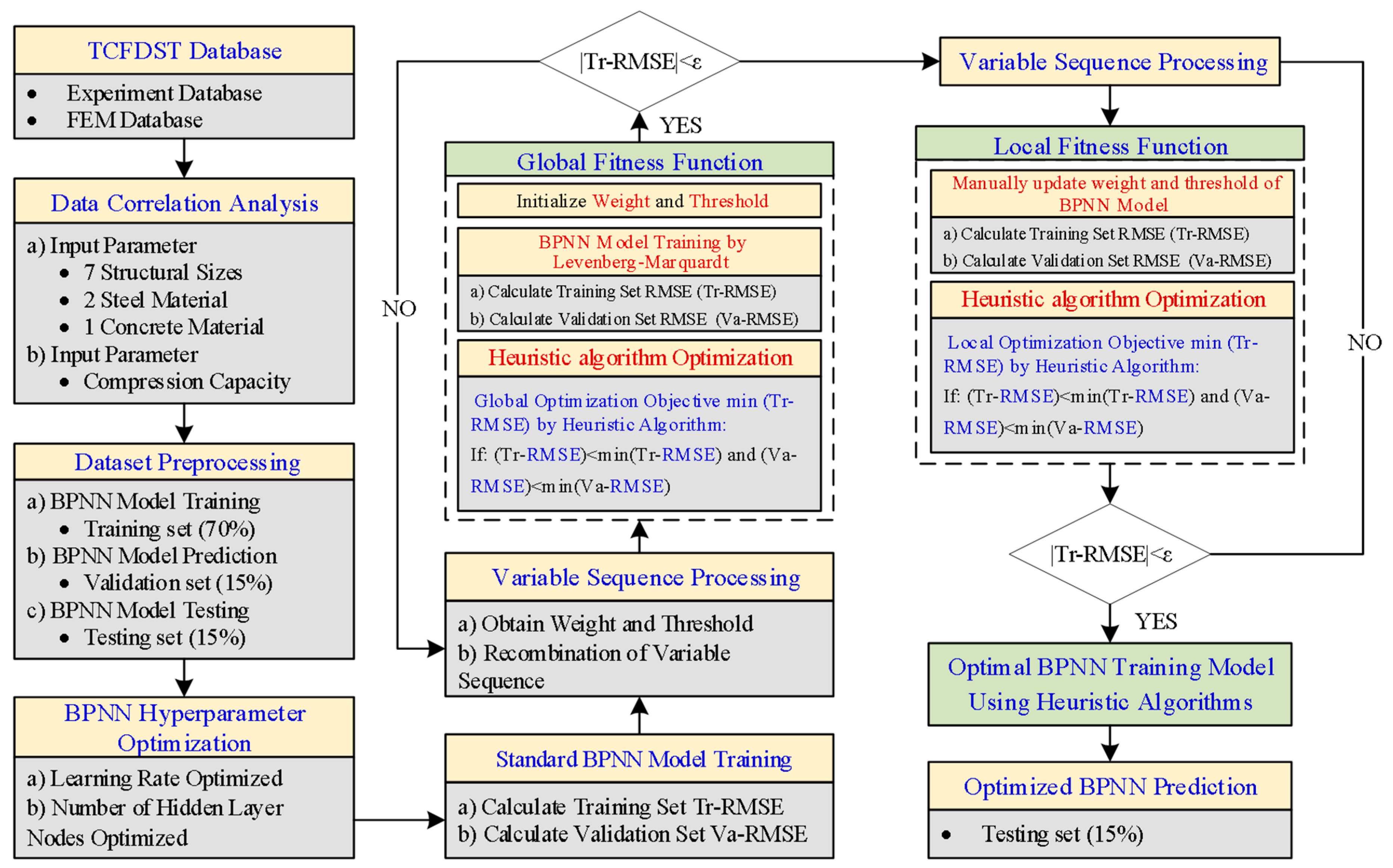
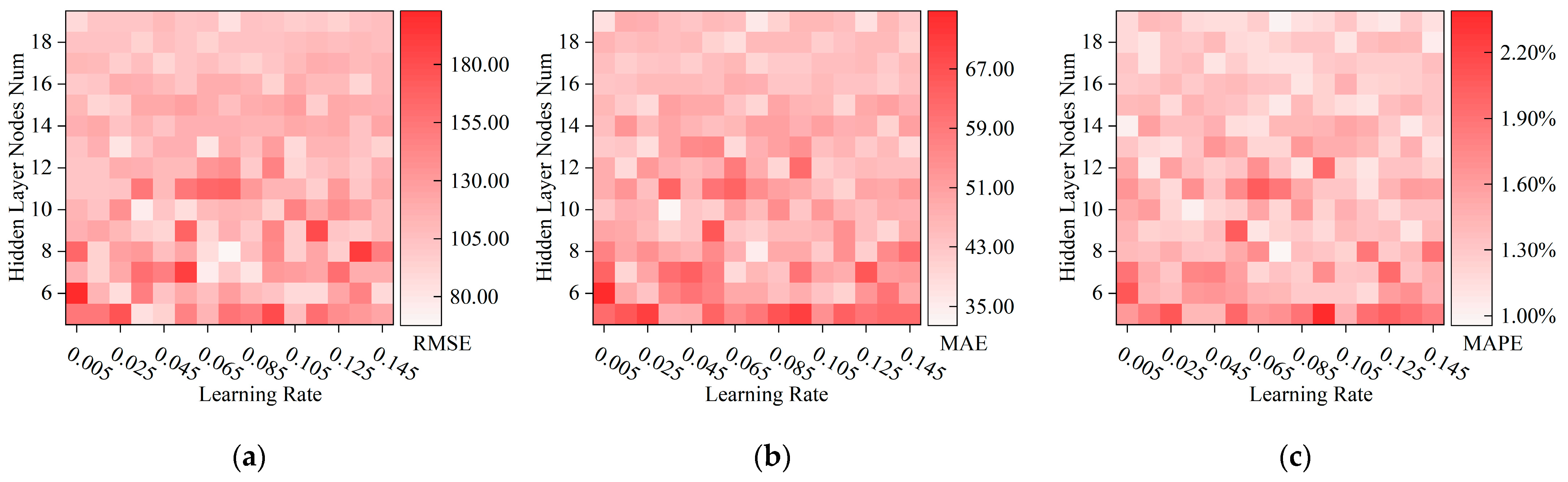
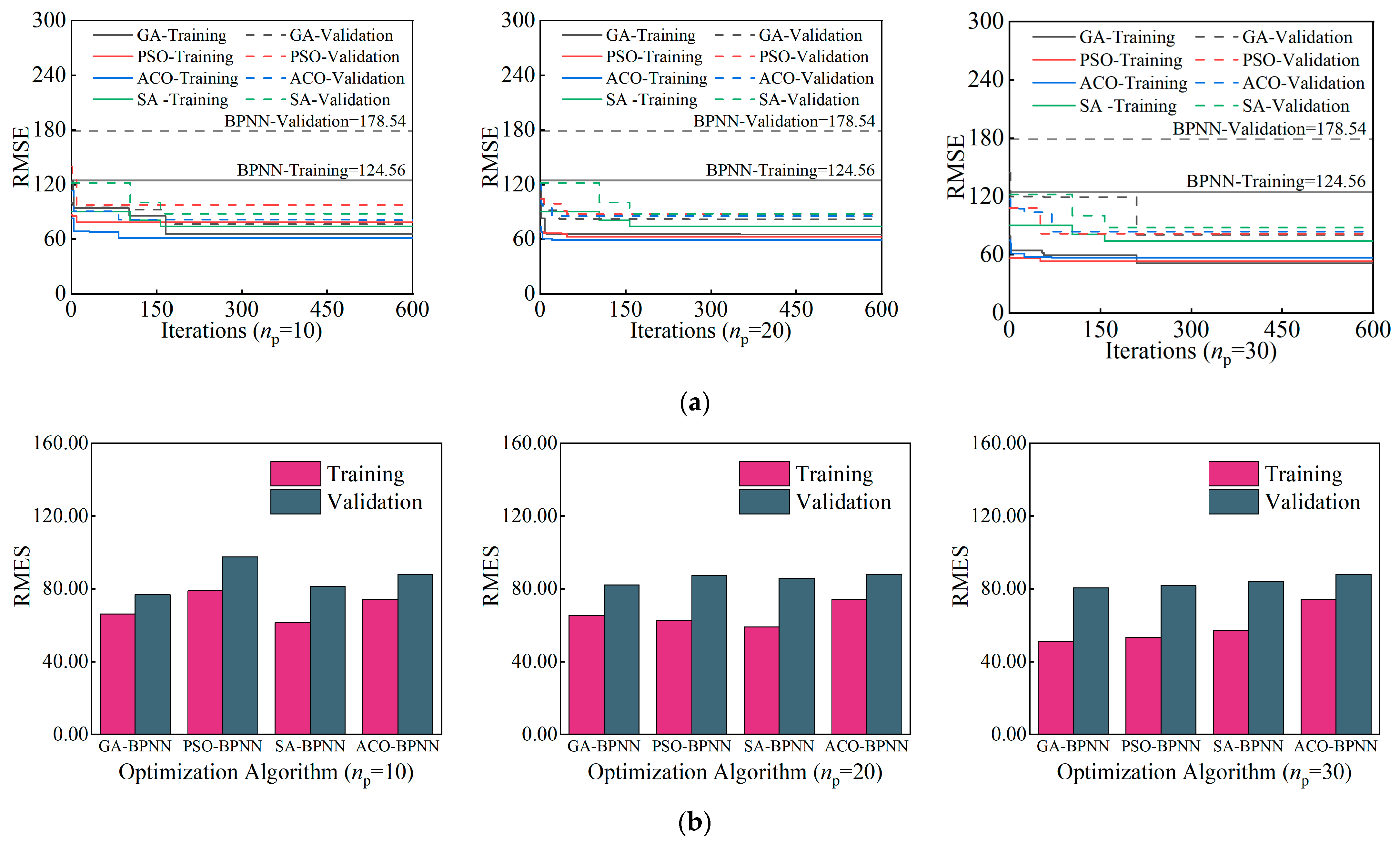
3.7. Hyperparameter Tuning
4. Comparison of Optimization Effects
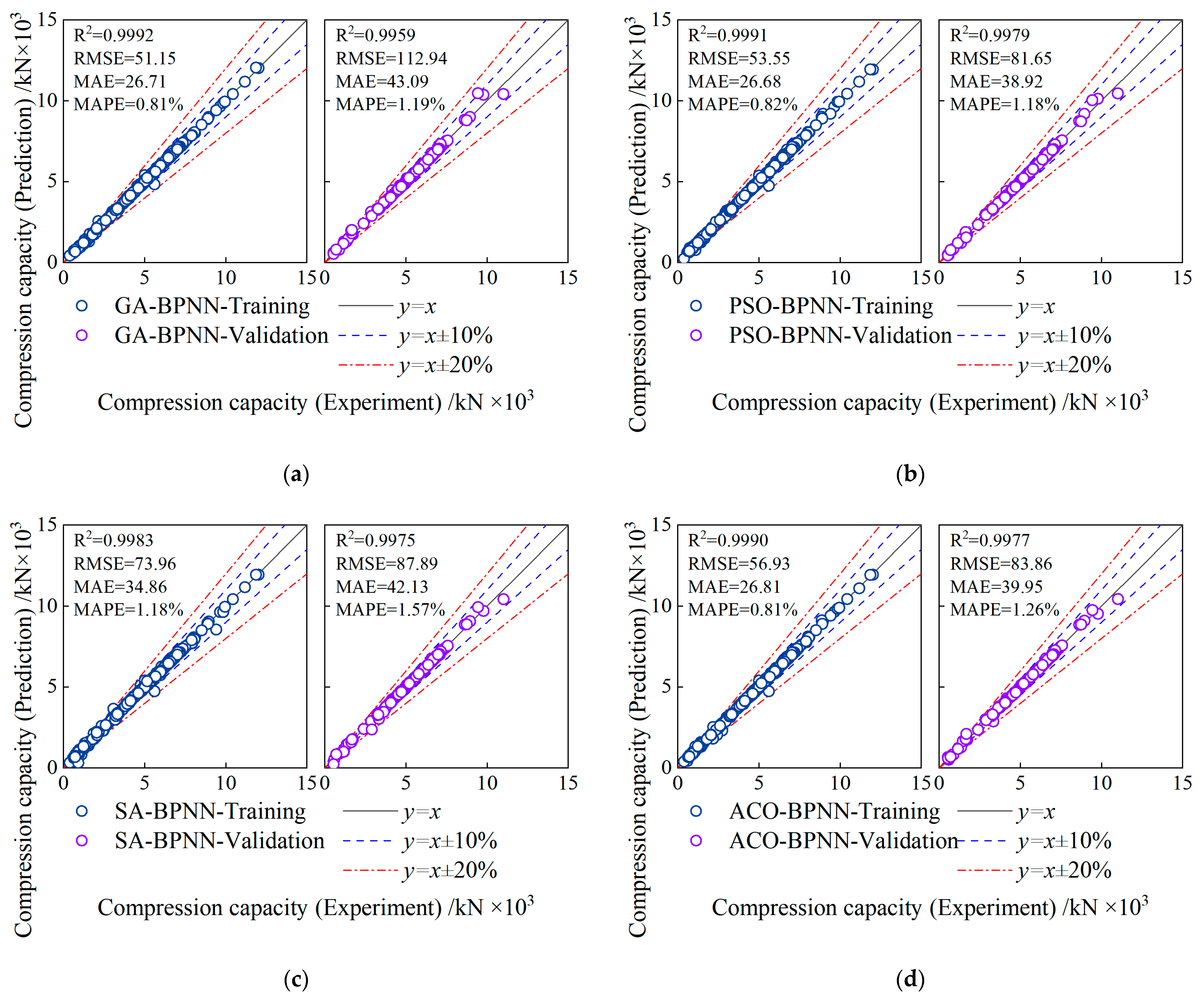
4.1. Comparison of Model Performance Metrics
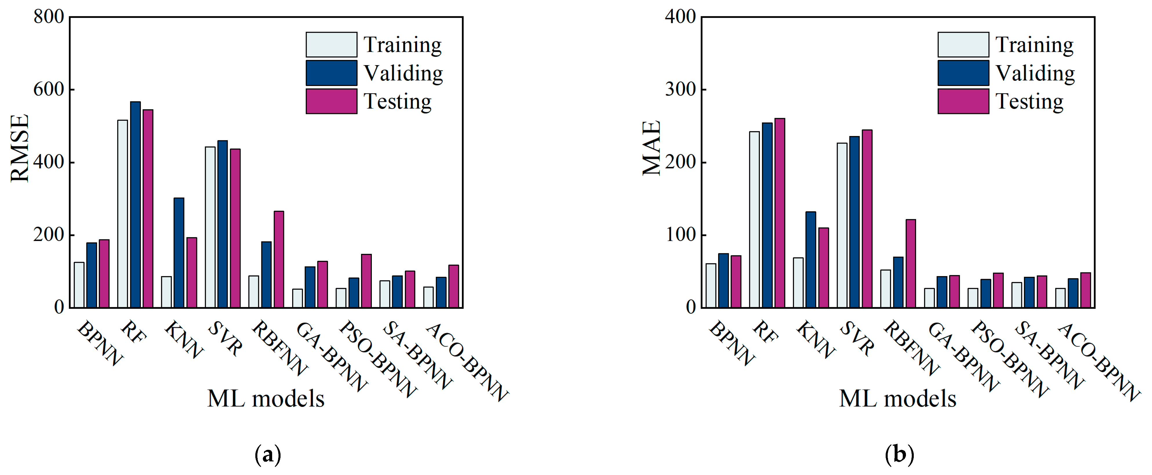
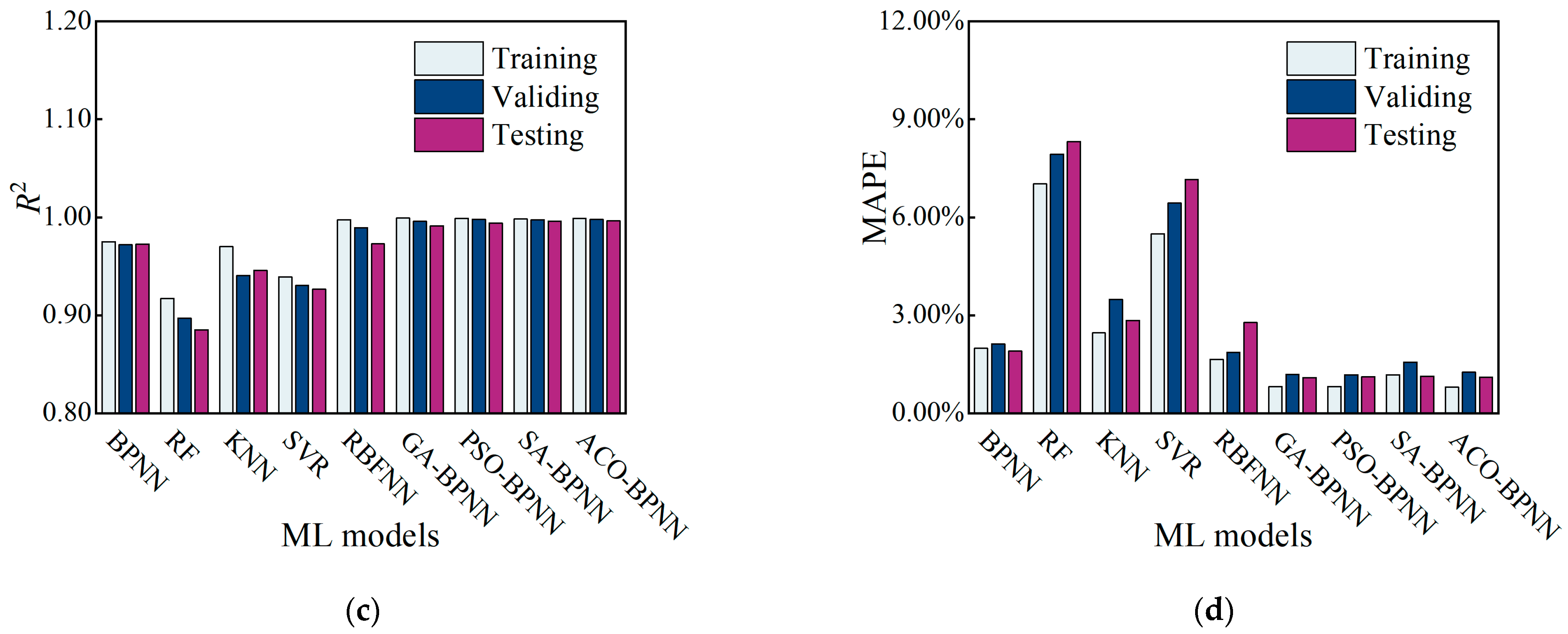
4.2. Comparison of Other Machine Learning Methods
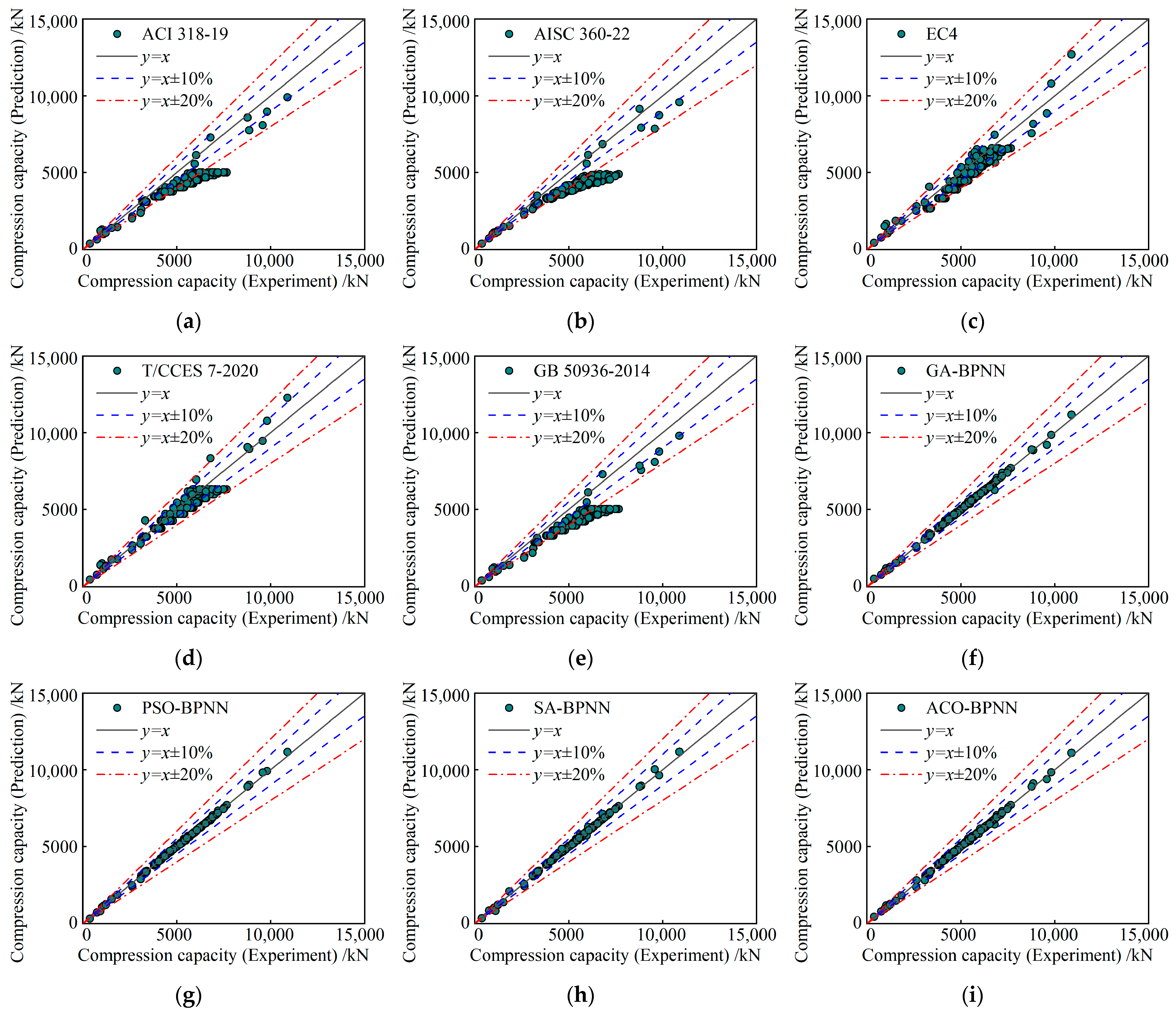
5. Comparison of Design Code Results
5.1. Modified ACI 318-19 Method
5.2. Modified AISC 360-22 Method
5.3. Modified EC4 Method
5.4. T/CCES 7-2020 Method
5.5. Modified GB 50936-2014 Method
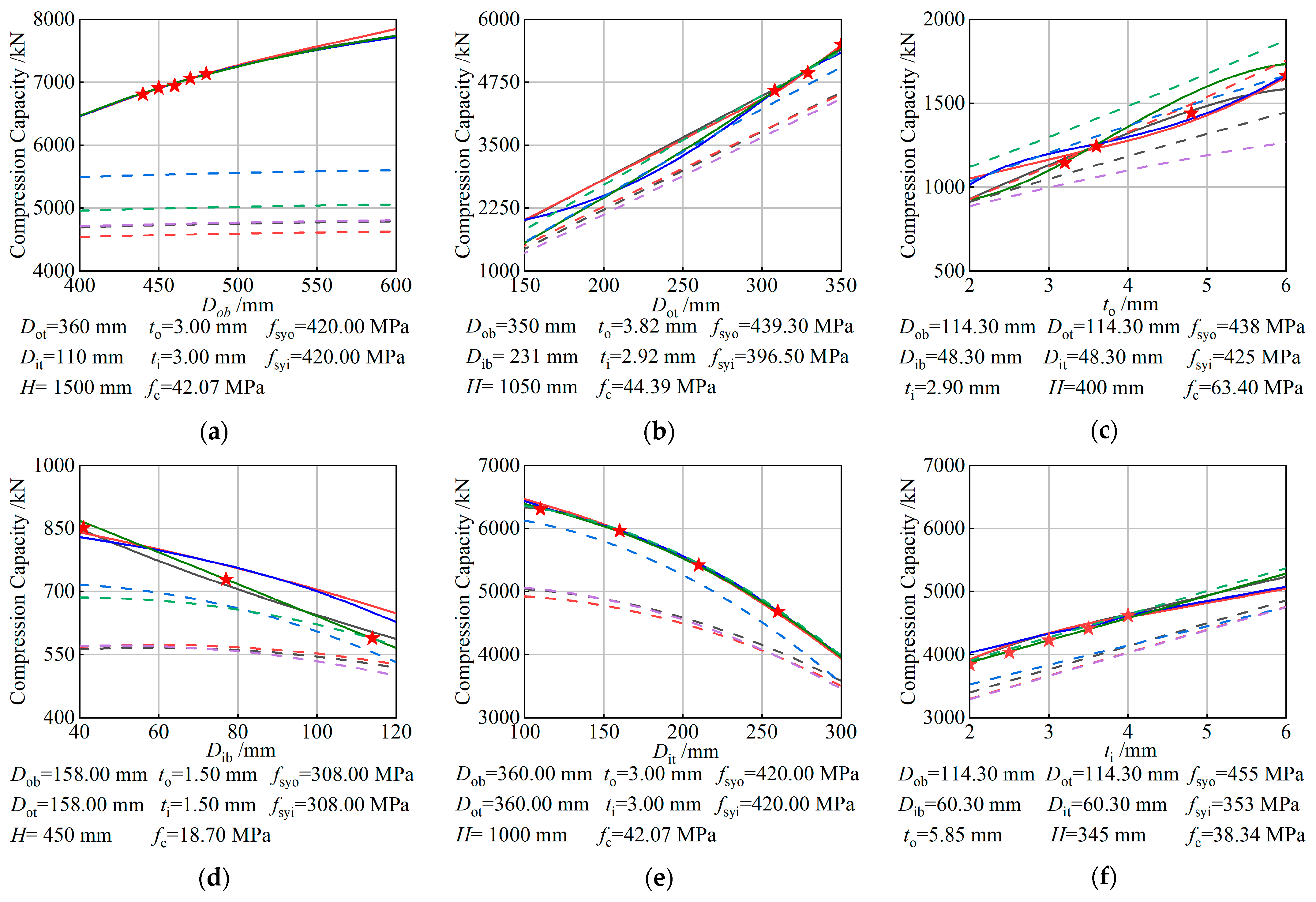
6. Parametric Analysis of Predictive Models
7. Conclusions
- (1)
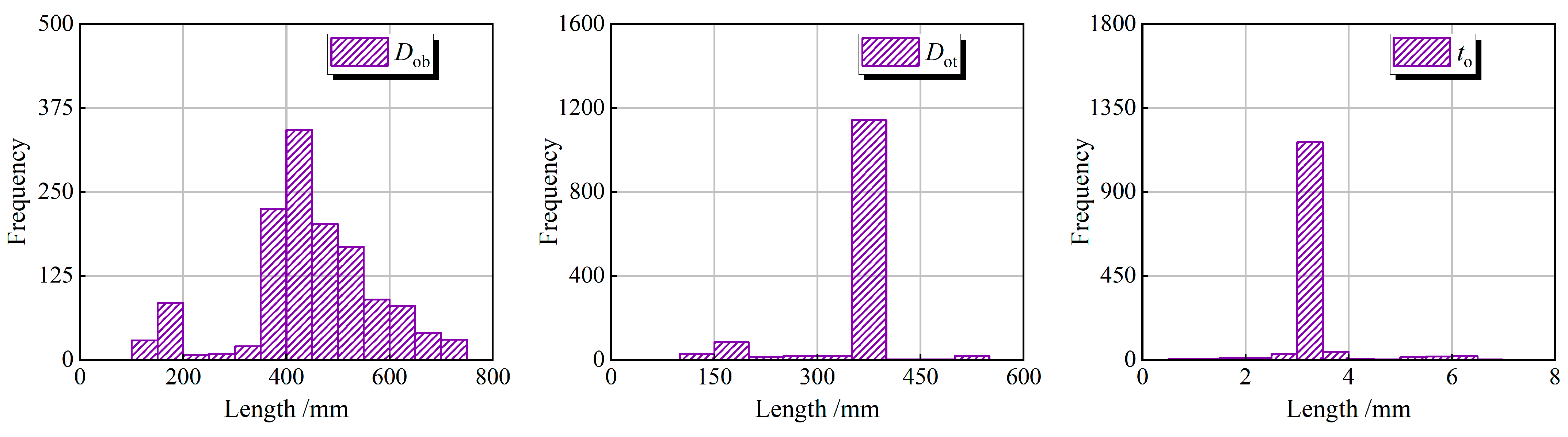
- The database established in this study uses the basic dimensions of the components (outer steel tube bottom diameter, outer steel tube top diameter, outer steel tube wall thickness, inner steel tube bottom diameter, inner steel tube top diameter, inner steel tube wall thickness, and component length) and material strengths (concrete strength, outer steel tube yield strength, and inner steel tube yield strength) as input parameters, with the axial load-bearing capacity of TCFDST components as the output variable. The sample distribution of the database exhibits a bell-shaped curve, approximately following a normal distribution, which indicates good characteristics for data analysis.
- (2)
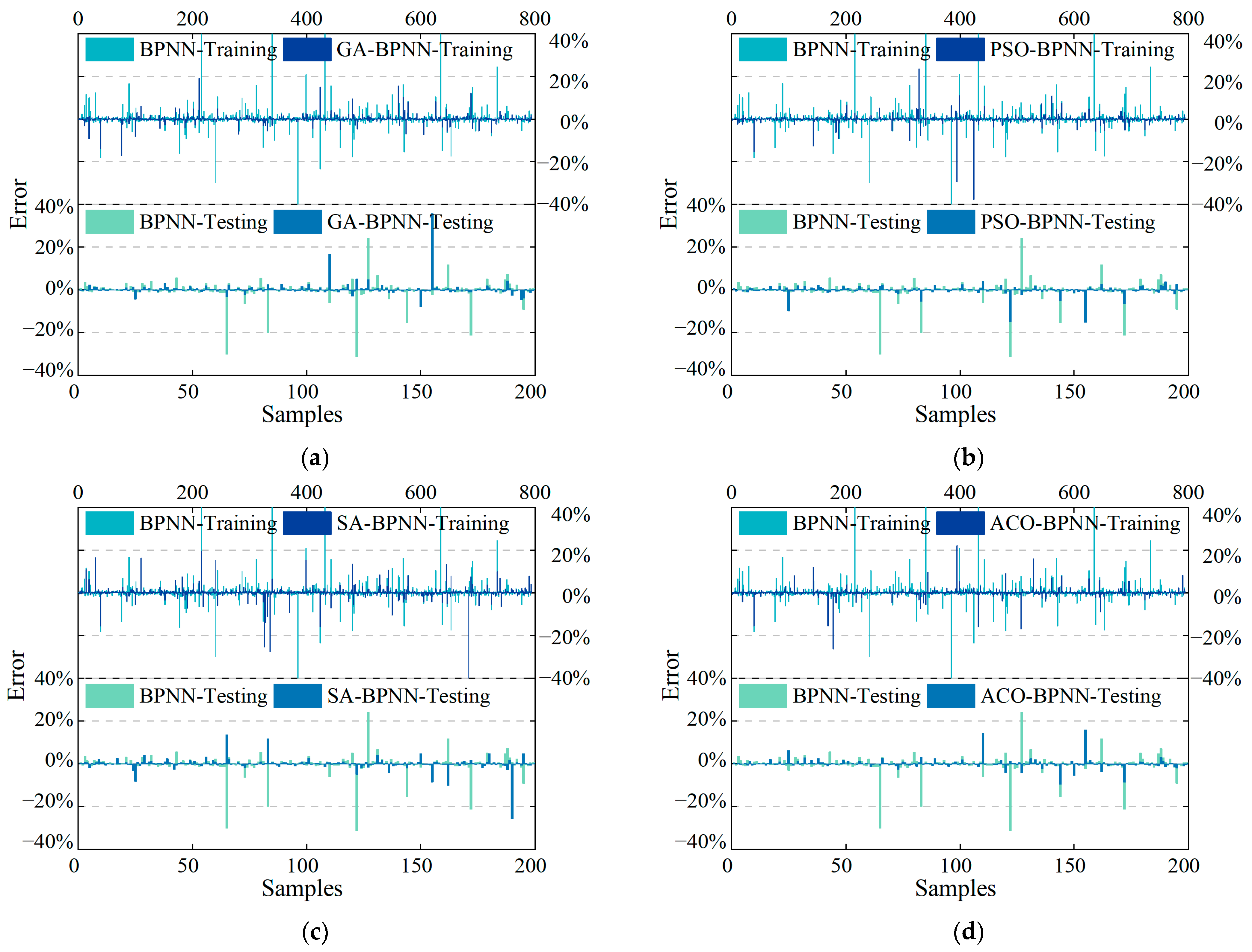
- The heuristic-algorithm-optimized BPNN predictive models for axial load-bearing capacity demonstrate smaller prediction errors across the training, validation, and test sets compared to the standard BPNN, RF, KNN, SVR, and RBFNN models. The goodness of fit for the test set improved after model optimization.
- (3)
- The heuristic-algorithm-optimized BPNN predictive models show better accuracy in predicting axial load-bearing capacity on both the test and training sets compared to the national standard formulas, with the goodness of fit (R2) exceeding 0.99 and the mean absolute percentage error (MAPE) being less than 2%.
- (4)
- The parametric analysis indicates that the heuristic-algorithm-optimized BPNN predictive models can effectively capture the relationship between input variables and axial load-bearing capacity, showing consistency with the results obtained from standard formulas and providing higher accuracy.
- (5)
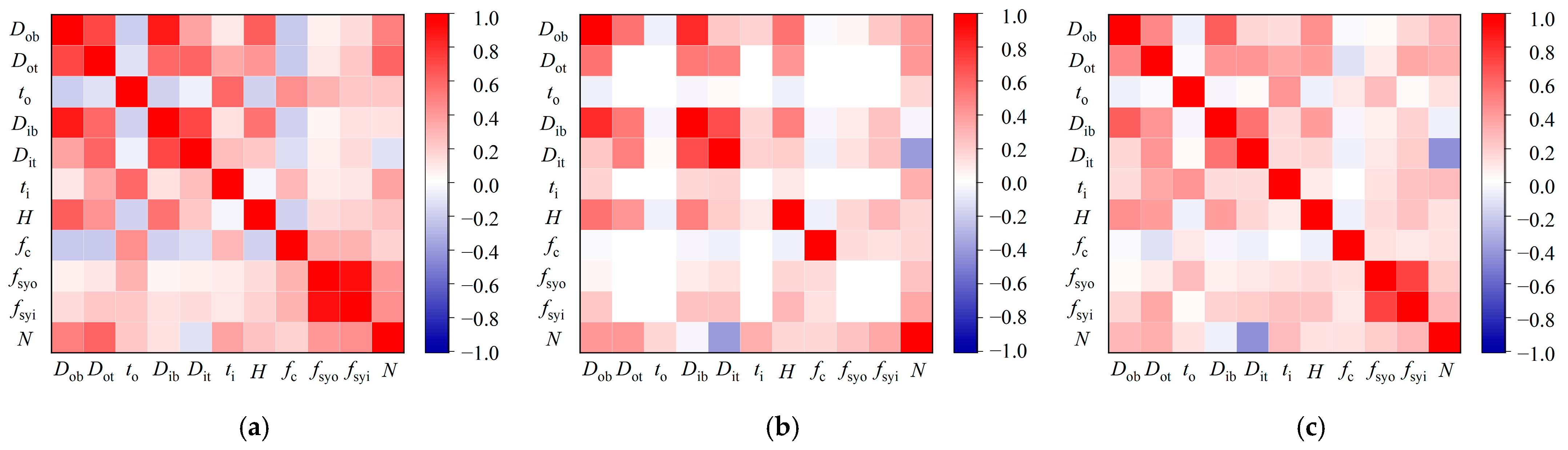
- To enhance the interpretability of the predictive models, LIME was applied, providing a deeper understanding of the contribution of each input parameter to the model’s predictions. The analysis revealed that key features such as outer steel tube diameter (top and bottom), outer tube thickness, inner steel tube diameter (top and bottom), inner tube thickness, height, sandwich concrete strength, yield strength of the outer tube, and yield strength of the inner tube play significant roles in determining the axial load-bearing capacity. The combination of high accuracy and improved interpretability makes these models highly valuable for practical engineering applications, allowing for more transparent and data-driven decision-making in the design and optimization of TCFDST components.
Author Contributions
Funding
Data Availability Statement
Acknowledgments
Conflicts of Interest
Abbreviations
| TCFDST | tapered concrete-filled double-skin steel tubular |
| CFDST | concrete-filled double-skin steel tubular |
| CFST | concrete-filled steel tubular |
| GA | Genetic Algorithm |
| PSO | Particle Swarm Optimization |
| SA | Simulated Annealing |
| ACO | Ant Colony Optimization |
| SCSO | symbiotic organism search optimization |
| GWO_WOA | grey wolf optimizer and whale optimization algorithm |
| ARO | artificial rabbit optimization |
| GBR | gradient boosting regression |
| SVM | support vector machine |
| RFR | random forest regression |
| NN | neural network |
| KNN | K-Nearest Neighbors |
| tensile strain of steel | |
| tensile stress of steel | |
| elastic model of steel | |
| yield strength of steel | |
| tensile strength of steel | |
| compression strength of concrete cylinder | |
| outer diameter of the outer steel tube at the bottom of the specimen | |
| outer diameter of the outer steel tube at the top of the specimen | |
| thickness of the outer steel tube | |
| yield strength of the outer steel tube | |
| outer diameter of the inner steel tube at the bottom of the specimen | |
| outer diameter of the inner steel tube at the top of the specimen | |
| thickness of the inner steel tube | |
| yield strength of the inner steel tube | |
| height of the specimen | |
| compression bearing capacity | |
| compressive strength of a concrete cylinder with a diameter of 100 mm | |
| compressive strength of a concrete cylinder with a diameter of 150 mm | |
| compressive strength of a concrete cube with a diameter of 100 mm | |
| compressive strength of a concrete cube with a diameter of 150 mm | |
| input parameters of BPNN input layer node i | |
| the weight of input node i corresponding to hidden layer node h | |
| input parameters of BPNN hidden layer node h | |
| output parameters of BPNN hidden layer node h | |
| the weight of hidden layer node h corresponding to output layer node j | |
| input parameters of BPNN output layer node j | |
| output parameters of BPNN output layer node j | |
| area of the outer steel tube | |
| area of the inner steel tube | |
| section moment of inertia of the outer steel tube | |
| section moment of inertia of the sandwich concrete |
Appendix A. Detailed Information of Test 192 Column Under Compression
| Specimen Label | Outer Tube Dimensions (mm) | Inner Tube Dimensions (mm) | /mm | /° | Materials (MPa) | /kN | |||||||
| CFDST-ZY-1A | 360.00 | 338.00 | 3.12 | 300.00 | 278.00 | 3.12 | 1080.00 | 0.58 | 0.84 | 788.00 | 788.00 | 117.74 | 6800.00 |
| CFDST-ZY-2A | 300.00 | 282.00 | 3.12 | 240.00 | 222.00 | 3.12 | 900.00 | 0.57 | 0.81 | 788.00 | 788.00 | 117.74 | 6051.00 |
| CFDST-ZY-3A | 300.00 | 282.00 | 3.12 | 240.00 | 222.00 | 3.97 | 900.00 | 0.57 | 0.81 | 788.00 | 755.00 | 117.74 | 6616.00 |
| CFDST-ZY-4A | 300.00 | 282.00 | 3.97 | 210.00 | 192.00 | 5.97 | 900.00 | 0.57 | 0.70 | 755.00 | 708.00 | 117.74 | 9577.00 |
| CFDST-ZY-5A | 300.00 | 282.00 | 5.97 | 210.00 | 192.00 | 5.97 | 900.00 | 0.57 | 0.71 | 708.00 | 708.00 | 117.74 | 9950.00 |
| C1-1/2 | 350.00 | 350.00 | 3.82 | 231.00 | 231.00 | 2.92 | 1050.00 | 0.00 | 0.67 | 439.30 | 396.50 | 44.39 | 5448.00 |
| C2-1/2 | 350.00 | 329.00 | 3.82 | 231.00 | 210.00 | 2.92 | 1050.00 | 0.57 | 0.65 | 439.30 | 396.50 | 44.39 | 4932.00 |
| C3-1/2 | 350.00 | 308.00 | 3.82 | 231.00 | 189.00 | 2.92 | 1050.00 | 1.15 | 0.63 | 439.30 | 396.50 | 44.39 | 4585.00 |
| C4-1/2 | 300.00 | 282.00 | 3.82 | 198.00 | 180.00 | 2.92 | 900.00 | 0.57 | 0.66 | 439.30 | 396.50 | 44.39 | 3961.00 |
| C5-1/2 | 250.00 | 235.00 | 3.82 | 165.00 | 150.00 | 2.92 | 750.00 | 0.57 | 0.66 | 439.30 | 396.50 | 44.39 | 3103.00 |
| CT1-1 | 170.00 | 160.00 | 2.78 | 115.00 | 105.00 | 2.78 | 510.00 | 0.56 | 0.68 | 281.00 | 281.00 | 52.94 | 1228.00 |
| CT1-2 | 170.00 | 160.00 | 2.78 | 115.00 | 105.00 | 2.78 | 510.00 | 0.56 | 0.68 | 281.00 | 281.00 | 52.94 | 1229.00 |
| CT2-1 | 170.00 | 160.00 | 2.78 | 131.00 | 121.00 | 2.78 | 510.00 | 0.56 | 0.78 | 281.00 | 281.00 | 52.94 | 1108.00 |
| CT2-2 | 170.00 | 160.00 | 2.78 | 131.00 | 121.00 | 2.78 | 510.00 | 0.56 | 0.78 | 281.00 | 281.00 | 52.94 | 1100.00 |
| CT3-1 | 180.00 | 169.00 | 2.78 | 122.00 | 111.00 | 2.78 | 540.00 | 0.58 | 0.68 | 281.00 | 281.00 | 52.94 | 1320.00 |
| CT3-2 | 180.00 | 169.00 | 2.78 | 122.00 | 111.00 | 2.78 | 540.00 | 0.58 | 0.68 | 281.00 | 281.00 | 52.94 | 1380.00 |
| CT4-1 | 180.00 | 169.00 | 2.78 | 139.00 | 128.00 | 2.78 | 540.00 | 0.58 | 0.78 | 281.00 | 281.00 | 52.94 | 1152.00 |
| CT4-2 | 180.00 | 169.00 | 2.78 | 139.00 | 128.00 | 2.78 | 540.00 | 0.58 | 0.78 | 281.00 | 281.00 | 52.94 | 1170.00 |
| CT5-1 | 190.00 | 179.00 | 2.78 | 129.00 | 118.00 | 2.78 | 570.00 | 0.55 | 0.68 | 281.00 | 281.00 | 52.94 | 1420.00 |
| CT5-2 | 190.00 | 179.00 | 2.78 | 129.00 | 118.00 | 2.78 | 570.00 | 0.55 | 0.68 | 281.00 | 281.00 | 52.94 | 1360.00 |
| CT6-1 | 190.00 | 179.00 | 2.78 | 147.00 | 136.00 | 2.78 | 570.00 | 0.55 | 0.78 | 281.00 | 281.00 | 52.94 | 1240.00 |
| CT6-2 | 190.00 | 179.00 | 2.78 | 147.00 | 136.00 | 2.78 | 570.00 | 0.55 | 0.78 | 281.00 | 281.00 | 52.94 | 1270.00 |
| cc2a | 180.00 | 180.00 | 3.00 | 48.00 | 48.00 | 3.00 | 540.00 | 0.00 | 0.28 | 275.90 | 396.10 | 39.66 | 1790.00 |
| cc3a | 180.00 | 180.00 | 3.00 | 88.00 | 88.00 | 3.00 | 540.00 | 0.00 | 0.51 | 275.90 | 370.20 | 39.66 | 1648.00 |
| cc4a | 180.00 | 180.00 | 3.00 | 140.00 | 140.00 | 3.00 | 540.00 | 0.00 | 0.80 | 275.90 | 342.00 | 39.66 | 1435.00 |
| cc5a | 114.00 | 114.00 | 3.00 | 58.00 | 58.00 | 3.00 | 342.00 | 0.00 | 0.54 | 294.50 | 374.50 | 39.66 | 904.00 |
| cc6a | 240.00 | 240.00 | 3.00 | 114.00 | 114.00 | 3.00 | 720.00 | 0.00 | 0.49 | 275.90 | 294.50 | 39.66 | 2421.00 |
| cc7a | 300.00 | 300.00 | 3.00 | 165.00 | 165.00 | 3.00 | 900.00 | 0.00 | 0.56 | 275.90 | 320.50 | 39.66 | 3331.00 |
| CC-DS-N | 165.00 | 165.00 | 3.54 | 60.00 | 60.00 | 2.85 | 480.00 | 0.00 | 0.38 | 368.00 | 394.00 | 42.53 | 1660.00 |
| Aa-0.8 | 538.00 | 538.00 | 3.76 | 418.00 | 418.00 | 5.63 | 1500.00 | 0.00 | 0.79 | 253.80 | 296.30 | 57.69 | 8949.70 |
| Aa-0.85 | 538.00 | 538.00 | 3.76 | 449.00 | 449.00 | 5.63 | 1500.00 | 0.00 | 0.85 | 253.80 | 296.30 | 57.69 | 7924.70 |
| Aa-0.9 | 538.00 | 538.00 | 3.76 | 477.00 | 477.00 | 5.63 | 1500.00 | 0.00 | 0.90 | 253.80 | 296.30 | 57.69 | 6036.70 |
| Ab-0.8 | 538.00 | 538.00 | 3.76 | 418.00 | 418.00 | 5.63 | 1500.00 | 0.00 | 0.79 | 253.80 | 296.30 | 41.51 | 7896.60 |
| Ab-0.85 | 538.00 | 538.00 | 3.76 | 449.00 | 449.00 | 5.63 | 1500.00 | 0.00 | 0.85 | 253.80 | 296.30 | 41.51 | 6735.20 |
| Ab-0.9 | 538.00 | 538.00 | 3.76 | 477.00 | 477.00 | 5.63 | 1500.00 | 0.00 | 0.90 | 253.80 | 296.30 | 41.51 | 5966.80 |
| Bb-0.8 | 538.00 | 538.00 | 5.63 | 420.00 | 420.00 | 5.63 | 1500.00 | 0.00 | 0.80 | 296.30 | 296.30 | 41.51 | 8864.00 |
| Bb-0.85 | 538.00 | 538.00 | 5.63 | 448.00 | 448.00 | 5.63 | 1500.00 | 0.00 | 0.85 | 296.30 | 296.30 | 41.51 | 8068.00 |
| Bb-0.9 | 538.00 | 538.00 | 5.63 | 473.00 | 473.00 | 5.63 | 1500.00 | 0.00 | 0.90 | 296.30 | 296.30 | 41.51 | 6774.00 |
| C4-46-0.26-3.7-1 | 165.20 | 165.20 | 3.68 | 42.50 | 42.50 | 3.19 | 495.00 | 0.00 | 0.27 | 357.70 | 409.80 | 53.70 | 2060.00 |
| C4-83-0.26-3.7-1 | 165.00 | 165.00 | 3.68 | 42.60 | 42.60 | 3.21 | 495.00 | 0.00 | 0.27 | 357.70 | 409.80 | 90.70 | 2423.00 |
| C4-130-0.26-3.7-1 | 164.80 | 164.80 | 3.69 | 42.60 | 42.60 | 3.20 | 495.00 | 0.00 | 0.27 | 357.70 | 409.80 | 141.00 | 3068.00 |
| C4-46-0.46-3.7-1 | 165.00 | 165.00 | 3.70 | 76.00 | 76.00 | 2.80 | 495.00 | 0.00 | 0.48 | 357.70 | 385.60 | 53.70 | 1831.00 |
| C4-83-0.46-3.7-1 | 165.10 | 165.10 | 3.67 | 76.10 | 76.10 | 2.81 | 495.00 | 0.00 | 0.48 | 357.70 | 385.60 | 90.70 | 2174.00 |
| C4-130-0.46-3.7-1 | 164.80 | 164.80 | 3.68 | 76.30 | 76.30 | 2.80 | 495.00 | 0.00 | 0.48 | 357.70 | 385.60 | 141.00 | 2732.00 |
| C4-46-0.46-6.0-1 | 165.30 | 165.30 | 5.96 | 76.10 | 76.10 | 2.79 | 495.00 | 0.00 | 0.50 | 347.00 | 385.60 | 53.70 | 2183.00 |
| C4-83-0.46-6.0-1 | 164.90 | 164.90 | 6.01 | 75.90 | 75.90 | 2.80 | 495.00 | 0.00 | 0.50 | 347.00 | 385.60 | 90.70 | 2666.00 |
| C4-130-0.46-6.0-1 | 164.90 | 164.90 | 6.01 | 76.00 | 76.00 | 2.81 | 495.00 | 0.00 | 0.50 | 347.00 | 385.60 | 141.00 | 3110.00 |
| C9-46-0.46-6.0-1 | 165.20 | 165.20 | 5.95 | 76.10 | 76.10 | 2.79 | 495.00 | 0.00 | 0.50 | 428.60 | 385.60 | 53.70 | 2645.00 |
| C9-83-0.46-6.0-1 | 165.00 | 165.00 | 5.99 | 75.80 | 75.80 | 2.80 | 495.00 | 0.00 | 0.50 | 428.60 | 385.60 | 90.70 | 2971.00 |
| C9-130-0.46-6.0-1 | 165.10 | 165.10 | 5.94 | 75.90 | 75.90 | 2.80 | 495.00 | 0.00 | 0.50 | 428.60 | 385.60 | 141.00 | 3322.00 |
| C10-375 | 158.00 | 158.00 | 0.90 | 38.00 | 38.00 | 0.90 | 450.00 | 0.00 | 0.24 | 221.00 | 221.00 | 18.70 | 635.00 |
| C10-750 | 159.00 | 159.00 | 0.90 | 76.00 | 76.00 | 0.90 | 450.00 | 0.00 | 0.48 | 221.00 | 221.00 | 18.70 | 540.00 |
| C10-1125 | 159.00 | 159.00 | 0.90 | 114.00 | 114.00 | 0.90 | 450.00 | 0.00 | 0.73 | 221.00 | 221.00 | 18.70 | 378.00 |
| C16-375 | 158.00 | 158.00 | 1.50 | 39.00 | 39.00 | 1.50 | 450.00 | 0.00 | 0.25 | 308.00 | 308.00 | 18.70 | 851.60 |
| C16-750 | 158.00 | 158.00 | 1.50 | 77.00 | 77.00 | 1.50 | 450.00 | 0.00 | 0.50 | 308.00 | 308.00 | 18.70 | 728.10 |
| C16-1125 | 158.00 | 158.00 | 1.50 | 114.00 | 114.00 | 1.50 | 450.00 | 0.00 | 0.74 | 308.00 | 308.00 | 18.70 | 589.00 |
| C23-375 | 158.00 | 158.00 | 2.14 | 40.00 | 40.00 | 2.14 | 450.00 | 0.00 | 0.26 | 286.00 | 286.00 | 18.70 | 968.20 |
| C23-750 | 158.00 | 158.00 | 2.14 | 77.00 | 77.00 | 2.14 | 450.00 | 0.00 | 0.50 | 286.00 | 286.00 | 18.70 | 879.10 |
| C23-1125 | 157.00 | 157.00 | 2.14 | 115.00 | 115.00 | 2.14 | 450.00 | 0.00 | 0.75 | 286.00 | 286.00 | 18.70 | 703.60 |
| C1-1 | 356.00 | 356.00 | 5.50 | 219.00 | 219.00 | 3.30 | 1068.00 | 0.00 | 0.63 | 618.00 | 356.00 | 38.83 | 7242.00 |
| C2-2 | 356.00 | 356.00 | 5.50 | 168.00 | 168.00 | 3.30 | 1068.00 | 0.00 | 0.49 | 618.00 | 356.00 | 38.83 | 8516.00 |
| 1-1-2 | 114.30 | 114.30 | 5.85 | 60.30 | 60.30 | 2.52 | 345.00 | 0.00 | 0.59 | 455.00 | 396.00 | 38.34 | 1421.54 |
| 2-1-2 | 114.30 | 114.30 | 5.85 | 60.30 | 60.30 | 5.77 | 345.00 | 0.00 | 0.59 | 455.00 | 310.00 | 38.34 | 1574.26 |
| 1-1-1 | 114.30 | 114.30 | 2.73 | 60.30 | 60.30 | 2.52 | 345.00 | 0.00 | 0.55 | 285.00 | 396.00 | 38.34 | 734.60 |
| 2-1-1 | 114.30 | 114.30 | 2.73 | 60.30 | 60.30 | 5.77 | 345.00 | 0.00 | 0.55 | 285.00 | 310.00 | 38.34 | 913.07 |
| 1-2-2 | 114.30 | 114.30 | 5.85 | 60.30 | 60.30 | 2.52 | 345.00 | 0.00 | 0.59 | 455.00 | 396.00 | 64.14 | 1505.67 |
| 2-2-2 | 114.30 | 114.30 | 5.85 | 60.30 | 60.30 | 5.77 | 345.00 | 0.00 | 0.59 | 455.00 | 310.00 | 64.14 | 1666.41 |
| 1-2-1 | 114.30 | 114.30 | 2.73 | 60.30 | 60.30 | 2.52 | 345.00 | 0.00 | 0.55 | 285.00 | 396.00 | 64.14 | 899.21 |
| 2-2-1 | 114.30 | 114.30 | 2.73 | 60.30 | 60.30 | 5.77 | 345.00 | 0.00 | 0.55 | 285.00 | 310.00 | 64.14 | 1088.06 |
| C4-36-0.18-5-1 | 190.60 | 190.60 | 5.15 | 34.00 | 34.00 | 3.08 | 570.00 | 0.00 | 0.19 | 346.90 | 348.20 | 37.50 | 2718.00 |
| C4-36-0.31-5-1 | 190.50 | 190.50 | 5.15 | 59.60 | 59.60 | 3.32 | 570.00 | 0.00 | 0.33 | 346.90 | 342.10 | 37.50 | 2718.00 |
| C4-36-0.53-5-1 | 190.70 | 190.70 | 5.11 | 101.60 | 101.60 | 4.03 | 570.00 | 0.00 | 0.56 | 346.90 | 345.80 | 37.50 | 2626.00 |
| C9-36-0.18-5-1 | 188.90 | 188.90 | 5.09 | 33.70 | 33.70 | 3.09 | 570.00 | 0.00 | 0.19 | 464.00 | 348.20 | 37.50 | 3182.00 |
| C9-36-0.31-5-1 | 191.00 | 191.00 | 5.15 | 59.40 | 59.40 | 3.31 | 570.00 | 0.00 | 0.33 | 464.00 | 342.10 | 37.50 | 3286.00 |
| C9-36-0.53-5-1 | 190.70 | 190.70 | 5.15 | 101.10 | 101.10 | 4.10 | 570.00 | 0.00 | 0.56 | 464.00 | 345.80 | 37.50 | 3082.00 |
| C4-24-0.31-5-1 | 190.40 | 190.40 | 5.15 | 59.90 | 59.90 | 3.33 | 570.00 | 0.00 | 0.33 | 346.90 | 342.10 | 29.00 | 2460.00 |
| C4-36-0.31-5-1 | 189.10 | 189.10 | 5.10 | 59.40 | 59.40 | 3.35 | 570.00 | 0.00 | 0.33 | 346.90 | 342.10 | 37.50 | 2623.00 |
| C4-48-0.31-5-1 | 189.90 | 189.90 | 5.12 | 58.90 | 58.90 | 3.31 | 570.00 | 0.00 | 0.33 | 346.90 | 342.10 | 51.00 | 2950.00 |
| C4-36-0.31-4-1 | 190.30 | 190.30 | 4.26 | 59.40 | 59.40 | 3.36 | 570.00 | 0.00 | 0.33 | 336.80 | 342.10 | 37.50 | 2376.00 |
| C4-36-0.31-5-1 | 189.70 | 189.70 | 5.12 | 59.50 | 59.50 | 3.32 | 570.00 | 0.00 | 0.33 | 346.90 | 342.10 | 37.50 | 2611.00 |
| C4-36-0.31-6-1 | 189.10 | 189.10 | 6.77 | 59.70 | 59.70 | 3.34 | 570.00 | 0.00 | 0.34 | 327.30 | 342.10 | 37.50 | 2894.00 |
| C-1 | 398.00 | 340.00 | 3.00 | 332.00 | 274.00 | 2.50 | 1465.00 | 1.13 | 0.82 | 326.67 | 336.67 | 30.74 | 2391.00 |
| C-2 | 398.00 | 300.00 | 3.00 | 332.00 | 234.00 | 2.50 | 1465.00 | 1.92 | 0.80 | 326.67 | 336.67 | 30.74 | 2350.00 |
| C-4 | 398.00 | 340.00 | 3.00 | 312.00 | 254.00 | 2.50 | 1465.00 | 1.13 | 0.76 | 326.67 | 336.67 | 30.74 | 2599.00 |
| C-5 | 398.00 | 340.00 | 3.00 | 292.00 | 234.00 | 2.50 | 1465.00 | 1.13 | 0.70 | 326.67 | 336.67 | 30.74 | 2885.00 |
| C-6 | 398.00 | 340.00 | 3.50 | 332.00 | 274.00 | 3.00 | 1465.00 | 1.13 | 0.82 | 350.00 | 326.67 | 30.74 | 2555.00 |
| C-7 | 398.00 | 340.00 | 2.50 | 332.00 | 274.00 | 2.00 | 1465.00 | 1.13 | 0.82 | 336.67 | 305.00 | 30.74 | 2094.00 |
| S139.2-1.0 | 139.20 | 139.20 | 3.00 | 76.00 | 76.00 | 2.00 | 1000.00 | 0.00 | 0.57 | 418.00 | 324.00 | 27.72 | 1059.20 |
| S139.2-1.5 | 139.20 | 139.20 | 3.00 | 76.00 | 76.00 | 2.00 | 1500.00 | 0.00 | 0.57 | 418.00 | 324.00 | 27.72 | 905.50 |
| S139.2-2.0 | 139.20 | 139.20 | 3.00 | 76.00 | 76.00 | 2.00 | 2000.00 | 0.00 | 0.57 | 418.00 | 324.00 | 27.72 | 831.70 |
| S139.2-2.5 | 139.20 | 139.20 | 3.00 | 76.00 | 76.00 | 2.00 | 2500.00 | 0.00 | 0.57 | 418.00 | 324.00 | 27.72 | 732.10 |
| S152.4-1.0 | 152.40 | 152.40 | 3.00 | 76.00 | 76.00 | 2.00 | 1000.00 | 0.00 | 0.52 | 549.00 | 324.00 | 27.72 | 1263.50 |
| S152.4-1.5 | 152.40 | 152.40 | 3.00 | 76.00 | 76.00 | 2.00 | 1500.00 | 0.00 | 0.52 | 549.00 | 324.00 | 27.72 | 1195.60 |
| S152.4-2.0 | 152.40 | 152.40 | 3.00 | 76.00 | 76.00 | 2.00 | 2000.00 | 0.00 | 0.52 | 549.00 | 324.00 | 27.72 | 1047.30 |
| S152.4-2.5 | 152.40 | 152.40 | 3.00 | 76.00 | 76.00 | 2.00 | 2500.00 | 0.00 | 0.52 | 549.00 | 324.00 | 27.72 | 941.40 |
| S165.1-1.0 | 165.00 | 165.00 | 3.00 | 76.00 | 76.00 | 2.00 | 1000.00 | 0.00 | 0.48 | 516.00 | 324.00 | 27.72 | 1512.30 |
| S165.1-1.5 | 165.00 | 165.00 | 3.00 | 76.00 | 76.00 | 2.00 | 1500.00 | 0.00 | 0.48 | 516.00 | 324.00 | 27.72 | 1286.40 |
| S165.1-2.0 | 165.00 | 165.00 | 3.00 | 76.00 | 76.00 | 2.00 | 2000.00 | 0.00 | 0.48 | 516.00 | 324.00 | 27.72 | 1187.20 |
| S165.1-2.5 | 165.00 | 165.00 | 3.00 | 76.00 | 76.00 | 2.00 | 2500.00 | 0.00 | 0.48 | 516.00 | 324.00 | 27.72 | 1028.00 |
| S193.7-1.0 | 193.70 | 193.70 | 3.50 | 76.00 | 76.00 | 2.00 | 1000.00 | 0.00 | 0.41 | 391.00 | 324.00 | 27.72 | 2010.00 |
| S193.7-1.5 | 193.70 | 193.70 | 3.50 | 76.00 | 76.00 | 2.00 | 1500.00 | 0.00 | 0.41 | 391.00 | 324.00 | 27.72 | 1730.00 |
| S193.7-2.0 | 193.70 | 193.70 | 3.50 | 76.00 | 76.00 | 2.00 | 2000.00 | 0.00 | 0.41 | 391.00 | 324.00 | 27.72 | 1581.60 |
| S193.7-2.5 | 193.70 | 193.70 | 3.50 | 76.00 | 76.00 | 2.00 | 2500.00 | 0.00 | 0.41 | 391.00 | 324.00 | 27.72 | 1451.40 |
| CFT-A1 | 140.00 | 140.00 | 3.00 | 48.00 | 48.00 | 5.00 | 500.00 | 0.00 | 0.36 | 285.00 | 290.00 | 37.82 | 1232.40 |
| CFT-A2 | 140.00 | 140.00 | 3.00 | 58.00 | 58.00 | 5.00 | 500.00 | 0.00 | 0.43 | 285.00 | 290.00 | 37.82 | 1223.70 |
| CFT-A3 | 140.00 | 140.00 | 5.00 | 68.00 | 68.00 | 3.00 | 500.00 | 0.00 | 0.52 | 290.00 | 285.00 | 37.82 | 1347.00 |
| CFT-A4 | 140.00 | 140.00 | 5.00 | 78.00 | 78.00 | 3.00 | 500.00 | 0.00 | 0.60 | 290.00 | 285.00 | 37.82 | 1334.30 |
| CFT-B1 | 180.00 | 180.00 | 3.00 | 48.00 | 48.00 | 5.00 | 500.00 | 0.00 | 0.28 | 300.00 | 320.00 | 37.82 | 1852.20 |
| CFT-B2 | 180.00 | 180.00 | 3.00 | 58.00 | 58.00 | 5.00 | 500.00 | 0.00 | 0.33 | 300.00 | 320.00 | 37.82 | 1841.40 |
| CFT-B3 | 180.00 | 180.00 | 5.00 | 68.00 | 68.00 | 3.00 | 500.00 | 0.00 | 0.40 | 320.00 | 300.00 | 37.82 | 2057.50 |
| CFT-B4 | 180.00 | 180.00 | 5.00 | 78.00 | 78.00 | 3.00 | 500.00 | 0.00 | 0.46 | 320.00 | 300.00 | 37.82 | 2043.30 |
| O1I1 | 114.30 | 114.30 | 6.00 | 48.30 | 48.30 | 2.90 | 400.00 | 0.00 | 0.47 | 454.00 | 425.00 | 63.40 | 1665.00 |
| O2I1 | 114.30 | 114.30 | 4.80 | 48.30 | 48.30 | 2.90 | 400.00 | 0.00 | 0.46 | 416.00 | 425.00 | 63.40 | 1441.00 |
| O3I1 | 114.30 | 114.30 | 3.60 | 48.30 | 48.30 | 2.90 | 400.00 | 0.00 | 0.45 | 453.00 | 425.00 | 63.40 | 1243.00 |
| O4I1 | 114.30 | 114.30 | 3.20 | 48.30 | 48.30 | 2.90 | 400.00 | 0.00 | 0.45 | 430.00 | 425.00 | 63.40 | 1145.00 |
| O5I2 | 165.10 | 165.10 | 3.50 | 101.60 | 101.60 | 3.30 | 500.00 | 0.00 | 0.64 | 433.00 | 394.00 | 63.40 | 1629.00 |
| O6I2 | 165.10 | 165.10 | 3.00 | 101.60 | 101.60 | 3.20 | 500.00 | 0.00 | 0.64 | 395.00 | 394.00 | 63.40 | 1613.00 |
| O7I2 | 163.80 | 163.80 | 2.35 | 101.60 | 101.60 | 3.20 | 500.00 | 0.00 | 0.64 | 395.00 | 394.00 | 63.40 | 1487.00 |
| O8I2 | 163.00 | 163.00 | 1.95 | 101.60 | 101.60 | 3.20 | 500.00 | 0.00 | 0.64 | 395.00 | 394.00 | 63.40 | 1328.00 |
| O9I2 | 162.50 | 162.50 | 1.70 | 101.60 | 101.60 | 3.20 | 500.00 | 0.00 | 0.64 | 395.00 | 394.00 | 63.40 | 1236.00 |
| CA-0.8-a | 538.00 | 538.00 | 3.76 | 418.00 | 418.00 | 5.63 | 1507.00 | 0.00 | 0.79 | 253.80 | 296.30 | 57.69 | 8949.70 |
| CA-0.85-a | 538.00 | 538.00 | 3.76 | 449.00 | 449.00 | 5.63 | 1507.00 | 0.00 | 0.85 | 253.80 | 296.30 | 57.69 | 7924.70 |
| CA-0.9-a | 538.00 | 538.00 | 3.76 | 477.00 | 477.00 | 5.63 | 1507.00 | 0.00 | 0.90 | 253.80 | 296.30 | 57.69 | 6036.70 |
| CA-0.8-b | 538.00 | 538.00 | 3.76 | 418.00 | 418.00 | 5.63 | 1507.00 | 0.00 | 0.79 | 253.80 | 296.30 | 41.51 | 7896.60 |
| CA-0.85-b | 538.00 | 538.00 | 3.76 | 449.00 | 449.00 | 5.63 | 1507.00 | 0.00 | 0.85 | 253.80 | 296.30 | 41.51 | 6735.20 |
| CA-0.9-b | 538.00 | 538.00 | 3.76 | 477.00 | 477.00 | 5.63 | 1507.00 | 0.00 | 0.90 | 253.80 | 296.30 | 41.51 | 5966.80 |
| CB-0.8-b | 538.00 | 538.00 | 5.63 | 420.00 | 420.00 | 5.63 | 1507.00 | 0.00 | 0.80 | 296.30 | 296.30 | 41.51 | 8864.00 |
| CB-0.85-b | 538.00 | 538.00 | 5.63 | 448.00 | 448.00 | 5.63 | 1507.00 | 0.00 | 0.85 | 296.30 | 296.30 | 41.51 | 8068.00 |
| CB-0.9-b | 538.00 | 538.00 | 5.63 | 473.00 | 473.00 | 5.63 | 1507.00 | 0.00 | 0.90 | 296.30 | 296.30 | 41.51 | 6774.00 |
| 1 | 160.00 | 160.00 | 1.00 | 37.00 | 37.00 | 1.00 | 400.00 | 0.00 | 0.23 | 220.00 | 220.00 | 23.60 | 635.00 |
| 2 | 160.00 | 160.00 | 1.00 | 75.00 | 75.00 | 1.00 | 400.00 | 0.00 | 0.47 | 220.00 | 220.00 | 23.60 | 540.00 |
| 3 | 160.00 | 160.00 | 1.00 | 112.00 | 112.00 | 1.00 | 400.00 | 0.00 | 0.71 | 220.00 | 220.00 | 23.60 | 378.00 |
| 4 | 160.00 | 160.00 | 1.50 | 37.00 | 37.00 | 1.50 | 400.00 | 0.00 | 0.24 | 255.00 | 255.00 | 23.60 | 851.00 |
| 5 | 160.00 | 160.00 | 1.50 | 75.00 | 75.00 | 1.50 | 400.00 | 0.00 | 0.48 | 255.00 | 255.00 | 23.60 | 728.00 |
| 6 | 160.00 | 160.00 | 1.50 | 112.00 | 112.00 | 1.50 | 400.00 | 0.00 | 0.71 | 255.00 | 255.00 | 23.60 | 589.00 |
| 7 | 160.00 | 160.00 | 2.10 | 37.00 | 37.00 | 2.10 | 400.00 | 0.00 | 0.24 | 300.00 | 300.00 | 23.60 | 968.00 |
| 8 | 160.00 | 160.00 | 2.10 | 75.00 | 75.00 | 2.10 | 400.00 | 0.00 | 0.48 | 300.00 | 300.00 | 23.60 | 879.00 |
| 9 | 160.00 | 160.00 | 2.10 | 112.00 | 112.00 | 2.10 | 400.00 | 0.00 | 0.72 | 300.00 | 300.00 | 23.60 | 703.00 |
| CDCS400-3-1000 | 400.20 | 400.20 | 3.01 | 241.20 | 241.20 | 3.01 | 1002.00 | 0.00 | 0.61 | 366.00 | 366.00 | 28.36 | 3423.00 |
| CDCS400-3-2000 | 400.60 | 400.60 | 3.02 | 240.50 | 240.50 | 3.00 | 2003.00 | 0.00 | 0.61 | 366.00 | 366.00 | 28.36 | 3013.00 |
| CDCS400-3-2500 | 398.20 | 398.20 | 3.00 | 239.80 | 239.80 | 3.00 | 2501.00 | 0.00 | 0.61 | 366.00 | 366.00 | 28.36 | 3256.50 |
| CDCS400-3-3500 | 398.60 | 398.60 | 3.00 | 239.60 | 239.60 | 3.02 | 3502.00 | 0.00 | 0.61 | 366.00 | 366.00 | 28.36 | 2923.00 |
| 1-W0-0 | 114.30 | 114.30 | 2.73 | 60.30 | 60.30 | 2.56 | 343.00 | 0.00 | 0.55 | 285.00 | 380.00 | 37.80 | 758.61 |
| 2-W0-0 | 114.30 | 114.30 | 5.85 | 60.30 | 60.30 | 4.71 | 343.00 | 0.00 | 0.59 | 455.00 | 435.00 | 37.80 | 1622.25 |
| R-1 | 160.00 | 160.00 | 2.99 | 60.00 | 60.00 | 2.00 | 420.00 | 0.00 | 0.39 | 371.00 | 369.00 | 53.23 | 1487.00 |
| R-2 | 160.00 | 160.00 | 2.99 | 60.00 | 60.00 | 2.00 | 420.00 | 0.00 | 0.39 | 371.00 | 369.00 | 53.23 | 1542.00 |
| R-3 | 160.00 | 160.00 | 2.99 | 60.00 | 60.00 | 2.00 | 420.00 | 0.00 | 0.39 | 371.00 | 369.00 | 53.23 | 1538.00 |
| GC1-1 | 140.00 | 140.00 | 2.50 | 114.00 | 114.00 | 2.00 | 420.00 | 0.00 | 0.84 | 307.00 | 321.00 | 45.99 | 755.00 |
| CG1-2 | 140.00 | 140.00 | 2.50 | 114.00 | 114.00 | 2.00 | 420.00 | 0.00 | 0.84 | 307.00 | 321.00 | 45.99 | 701.30 |
| GC2-1 | 140.00 | 140.00 | 2.50 | 76.00 | 76.00 | 1.60 | 420.00 | 0.00 | 0.56 | 307.00 | 429.00 | 45.99 | 941.70 |
| GC2-2 | 140.00 | 140.00 | 2.50 | 76.00 | 76.00 | 1.60 | 420.00 | 0.00 | 0.56 | 307.00 | 429.00 | 45.99 | 928.10 |
| GCL-1 | 450.00 | 450.00 | 8.00 | 400.00 | 400.00 | 8.00 | 700.00 | 0.00 | 0.92 | 365.00 | 365.00 | 49.32 | 8906.00 |
| GCL-2 | 450.00 | 450.00 | 8.00 | 400.00 | 400.00 | 8.00 | 700.00 | 0.00 | 0.92 | 365.00 | 365.00 | 49.32 | 8773.70 |
| C203-4-76 | 203.00 | 203.00 | 4.00 | 76.00 | 76.00 | 4.00 | 600.00 | 0.00 | 0.39 | 711.20 | 450.00 | 97.10 | 5572.10 |
| C203-4-114 | 203.00 | 203.00 | 4.00 | 114.00 | 114.00 | 4.00 | 600.00 | 0.00 | 0.58 | 711.20 | 378.00 | 106.90 | 4751.40 |
| C203-6-114 | 203.00 | 203.00 | 6.00 | 114.00 | 114.00 | 4.00 | 600.00 | 0.00 | 0.60 | 770.50 | 378.00 | 106.70 | 6081.50 |
| C300-6-203A | 300.00 | 300.00 | 6.00 | 203.00 | 203.00 | 4.00 | 900.00 | 0.00 | 0.70 | 770.50 | 711.20 | 106.70 | 9783.80 |
| C300-6-203B | 300.00 | 300.00 | 6.00 | 203.00 | 203.00 | 4.00 | 900.00 | 0.00 | 0.70 | 770.50 | 711.20 | 97.10 | 9438.30 |
| CFDST-ZY-1 | 320.00 | 290.00 | 6.00 | 170.00 | 140.00 | 4.00 | 1500.00 | 0.57 | 0.50 | 763.00 | 748.00 | 102.83 | 10438.10 |
| CFDST-ZY-2 | 320.00 | 290.00 | 6.00 | 200.00 | 170.00 | 4.00 | 1500.00 | 0.57 | 0.61 | 763.00 | 748.00 | 102.83 | 9815.20 |
| CFDST-ZY-3 | 270.00 | 240.00 | 6.00 | 170.00 | 140.00 | 4.00 | 1500.00 | 0.57 | 0.61 | 763.00 | 748.00 | 102.83 | 8027.13 |
| CFDST-ZY-4 | 320.00 | 260.00 | 6.00 | 170.00 | 110.00 | 4.00 | 3000.00 | 0.57 | 0.44 | 763.00 | 748.00 | 102.83 | 9645.80 |
| CFDST-ZY-5 | 320.00 | 290.00 | 6.00 | 170.00 | 140.00 | 4.00 | 1500.00 | 0.57 | 0.50 | 763.00 | 748.00 | 102.56 | 11016.61 |
| CFDST-ZY-6 | 320.00 | 290.00 | 6.00 | 200.00 | 170.00 | 4.00 | 1500.00 | 0.57 | 0.61 | 763.00 | 748.00 | 102.56 | 9836.21 |
| CFDST-ZY-7 | 270.00 | 240.00 | 6.00 | 170.00 | 140.00 | 4.00 | 1500.00 | 0.57 | 0.61 | 763.00 | 748.00 | 102.56 | 8112.20 |
| CFDST-ZY-8 | 320.00 | 260.00 | 6.00 | 320.00 | 110.00 | 4.00 | 3000.00 | 0.57 | 0.44 | 763.00 | 748.00 | 102.56 | 9413.20 |
| CFDST-ZY-1 | 300.00 | 300.00 | 6.00 | 135.00 | 135.00 | 4.00 | 1500.00 | 0.00 | 0.47 | 763.00 | 748.00 | 102.83 | 10897.00 |
| CFDST-ZY-2 | 300.00 | 300.00 | 6.00 | 100.00 | 100.00 | 4.00 | 1500.00 | 0.00 | 0.35 | 763.00 | 748.00 | 102.83 | 12015.00 |
| CFDST-ZY-3 | 250.00 | 250.00 | 6.00 | 100.00 | 100.00 | 4.00 | 1500.00 | 0.00 | 0.42 | 763.00 | 748.00 | 102.83 | 8748.00 |
| CFDST-ZY-4 | 300.00 | 300.00 | 6.00 | 135.00 | 135.00 | 4.00 | 1500.00 | 0.00 | 0.47 | 763.00 | 748.00 | 102.56 | 11179.00 |
| CFDST-ZY-5 | 300.00 | 300.00 | 6.00 | 100.00 | 100.00 | 4.00 | 1500.00 | 0.00 | 0.35 | 763.00 | 748.00 | 102.56 | 11867.00 |
| CFDST-ZY-6 | 250.00 | 250.00 | 6.00 | 100.00 | 100.00 | 4.00 | 1500.00 | 0.00 | 0.42 | 763.00 | 748.00 | 102.56 | 8628.00 |
| C-C-1 | 165.00 | 165.00 | 2.78 | 89.00 | 89.00 | 2.68 | 495.00 | 0.00 | 0.56 | 200.00 | 193.30 | 119.34 | 2040.00 |
| C-C-2 | 165.00 | 165.00 | 2.78 | 114.00 | 114.00 | 2.76 | 495.00 | 0.00 | 0.72 | 200.00 | 193.30 | 110.43 | 1900.00 |
| C-C-3 | 165.00 | 165.00 | 2.78 | 140.00 | 140.00 | 3.00 | 495.00 | 0.00 | 0.88 | 200.00 | 208.30 | 113.04 | 1320.00 |
| C-C-4 | 219.00 | 219.00 | 2.45 | 114.00 | 114.00 | 2.76 | 657.00 | 0.00 | 0.53 | 225.00 | 193.30 | 106.92 | 3414.00 |
| C-C-5 | 219.00 | 219.00 | 2.45 | 140.00 | 140.00 | 3.00 | 657.00 | 0.00 | 0.65 | 225.00 | 208.30 | 113.22 | 2852.00 |
| C-C-6 | 219.00 | 219.00 | 2.45 | 165.00 | 165.00 | 2.78 | 657.00 | 0.00 | 0.77 | 225.00 | 200.00 | 103.86 | 2150.00 |
| C-C-7 | 273.00 | 273.00 | 2.67 | 140.00 | 140.00 | 3.00 | 819.00 | 0.00 | 0.52 | 235.00 | 208.30 | 91.89 | 4845.00 |
| C-C-8 | 273.00 | 273.00 | 2.67 | 165.00 | 165.00 | 2.78 | 819.00 | 0.00 | 0.62 | 235.00 | 200.00 | 91.89 | 4150.00 |
| dc1-1 | 120.00 | 120.00 | 1.96 | 60.00 | 60.00 | 1.96 | 1324.00 | 0.00 | 0.52 | 311.00 | 380.00 | 32.24 | 578.00 |
| dc2-1 | 120.00 | 120.00 | 1.96 | 60.00 | 60.00 | 1.96 | 1324.00 | 0.00 | 0.52 | 311.00 | 380.00 | 57.50 | 715.00 |
References
- Xiong, M.X.; Hu, Q.D.; Liu, B.Y.; Lin, J. Experimental study on fire behavior of high strength double-skin concrete-filled steel tubular columns. Eng. Mech. 2022, 39, 177–185. [Google Scholar]
- Yan, X.F.; Hao, J.P.; Zhao, Y.G. Study on axial compressive behavior of concrete-filled double skin steel tubular short columns considering effective concrete strength. Eng. Mech. 2024, 11, 145–156. [Google Scholar] [CrossRef]
- Edwin, H.E.; Orlando, L.D.; Jose, B.R.O.; Andres, L.L.; Perla, Y.S.C.; Bianca, Y.P.S.; Jose, R.D.P. Considerations for the structural analysis and design of wind turbine towers: A review. Renew. Sustain. Energy Rev. 2021, 137, 110447. [Google Scholar]
- Chou, J.S.; Ou, Y.C.; Lin, K.Y.; Wang, Z.J. Structural failure simulation of onshore wind turbines impacted by strong winds. Eng. Struct. 2018, 162, 257–269. [Google Scholar] [CrossRef]
- Schurgacz, P.; Knobloch, M. Concrete-filled hollow section composite columns for multi-storey buildings—innovation and design. Stahlbau 2023, 92, 155–172. [Google Scholar] [CrossRef]
- Abdelrahman, A.H.A.; Ghannam, M.; Lotfy, S.; AlHamaydeh, M. Heat transfer in ultra-high-performance concrete-filled double-skin tubes under fire conditions. Fire Technol. 2023, 59, 1519–1554. [Google Scholar] [CrossRef]
- Zeng, W.; Fu, M.; Lian, Y.; Zhong, H.; Wang, W. Experimental study on the seismic performance of a steel slag CFDST T-Joint. Sustainability 2023, 15, 7991. [Google Scholar] [CrossRef]
- Lin, Y.; Li, Y.; Zong, Z.; Bi, K.; Xing, K.; Li, Y. Numerical study of seismic performance of steel-concrete composite rigid-frame bridge with precast segmental CFDST piers crossing fault-rupture zones. Structures 2023, 56, 105039. [Google Scholar] [CrossRef]
- Guo, L.; Wang, J.; Wang, W. Seismic performance and damage assessment of CFDST frames with SBYC damper. J. Constr. Steel Res. 2023, 206, 107906. [Google Scholar] [CrossRef]
- Lin, Y.; Xing, K.; Zong, Z.; Li, M.; Bi, K.; Li, Y. Experimental study of posttensioned precast segmental CFDST columns under cyclic loading. J. Bridge Eng. 2023, 28, 04023006. [Google Scholar] [CrossRef]
- Vernardos, S.; Gantes, C. Experimental behavior of concrete-filled double-skin steel tubular (CFDST) stub members under axial compression: A comparative review. Structures 2019, 22, 383–404. [Google Scholar] [CrossRef]
- Tang, H.; Tan, H.; Ge, S.; Qin, J.; Wang, Y. Comprehensive experimental database and analysis of circular concrete-filled double-skin tube stub columns: A review. Front. Struct. Civ. Eng. 2023, 17, 1830–1848. [Google Scholar] [CrossRef]
- Wang, J.-T.; Liu, X.-H.; Sun, Q.; Li, Y.-W. Analytical behavior and bearing capacity research on out-of-code tapered CFDST members under pure torsion and compression-torsion combination. Ocean Eng. 2023, 284, 115324. [Google Scholar] [CrossRef]
- Wang, J.T.; Liu, X.H.; Sun, Q.; Li, Y.W. Compressive-flexural failure mechanism and bearing capacity calculation of over-ranging tapered CFDST members for support structures of offshore wind turbines. J. Mar. Sci. Eng. 2023, 11, 1621. [Google Scholar] [CrossRef]
- Deng, R.; Zhou, X.-H.; Ji, W.-D.; Li, R.-F.; Zheng, S.-Q.; Wang, Y.-H. Coupled behaviour and strength prediction of tapered CFDST columns with large hollow ratios for wind turbine towers. Eng. Struct. 2023, 289, 116287. [Google Scholar] [CrossRef]
- Li, B.F.; Wang, X.-T.; Lv, B.-H.; Yan, X.-F.; Yan, C.-Z. Experimental study on torsional behavior of tapered high strength thin-walled concrete-filled double-skin steel tubular columns. Structures 2023, 55, 1823–1838. [Google Scholar] [CrossRef]
- Wang, W.D.; Zhang, C.F.; Wang, J.X.; Zheng, L. Analysis on mechanical behavior of tapered concrete-filled double steel tubular short columns under axial compression. J. Archit. Civ. Eng. 2019, 36, 37–45. [Google Scholar]
- Yang, Y.F.; Fu, F.; Bie, X.M.; Dai, X.H. Axial compressive behaviour of CFDST stub columns with large void ratio. J. Constr. Steel Res. 2021, 186, 106892. [Google Scholar] [CrossRef]
- Shi, Y.L.; Ji, S.H.; Wang, W.D.; Xian, W.; Fan, J.H. Axial compressive behaviour of tapered CFDST stub columns with large void ratio. J. Constr. Steel Res. 2022, 191, 107206. [Google Scholar] [CrossRef]
- Ayough, P.; Sulong, N.H.R.; Ibrahim, Z. Analysis and review of concrete-filled double skin steel tubes under compression. Thin Walled Struct. 2020, 148, 106495. [Google Scholar] [CrossRef]
- Sun, L.L. Axial Compressive Behavior of CFDST Stub Columns with Large Hollow Ratio. Ph.D. Thesis, Dalian University of Technology, Dalian, China, 2020. [Google Scholar]
- Yan, X.F.; Zhao, Y.G.; Lin, S.Q. Compressive behaviour of circular CFDST short columns with high- and ultrahigh-strength concrete. Thin Walled Struct. 2021, 164, 107898. [Google Scholar] [CrossRef]
- Wang, C.; Chan, T.M. Machine learning (ML) based models for predicting the ultimate strength of rectangular concrete-filled steel tube (CFST) columns under eccentric loading. Eng. Struct. 2023, 276, 115392. [Google Scholar] [CrossRef]
- Wu, B.R.; Dang, S.C.; Zhu, Y.F.; Yao, Y. A machine learning based interaction model to predict robustness of concrete-filled double skin steel tubular columns under fire condition. Structures 2023, 57, 105332. [Google Scholar] [CrossRef]
- Hong, Z.T.; Wang, W.D.; Zheng, L.; Shi, Y.L. Machine learning models for predicting axial compressive capacity of circular CFDST columns. Structures 2023, 57, 105285. [Google Scholar] [CrossRef]
- Nguyen, T.A.; Ly, H.B. Predicting axial compression capacity of CFDST columns and design optimization using advanced machine learning techniques. Structures 2024, 59, 105724. [Google Scholar] [CrossRef]
- Chandramouli, P.; Jayaseelan, R.; Pandulu, G.; Kumar, V.S.; Murali, G.; Vatin, N.I. Estimating the axial compression capacity of concrete-filled double-skin tubular columns with metallic and non-metallic composite materials. Materials 2022, 15, 3567. [Google Scholar] [CrossRef]
- Zhao, J.H.; Hua, L.W.; Wang, Y. Study on axial compression load capacity of hollow sandwich steel pipe concrete columns based on particle swarm optimization bp neural network. Prog. Steel Build. Struct. 2024, 26, 45–52. [Google Scholar] [CrossRef]
- Chen, Q.-S.; Pang, Y.-H.; Kong, L.; Li, B.-F.; An, N.; Wang, X.-T. Experimental study on high strength tapered thin walled concrete-filled double skin steel tubular stub columns under axial compression. J. Xi’an Univ. Archit. Technol. 2022, 54, 306–316. [Google Scholar]
- Hassan, A.; Bhat, J.A. Behavior of partial-length stiffened and full-length stiffened CFDST columns under axial load. World J. Eng. 2024, 21, 455–474. [Google Scholar] [CrossRef]
- Yan, X.-F.; Lin, S.; He, M. Comparative study on behavior of circular axially loaded CFDST short columns under different loading arrangements. Buildings 2023, 13, 2054. [Google Scholar] [CrossRef]
- Gajjar, Y.P.; Patel, A.J. Computer Aid for Designing Circular Concrete Filled Double Skinned Tube (C-CFDST) Composite Column; Springer Nature: Singapore, 2023; pp. 81–92. [Google Scholar]
- Li, W.; Ren, Q.X.; Han, L.H.; Zhao, X.L. Behaviour of tapered concrete-filled double skin steel tubular (CFDST) stub columns. Thin Walled Struct. 2012, 57, 37–48. [Google Scholar] [CrossRef]
- Tao, Z.; Han, L.H.; Zhao, X.L. Behaviour of concrete-filled double skin (CHS inner and CHS outer) steel tubular stub columns and beam-columns. J. Constr. Steel Res. 2004, 60, 1129–1158. [Google Scholar] [CrossRef]
- Huang, H.; Guo, X.Y.; Chen, M.C.; Xu, K.C. Comparative experimental research on concrete-filled steel tubular columns subjected to axial compression. J. Guangxi Univ. 2015, 40, 806–814. [Google Scholar]
- Uenaka, K.; Kitoh, H.; Sonoda, K. Concrete filled double skin circular stub columns under compression. Thin Walled Struct. 2010, 48, 19–24. [Google Scholar] [CrossRef]
- Li, W.; Cai, Y.X. Performance of CFDST stub columns using high-strength steel subjected to axial compression. Thin Walled Struct. 2019, 141, 411–422. [Google Scholar] [CrossRef]
- Ekmekyapar, T.; Ghanim Hasan, H. The influence of the inner steel tube on the compression behaviour of the concrete filled double skin steel tube (CFDST) columns. Mar. Struct. 2019, 66, 197–212. [Google Scholar] [CrossRef]
- Yan, X.F.; Zhao, Y.G. Compressive strength of axially loaded circular concrete-filled double-skin steel tubular short columns. J. Constr. Steel Res. 2020, 170, 106114. [Google Scholar] [CrossRef]
- Zhang, D.L.; Li, W.; Fu, K.; Li, T.H.; Deng, R.; Wang, Y.H. Ultimate compressive capacity of tapered concrete-filled double skin steel tubular stub columns with large hollow ratio. J. Constr. Steel Res. 2022, 196, 107356. [Google Scholar] [CrossRef]
- Essopjee, Y.; Dundu, M. Performance of concrete-filled double-skin circular tubes in compression. Compos. Struct. 2015, 133, 1276–1283. [Google Scholar] [CrossRef]
- Tiwary, A.K. Experimental investigation into mild steel circular concrete-filled double skin steel tube columns. J. Constr. Steel Res. 2022, 198, 107527. [Google Scholar] [CrossRef]
- Zhao, X.L.; Tong, L.W.; Wang, X.Y. CFDST stub columns subjected to large deformation axial loading. Eng. Struct. 2010, 32, 692–703. [Google Scholar] [CrossRef]
- Chen, J.; Hai, Y. Research on bearing capacity of short concrete filled double skin steel tubes columns under axial compression. Adv. Mater. Res. 2011, 168, 2154–2157. [Google Scholar] [CrossRef]
- Chen, J.; Ni, Y.Y.; Jin, W.L. Column tests of dodecagonal section double skin concrete-filled steel tubes. Thin Walled Struct. 2015, 88, 28–40. [Google Scholar] [CrossRef]
- Hasan, H.G.; Ekmekyapar, T. Mechanical performance of stiffened concrete filled double skin steel tubular stub columns under axial compression. KSCE J. Civ. Eng. 2019, 23, 2281–2292. [Google Scholar] [CrossRef]
- Li, W.; Han, L.H.; Zhao, X.L. Behavior of CFDST stub columns under preload, sustained load and chloride corrosion. J. Constr. Steel Res. 2015, 107, 12–23. [Google Scholar] [CrossRef]
- Li, W.; Wang, D.; Han, L.H. Behaviour of grout-filled double skin steel tubes under compression and bending: Experiments. Thin Walled Struct. 2017, 116, 307–319. [Google Scholar] [CrossRef]
- Yang, B.; Shen, L.; Chen, K.; Feng, C.; Lin, X.C.; Elchalakani, M.; Xu, S.Q. Mechanical performance of circular ultrahigh-performance concrete–filled double skin high-strength steel tubular stub columns under axial compression. J. Struct. Eng. 2022, 148, 04021298. [Google Scholar] [CrossRef]
- Guo, X.Y. Experimental Study and Theoretical Analysis the Behavior of Tapered Ultra-High Performance Concrete-Filled Double Skin Steel Tubular under Axial Compression. Ph.D. Thesis, Xi’an University of Architecture & Technology, Xi’an, China, 2019. [Google Scholar]
- Wang, C.C.; Liang, X.D.; Zhu, P.H.; Wang, X.T.; Pang, Y.H.; Meng, F.D.; Wu, J.L. Study on the axial compression behavior of circular high strength concrete-filled double skin steel tubular members. J. Xi’an Univ. Archit. Technol. 2021, 53, 366–378. [Google Scholar]
- Huang, H.; Qi, B.H.; Wang, H.Z.; Fang, X. Axial compressive behavior of ultra-high performance concrete short columns with large hollow ratio circular hollow sandwich steel tube. Prog. Steel Build. Struct. 2022, 24, 24–31,46. [Google Scholar]
- LI, Y.J.; Liao, F.Y. Mechanical performance of compressive-bending component with self-compacting concrete filled double skin steel tubes. J. Lanzhou Univ. Technol. 2012, 38, 118–122. [Google Scholar]
- Pagoulatou, M.; Sheehan, T.; Dai, X.H.; Lam, D. Finite element analysis on the capacity of circular concrete-filled double-skin steel tubular (CFDST) stub columns. Eng. Struct. 2014, 72, 102–112. [Google Scholar] [CrossRef]
- Wang, F.; Young, B.; Gardner, L. Compressive testing and numerical modelling of concrete-filled double skin CHS with austenitic stainless steel outer tubes. Thin Walled Struct. 2019, 141, 345–359. [Google Scholar] [CrossRef]
- Ge, S.S. Study on Compressive Behavior of Confined Concrete-Filled Double-Skin Steel Tube Stub Columns. Ph.D. Thesis, Xihua University, Chengdu, China, 2022. [Google Scholar]
- Jin, K.Y.; Zhou, X.H.; Wen, H.; Deng, R.; Li, R.F.; Wang, Y.H. Compressive behaviour of stiffened thin-walled CFDST columns with large hollow ratio. J. Constr. Steel Res. 2023, 205, 107886. [Google Scholar] [CrossRef]
- Zhong, W.L.; Ding, H.; Fan, L.F. Research on mesoscopic parameters calibration of geopolymer concrete upon bp neural network. Eng. Mech. 2023, 5, 1–10. [Google Scholar]
- Ding, S.F.; Su, C.Y.; Yu, J.Z. An optimizing BP neural network algorithm based on genetic algorithm. Artif. Intell. Rev. 2011, 36, 153–162. [Google Scholar] [CrossRef]
- Zhang, Y.D.; Wang, S.H.; Ji, G.L.; Dong, Z.C. An MR brain images classifier system via particle swarm optimization and kernel support vector machine. Sci. World J. 2013, 2013, 130134. [Google Scholar] [CrossRef]
- Yu, S.W.; Zhu, K.J.; Diao, F.Q. A dynamic all parameters adaptive BP neural networks model and its application on oil reservoir prediction. Appl. Math. Comput. 2008, 195, 66–75. [Google Scholar] [CrossRef]
- Zheng, Y.Z.; Lv, X.M.; Qian, L.; Liu, X.Y. An optimal bp neural network track prediction method based on a ga-aco hybrid algorithm. J. Mar. Sci. Eng. 2022, 10, 1399. [Google Scholar] [CrossRef]
- ACI 318-19; Building Code Requirements for Structural Concrete and Commentary. American Concrete Institute: Farmington Hills, MI, USA, 2019.
- ANSI/AISC 360-22; Specification for Structural Steel Buildings. American Institute of Steel Construction: Chicago, IL, USA, 2022.
- BS EN 1994-1-1; Eurocode 4: Design of Composite Steel and Concrete Structures (Part 1-1: General Rules and Rules for Buildings). European Committee for Standardization: Brussels, Belgium, 1994.
- GB 50936-2014; Technical Code for Concrete Filled Steel Tubular Structures. Standardization Administration of China: Beijing, China, 2014.
- T/CCES 7-2020; Technical Specification for Concrete-Filled Double Skin Steel Tubular Structures. China Civil Engineering Society: Beijing, China, 2020.


| No. | Outer Tube Dimensions (mm) | Inner Tube Dimensions (mm) | /kN | ||||||||
|---|---|---|---|---|---|---|---|---|---|---|---|
| 5 | 300~360 | 282~338 | 3.12~5.97 | 210~300 | 192~278 | 3.12~5.97 | 900~1080 | 0.57~0.58 | 0.70~0.84 | 6051~9950 | [29] |
| 5 | 250~350 | 235~350 | 3.82 | 165~231 | 150~231 | 2.92 | 750~1050 | 0.00~1.15 | 0.63~0.67 | 3103~5448 | [33] |
| 12 | 170~190 | 160~179 | 2.78 | 115~147 | 105~136 | 2.78 | 510~570 | 0.55~0.58 | 0.68~0.78 | 1100~1420 | [19] |
| 6 | 114~300 | 114~300 | 3 | 48~165 | 48~165 | 3 | 342~900 | 0.00 | 0.28~0.80 | 904~3331 | [34] |
| 1 | 165 | 165 | 3.54 | 60 | 60 | 2.85 | 480 | 0.00 | 0.38~0.38 | 1660 | [35] |
| 9 | 538 | 538 | 3.76~5.63 | 418~477 | 418~477 | 5.63 | 1500 | 0.00 | 0.79~0.90 | 5967~8950 | [18] |
| 12 | 165~165 | 165~165 | 3.67~6.01 | 43~76 | 43~76 | 2.79~3.21 | 495 | 0.00 | 0.27~0.50 | 1831~3322 | [22] |
| 9 | 157~159 | 157~159 | 0.90~2.14 | 38~115 | 38~115 | 0.90~2.14 | 450 | 0.00 | 0.24~0.75 | 378~968.20 | [36] |
| 2 | 356 | 356 | 5.5 | 168~219 | 168~219 | 3.3 | 1068 | 0.00 | 0.49~0.63 | 7242~8516 | [37] |
| 8 | 114.3 | 114.3 | 2.73~5.85 | 60.3 | 60.3 | 2.52~5.77 | 345 | 0.00 | 0.55~0.59 | 735~1666 | [38] |
| 12 | 189~191 | 189~191 | 4.26~6.77 | 34~102 | 34~102 | 3.08~4.10 | 570 | 0.00 | 0.19~0.56 | 2376~3286 | [39] |
| 6 | 398 | 300~340 | 2.50~3.50 | 292~332 | 234~274 | 2~3 | 1465 | 1.13~1.92 | 0.70~0.82 | 2094~2885 | [40] |
| 16 | 139~194 | 139~194 | 3~3.50 | 76 | 76 | 2 | 1000~2500 | 0.00 | 0.41~0.57 | 732~1264 | [41] |
| 8 | 140~180 | 140~180 | 3~5 | 48~78 | 48~78 | 3~5 | 500 | 0.00 | 0.28~0.60 | 1224~1852 | [42] |
| 9 | 114~165 | 114~165 | 1.70~6 | 48~102 | 48~102 | 2.90~3.30 | 400~500 | 0.00 | 0.45~0.64 | 1145~1665 | [43] |
| 9 | 538 | 538 | 3.76~5.63 | 418~477 | 418~477 | 5.63 | 1507 | 0.00 | 0.79~0.90 | 5967~8950 | [21] |
| 9 | 160 | 160 | 1~2.10 | 37~112 | 37~112 | 1~2.10 | 400 | 0.00 | 0.23~0.72 | 378~968 | [44] |
| 4 | 398~401 | 398~401 | 3~3.02 | 240~241 | 240~241 | 3~3.02 | 1002~3502 | 0.00 | 0.61~0.61 | 2923~3423 | [45] |
| 2 | 114 | 114.3 | 2.73~5.85 | 60.3 | 60.3 | 2.56~4.71 | 343 | 0.00 | 0.55~0.59 | 759~1622 | [46] |
| 3 | 160 | 160 | 2.99 | 60 | 60 | 2 | 420 | 0.00 | 0.39 | 1487~1542 | [47] |
| 6 | 140~450 | 140~450 | 2.50~8 | 76~400 | 76~400 | 1.60~8 | 420~700 | 0.00 | 0.56~0.92 | 701~8906 | [48] |
| 5 | 203~300 | 203~300 | 4~6 | 76~203 | 76~203 | 4 | 600~900 | 0.00 | 0.39~0.70 | 4751~9784 | [49] |
| 8 | 270~320 | 240~290 | 6 | 170~320 | 110~170 | 4 | 1500~3000 | 0.57 | 0.44~0.61 | 8027~11017 | [50] |
| 6 | 250~300 | 250~300 | 6 | 100~135 | 100~135 | 4 | 1500 | 0.00 | 0.35~0.47 | 8628~12015 | [51] |
| 8 | 165~273 | 165~273 | 2.45~2.78 | 89~165 | 89~165 | 2.68~3 | 495~819 | 0.00 | 0.52~0.88 | 1320~4845 | [52] |
| 2 | 120 | 120 | 1.96 | 60 | 60~60 | 1.96~1.96 | 1324~1324 | 0.00 | 0.52 | 578~715 | [53] |
| Specimen Label | Outer Tube Dimensions (mm) | Inner Tube Dimensions (mm) | /° | Materials (MPa) | /kN | ||||||||
|---|---|---|---|---|---|---|---|---|---|---|---|---|---|
| C1-1 | 350 | 350 | 3.82 | 231 | 231 | 2.92 | 1050 | 0.00 | 0.67 | 439.3 | 396.5 | 50 | 5499 |
| C2-1 | 350 | 329 | 3.82 | 231 | 210 | 2.92 | 1050 | 0.57 | 0.65 | 439.3 | 396.5 | 50 | 4942 |
| C3-1 | 350 | 308 | 3.82 | 231 | 189 | 2.92 | 1050 | 1.15 | 0.63 | 439.3 | 396.5 | 50 | 4569 |
| C4-1 | 300 | 282 | 3.82 | 231 | 180 | 2.92 | 900 | 0.57 | 0.66 | 439.3 | 396.5 | 50 | 3874 |
| CT3-1 | 180 | 169 | 2.78 | 122 | 111 | 2.78 | 540 | 0.58 | 0.68 | 281 | 281 | 61.6 | 1320 |
| CT4-1 | 180 | 169 | 2.78 | 139 | 128 | 2.78 | 540 | 0.58 | 0.78 | 281 | 281 | 61.6 | 1152 |
| CT5-1 | 190 | 178 | 2.78 | 129 | 118 | 2.78 | 570 | 0.60 | 0.68 | 281 | 281 | 61.6 | 1420 |
| CT6-1 | 190 | 178 | 2.78 | 147 | 136 | 2.78 | 570 | 0.60 | 0.79 | 281 | 281 | 61.6 | 1240 |
| No. | Outer Tube Dimensions (mm) | Inner Tube Dimensions (mm) | /° | Materials (MPa) | /kN | ||||||||
|---|---|---|---|---|---|---|---|---|---|---|---|---|---|
| 225 | 360~486 | 360 | 3 | 110~461 | 110~335 | 3 | 1000 | 0.00~3.62 | 0.31~0.95 | 355~690 | 355~690 | 30~70 | 3218~7662 |
| 235 | 360~550 | 360 | 2~4 | 110~525 | 110~335 | 2~4 | 1500 | 0.00~3.62 | 0.31~0.95 | 355~690 | 355~690 | 30~70 | 3205~7532 |
| 225 | 360~613 | 360 | 3 | 110~588 | 110~335 | 3 | 2000 | 0.00~3.62 | 0.31~0.95 | 355~690 | 355~690 | 30~70 | 3193~7482 |
| 225 | 360~677 | 360 | 3 | 110~652 | 110~335 | 3 | 2500 | 0.00~3.62 | 0.31~0.95 | 355~690 | 355~690 | 30~70 | 3182~7411 |
| 225 | 360~740 | 360 | 3 | 110~715 | 110~335 | 3 | 3000 | 0.00~3.62 | 0.31~0.95 | 355~690 | 355~690 | 30~70 | 3180~7260 |
| Hyperparameter Name | Value |
|---|---|
| Number of Input Layer Nodes | 10 |
| Number of Output Layer Nodes | 1 |
| Number of Hidden Layer Nodes | 15 |
| Learning Rate | 0.105 |
| Hidden Layer Activation Function | tansig |
| Output Layer Activation Function | pureline |
| Training Algorithm | Levenberg–Marquardt |
| MODEL | RMSE | MAE | R2 | MAPE | RMSE | MAE | R2 | MAPE | RMSE | MAE | R2 | MAPE |
|---|---|---|---|---|---|---|---|---|---|---|---|---|
| Train | Valid | Test | ||||||||||
| BPNN | 124.56 | 60.81 | 0.98 | 1.98% | 178.54 | 74.61 | 0.97 | 2.12% | 187.37 | 71.88 | 0.97 | 1.90% |
| GA-BPNN | 51.15 | 26.71 | 1.00 | 0.81% | 112.94 | 43.10 | 1.00 | 1.19% | 127.91 | 44.54 | 0.99 | 1.09% |
| PSO-BPNN | 53.55 | 26.68 | 1.00 | 0.82% | 81.65 | 38.92 | 1.00 | 1.18% | 147.58 | 47.83 | 0.99 | 1.12% |
| SA-BPNN | 73.96 | 34.86 | 1.00 | 1.18% | 87.89 | 42.13 | 1.00 | 1.57% | 100.60 | 43.77 | 1.00 | 1.13% |
| ACO-BPNN | 56.93 | 26.81 | 1.00 | 0.81% | 83.86 | 39.95 | 1.00 | 1.26% | 117.15 | 48.29 | 1.00 | 1.11% |
| RF | 516.79 | 242.52 | 0.92 | 7.02% | 567.11 | 254.31 | 0.90 | 7.93% | 545.26 | 260.58 | 0.89 | 8.32% |
| KNN | 86.33 | 68.62 | 0.97 | 2.46% | 302.46 | 131.78 | 0.94 | 3.48% | 193.03 | 110.06 | 0.95 | 2.84% |
| SVR | 442.47 | 226.57 | 0.94 | 5.49% | 459.85 | 235.79 | 0.93 | 6.44% | 436.43 | 244.62 | 0.93 | 7.16% |
| RBFNN | 87.78 | 52.08 | 1.00 | 1.65% | 181.74 | 70.05 | 0.99 | 1.86% | 265.42 | 121.35 | 0.97 | 2.78% |
| Standard/Model | RMSE | MAE | R2 | MAPE |
|---|---|---|---|---|
| ACI 318-19 | 1161.11 | 997.70 | 0.48 | 18.17% |
| AISC 360-22 | 1340.14 | 1158.65 | 0.31 | 19.95% |
| Eurocode 4 | 608.40 | 540.67 | 0.86 | 11.39% |
| T/CCES 7-2020 | 473.69 | 366.80 | 0.91 | 7.10% |
| GB 50936-2014 | 1204.31 | 1071.74 | 0.44 | 19.17% |
| BPNN | 187.37 | 71.88 | 0.97 | 1.90% |
| GA-BPNN | 127.91 | 44.54 | 0.99 | 1.09% |
| PSO-BPNN | 147.58 | 47.83 | 0.99 | 1.12% |
| SA-BPNN | 100.60 | 43.77 | 1.00 | 1.13% |
| ACO-BPNN | 117.15 | 48.29 | 1.00 | 1.11% |
| Model | Input Parameter | Fitting Formula | Formula Type | Standardized Importance |
|---|---|---|---|---|
| GA-BPNN | Outer tube diameter at bottom () | Linear | 0.0102 | |
| Outer tube diameter at top () | Linear | 0.0273 | ||
| Outer tube thickness () | Linear | 0.2745 | ||
| Inner tube diameter at bottom () | Linear | 0.0052 | ||
| Inner tube diameter at top () | Linear | 0.0195 | ||
| Inner tube thickness () | Linear | 0.5094 | ||
| Height () | Linear | 0.0003 | ||
| Compressive strength of concrete () | Linear | 0.0526 | ||
| Yield strength of outer tube () | Linear | 0.0081 | ||
| Yield strength of inner tube () | Linear | 0.0019 | ||
| PSO-BPNN | Outer tube diameter at bottom () | Linear | 0.0130 | |
| Outer tube diameter at top () | Linear | 0.0322 | ||
| Outer tube thickness () | Linear | 0.2708 | ||
| Inner tube diameter at bottom () | Linear | 0.0047 | ||
| Inner tube diameter at top () | Linear | 0.0240 | ||
| Inner tube thickness () | Linear | 0.4944 | ||
| Height () | Linear | 0.0005 | ||
| Compressive strength of concrete () | Linear | 0.0578 | ||
| Yield strength of outer tube () | Linear | 0.0097 | ||
| Yield strength of inner tube () | Linear | 0.0021 | ||
| SA-BPNN | Outer tube diameter at bottom () | Linear | 0.0117 | |
| Outer tube diameter at top () | Linear | 0.0334 | ||
| Outer tube thickness () | Linear | 0.2676 | ||
| Inner tube diameter at bottom () | Linear | 0.0050 | ||
| Inner tube diameter at top () | Linear | 0.0228 | ||
| Inner tube thickness () | Linear | 0.4923 | ||
| Height () | Linear | 0.0003 | ||
| Compressive strength of concrete () | Linear | 0.0633 | ||
| Yield strength of outer tube () | Linear | 0.0110 | ||
| Yield strength of inner tube () | Linear | 0.0017 | ||
| ACO-BPNN | Outer tube diameter at bottom () | Linear | 0.0086 | |
| Outer tube diameter at top () | Linear | 0.0268 | ||
| Outer tube thickness () | Linear | 0.3112 | ||
| Inner tube diameter at bottom () | Linear | 0.0052 | ||
| Inner tube diameter at top () | Linear | 0.0166 | ||
| Inner tube thickness () | Linear | 0.4847 | ||
| Height () | Linear | 0.0003 | ||
| Compressive strength of concrete () | Linear | 0.0482 | ||
| Yield strength of outer tube () | Linear | 0.0067 | ||
| Yield strength of inner tube () | Linear | 0.0009 |
Disclaimer/Publisher’s Note: The statements, opinions and data contained in all publications are solely those of the individual author(s) and contributor(s) and not of MDPI and/or the editor(s). MDPI and/or the editor(s) disclaim responsibility for any injury to people or property resulting from any ideas, methods, instructions or products referred to in the content. |
© 2024 by the authors. Licensee MDPI, Basel, Switzerland. This article is an open access article distributed under the terms and conditions of the Creative Commons Attribution (CC BY) license (https://creativecommons.org/licenses/by/4.0/).
Share and Cite
Liu, X.; Dangi, S.K.; Yang, Z.; Song, Y.; Sun, Q.; Wang, J. Study on Compression Bearing Capacity of Tapered Concrete-Filled Double-Skin Steel Tubular Members Based on Heuristic-Algorithm-Optimized Backpropagation Neural Network Model. Buildings 2024, 14, 3375. https://doi.org/10.3390/buildings14113375
Liu X, Dangi SK, Yang Z, Song Y, Sun Q, Wang J. Study on Compression Bearing Capacity of Tapered Concrete-Filled Double-Skin Steel Tubular Members Based on Heuristic-Algorithm-Optimized Backpropagation Neural Network Model. Buildings. 2024; 14(11):3375. https://doi.org/10.3390/buildings14113375
Chicago/Turabian StyleLiu, Xianghong, Sital Kumar Dangi, Zixuan Yang, Yinxuan Song, Qing Sun, and Jiantao Wang. 2024. "Study on Compression Bearing Capacity of Tapered Concrete-Filled Double-Skin Steel Tubular Members Based on Heuristic-Algorithm-Optimized Backpropagation Neural Network Model" Buildings 14, no. 11: 3375. https://doi.org/10.3390/buildings14113375
APA StyleLiu, X., Dangi, S. K., Yang, Z., Song, Y., Sun, Q., & Wang, J. (2024). Study on Compression Bearing Capacity of Tapered Concrete-Filled Double-Skin Steel Tubular Members Based on Heuristic-Algorithm-Optimized Backpropagation Neural Network Model. Buildings, 14(11), 3375. https://doi.org/10.3390/buildings14113375