Abstract
In this study, typical open spaces were selected in the urban area of Lanzhou, China, with varying distances from the Yellow River and different plant configuration spaces. Then, the thermal perception of respondents was investigated through meteorological measurements, thermal comfort questionnaires, and parametric modeling. The findings indicate the following: (1) Wind speed decreases significantly as the distance from the Yellow River increases in the three open green spaces. (2) The cold lake effect of the Yellow River dominates the wind environment. (3) The closest site to the Yellow River exhibits the strongest correlation between wind speed and the respondents’ thermal sensation. (4) There is a strong positive correlation between the model output and different spatial measurement values. (5) There is a certain discrepancy between the UTCI values and the actual measurements, but the fit is high and consistent with an R-squared value of 0.936. This study quantitatively evaluated the thermal comfort and perception in typical spaces and validated the reliability of parameterized modeling for such spaces, providing a reference basis for thermal environment planning in these spaces.
1. Introduction
The global urbanization rate is rapidly increasing, and it is expected that by 2050, nearly 70% of the world’s population will reside in urban areas, according to data from the United Nations (2018). There has been growing concern about the negative environmental impacts of urban areas, with the impact of urban microclimate on public health already being documented; however, people’s attention to microclimate in river basin cities was low [1]. As the capital city of Gansu Province, Lanzhou is located in the upper reaches of the Yellow River and at the geometric center of China’s continental territory, and it is the only city through which the Yellow River flows. In addition, Lanzhou is a river valley city located along a river with a width of nearly 300 m, and it is sandwiched between mountain ranges on the north and south banks. The diurnal temperature difference causes air flow between the variations in elevation, resulting in a significant cold lake effect. This leads to higher wind speeds and lower humidity in the city. In recent years, the intensified winter winds and deteriorating living environment in the Lanzhou basin interact with the cold lake effect, resulting in a more adverse microclimate in the city, which is unpleasant for residents [2]. Vegetation is capable of attenuating the cold lake effect and the ridge heating effect, and thus, vegetation is an effective measure for improving microclimate.
Microclimate refers to a climate characterized by differences in heat and water budgets due to differences in the structure and properties of underlying surfaces, resulting in the formation of a climate with different characteristics from the macroclimate on a small scale. Microclimate conditions include factors such as temperature, precipitation, humidity, wind, and radiation [3]. Numerous studies have reported that vegetation is the primary climate modifier in urban areas [4,5,6,7]. Vegetation can reduce air temperature by providing shading and evapotranspiration, which helps to cool the urban environment [8]. Leaves and branches reduce the amount of solar radiation that reaches the area under the tree canopy or plants. Different locations and variations in tree conditions in terms of air temperature and relative humidity values [9], or the optimization of outdoor comfort conditions for different geometric layout configurations, can have different impacts on microclimate, and a well-organized planting layout can improve microclimate [10,11,12]. Furthermore, a reasonable layout within a green space can significantly decrease wind velocity, improve human comfort, and contribute to the microclimate, ultimately optimizing the living environment [2]. Urban open green spaces play a crucial role in providing thermal comfort and promoting the well-being of urban residents [13]. Therefore, it is necessary to optimize these spaces to improve thermal comfort, especially in cold climate regions, such as high-latitude areas.
Recent studies have demonstrated the potential of parametric optimization in improving thermal comfort in urban green spaces. Factors such as plant selection, layout design, and shading systems can all be optimized to enhance thermal comfort levels. This study contributes to this growing body of knowledge by investigating the effect of different design parameters on thermal comfort in a cold region of China [14]. The recognition of outdoor thermal comfort as a crucial performance indicator for urban-scale environmental assessment has been the focus of several studies that seek to develop effective methods, tools, and indicators to quantify it in various contexts and scales [15]. As part of a global research initiative to standardize the measurement and quantification of outdoor thermal comfort, the Universal Thermal Comfort Index (UTCI) was introduced as a metric [16]. In urban built-up areas, various studies have employed the urban canyon model as the geometrical setting, coupled with one of these thermal comfort indices, to evaluate the impact of various design variables on outdoor thermal comfort.
Software tools play a crucial role in the study of thermal comfort. Recently, the Ladybug Tools suite has emerged as a powerful tool for conducting an extensive parametric analysis of different design choices at a restricted scale [17]. Subsequently, the possibility of modeling outdoor comfort was explored through the integration of a set of tools embedded in the Grasshopper environment, which provides reliable results within reasonable computational time when defining an average urban canopy [10]. This study leverages Ladybug Tools, the plugins of Grasshopper3D, to optimize building height, street width, and orientation to maximize outdoor thermal comfort, which is represented by the diurnal average Universal Thermal Climate Index [18].
Currently, most studies in the field of urban climate focus on investigating the microclimate effects of plants and urban spatial structures under the context of the urban heat island effect during summer. However, a systematic investigation of the microclimate effects of plants with different spatial structures based on the cold lake effect during winter is lacking. In this study, the temperature was aimed to be investigated by the authors alongside humidity and wind speed in various plant configurations during autumn and winter. They analyzed the correlation between plants composition and microclimates under different spatial structures influenced by the cold lake effect. Moreover, the microclimate comfort of three different green open spaces at varying distances from the Yellow River during autumn and winter was assessed by the authors, and the reasons for the observed differences were analyzed. Furthermore, the authors recorded human behavior in different sites and summarized people’s preferences, providing insights into the design strategy of microclimate effects of open green spaces (OGSs) in Lanzhou. Finally, the Ladybug Tool was used by the authors to simulate the microclimate comfort in the study area, and fitting analysis was conducted on the measurement results to validate the accuracy of the model in similar temperate river valley cities like Lanzhou and verify the effectiveness of the transformation. In summary, the objectives of this study are to identify the most suitable green space structure under the cold lake effect from a human perspective and provide a comfortable microclimate environment to improve people’s living conditions.
2. Experimental Design
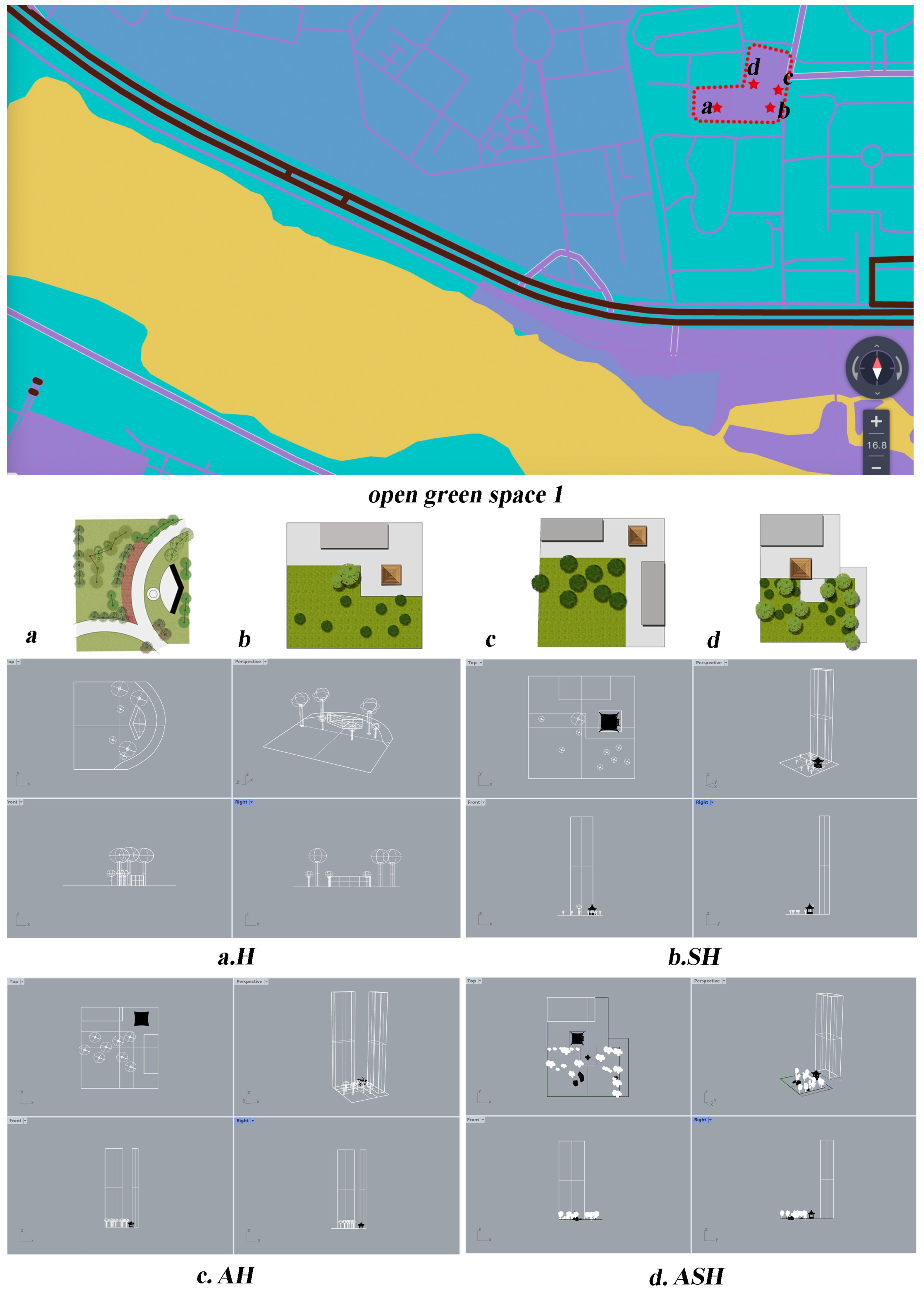
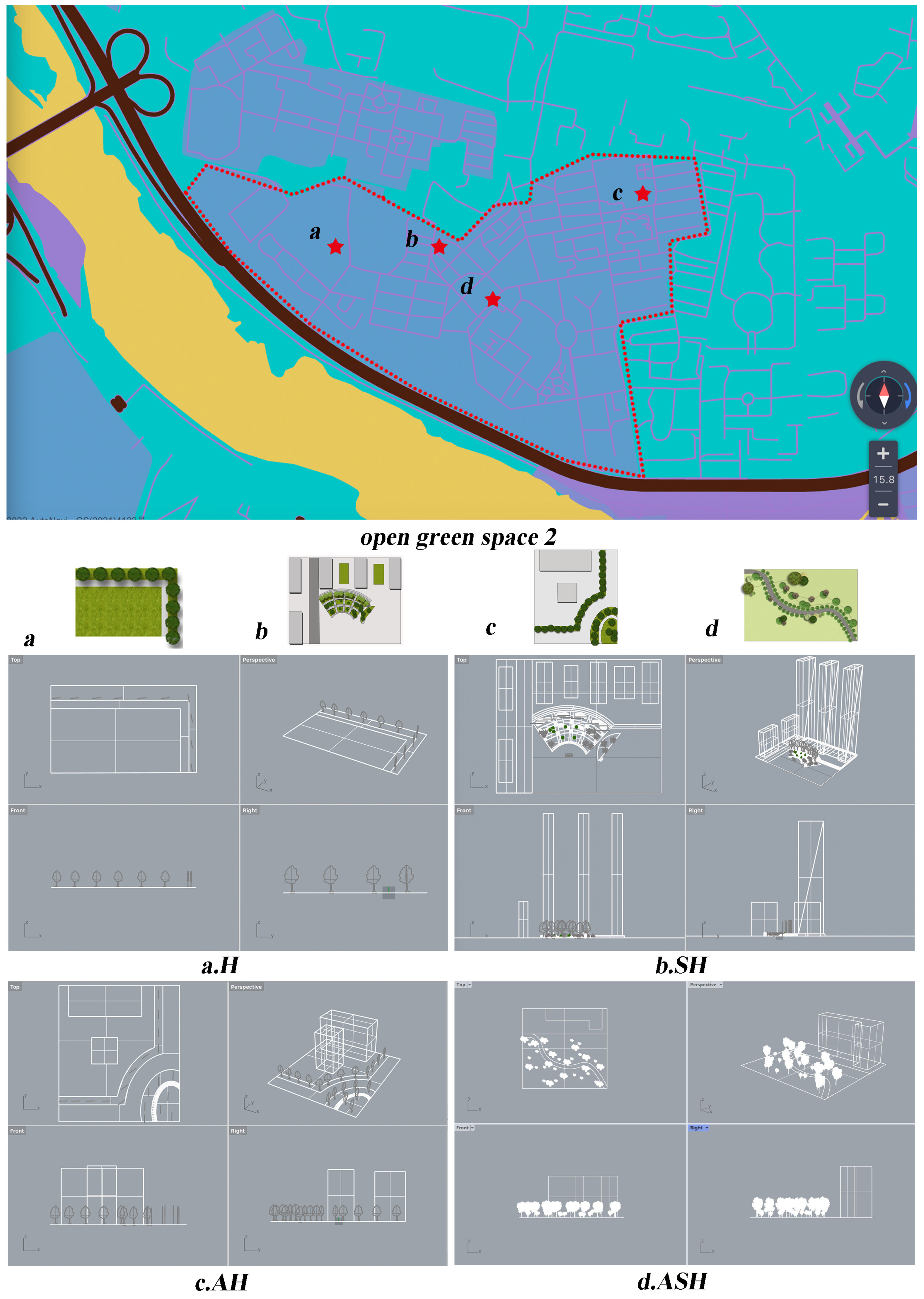
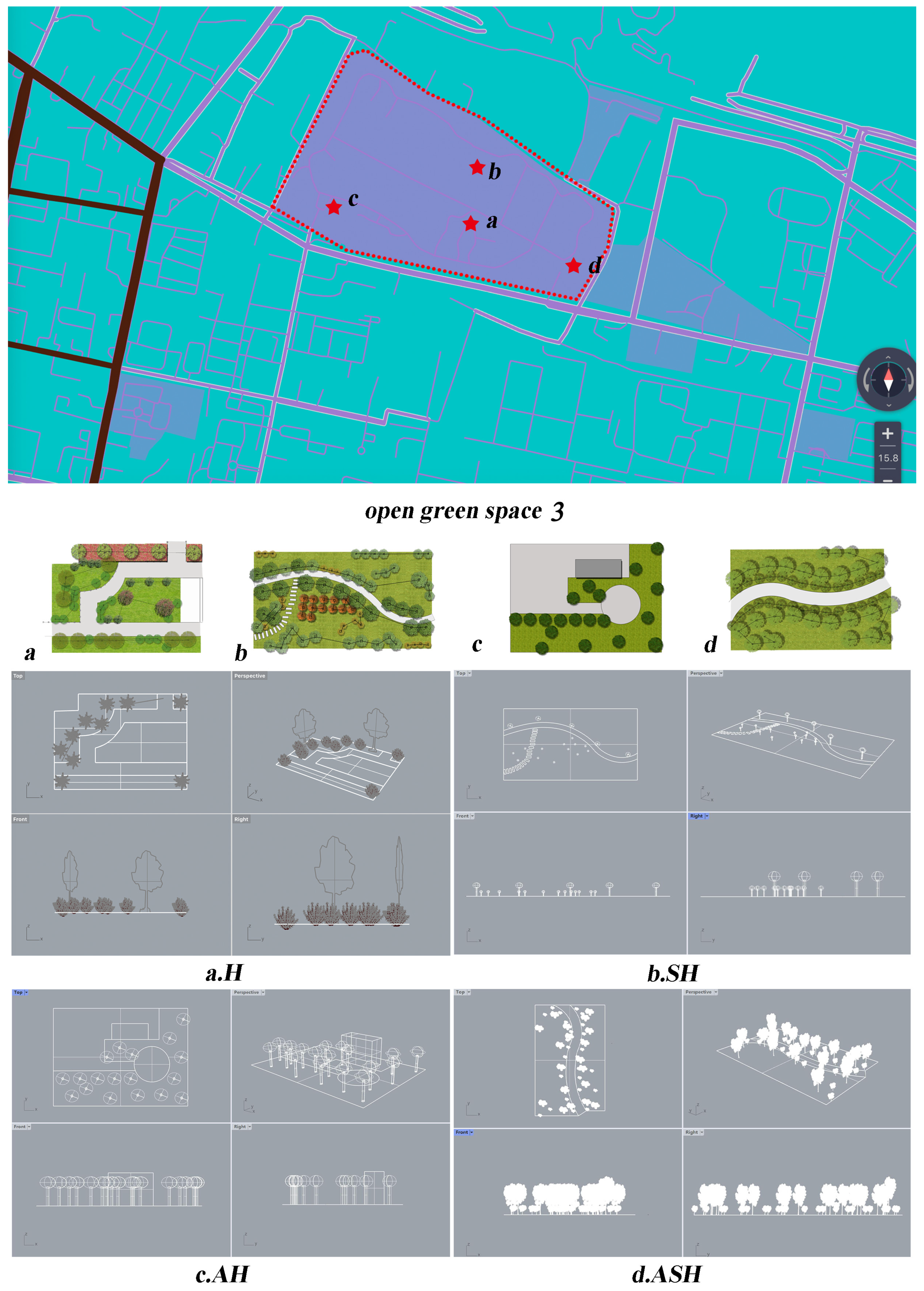
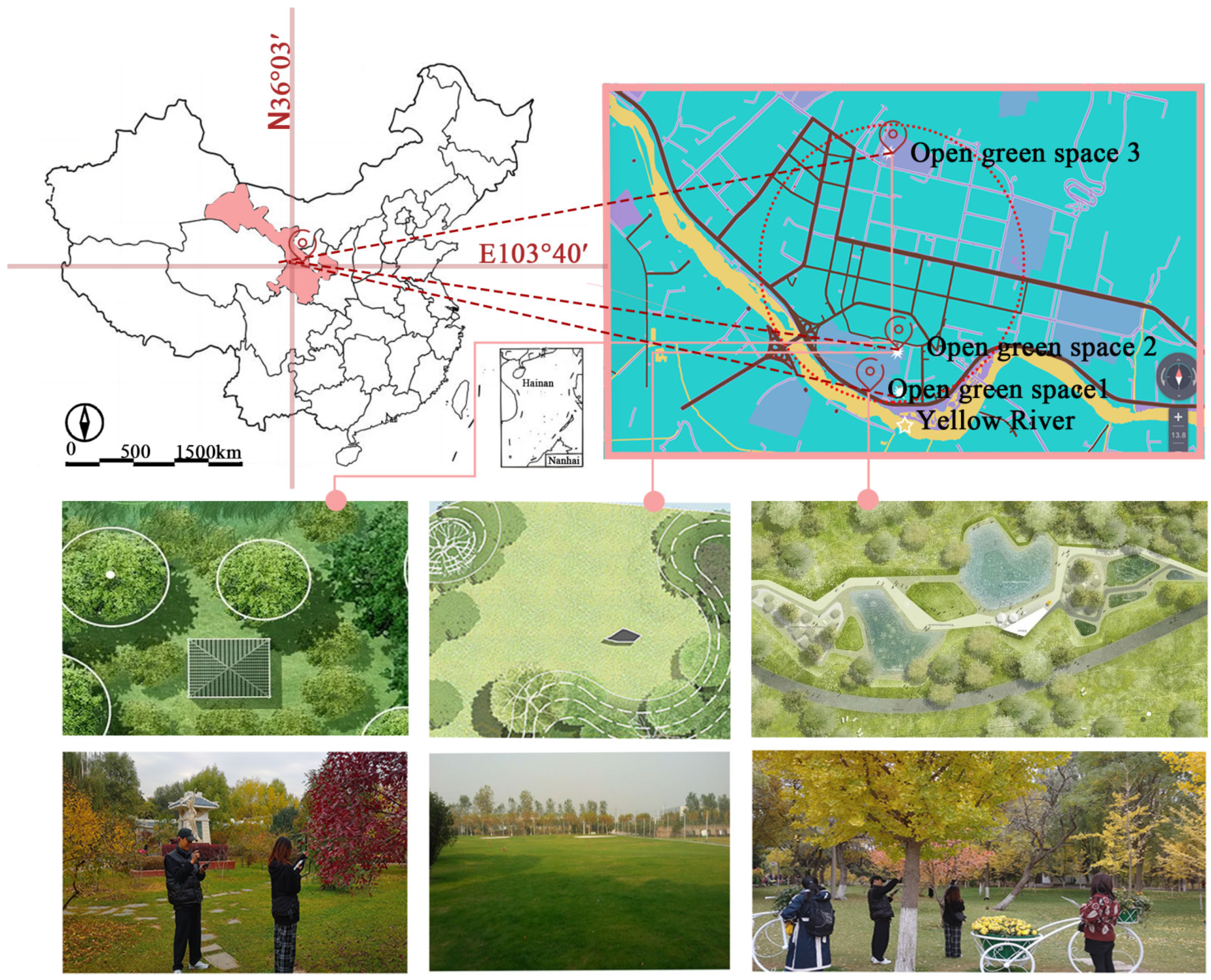
Lanzhou, as a river valley city in the northwest region of China, is characterized by low temperatures and strong winds. It is influenced by various factors such as terrain, geographical location, and monsoon [19]. These factors contribute to hot and windy summers, cold and dry winters, and a relatively low annual precipitation, resulting in an arid and cold climate in the city. According to meteorological data from Lanzhou for the period of 2001–2020 (CDCW, 2020), as shown in Table 1, the average annual temperature is mainly concentrated between 6 and 8 °C. The average annual relative humidity (RH) ranges from 55.0% to 61.0%. A field survey was conducted in a city park in Lanzhou, which is located at a longitude of 103°40′ E and latitude of 36°03′ N. The measured data for three sampling points are presented in Table 2. Among them, sampling point 1 is closest to the water, exhibiting a temperature difference of 10.7 °C between the maximum and minimum temperatures, with a relative humidity difference of 32.45. Meteorological parameters were measured on site, and the Ladybug Tools tool was utilized to calculate the Universal Thermal Climate Index (UTCI). Questionnaire surveys were conducted among visitors in these spaces to gather personal perception information and spatial perception intentions. The UEG (Urban Energy Game) tool was employed to predict spatial temperature and humidity changes on an hourly basis for one year. The Grasshopper tool was used to construct the spatial models, and the simulation and validation of thermal comfort environments were conducted using meteorological data and UWG (Urban Weather Generator) predictions for the three locations.
Table 1.
Average meteorological parameters in Lanzhou city from 2001 to 2020.
Table 2.
Measurement of spatial–temporal meteorological variables.
2.1. Study Site
Field investigations were conducted during the autumn (7 September and 8 December 2020) and winter (7 November and 7 December 2021) seasons, which corresponded to the coldest and driest periods in Lanzhou. The study areas were located in the Anning District of Lanzhou City, and various green open spaces at different distances from the Yellow River were selected for the investigation (Figure 1).
Figure 1.
Site locations and measured spaces.
2.2. Meteorological Measurement
Meteorological parameters, namely globe temperature (Tg), air temperature (Ta), relative humidity (RH), and wind speed (Va), were recorded every minute (Table 3). Tg was recorded using a WGBT-302, while Ta was measured using an anemometer. RH measurements were obtained using a SIGMA AS837 device [11]. In addition, Vv and Va were measured using a SIGMA AR866A thermal hand-held high-precision digital air volume test and measurement anemometer [14].
Table 3.
Technical details of meteorological equipment.
The study was conducted during the autumn and winter seasons with experimental observations taking place between 13:30 and 12:00. Measurements of various indicators were taken every 10 min, and the experiment was repeated three times to ensure accuracy. The study encompassed three distinct locations, and specific measurements were obtained from various spaces within each location, including grassland (H), shrub–grass (SH), arbor–grass (AH), and arbor–shrub–grass (ASH) spaces. More detailed information regarding the specific locations and spaces can be found in Appendix A Figure A1, Figure A2 and Figure A3, Tables S1–S4 .
The mean radiant temperature (Tmrt) was calculated on site in terms of the black globe temperature (Tg) and the air temperature (Ta) following the formula:
where (εg = 0.95) and (D = 0.05 m) are the globe emissivity and diameter, respectively.
The Universal Thermal Climate Index (UTCI) is a widely accepted parameter for measuring the thermal stress people experience when outdoors. The value of UTCI depends only on wind speed, average radiant temperature, relative humidity and actual air temperature. As calculating the UTCI equivalent temperatures by running the thermoregulation model repeatedly, calculations are performed via an extensive polynomial expression with 210 coefficients [16]. Calculations are performed via an extensive polynomial expression with 210 coefficients. The UTCI can also be calculated by the following simplified equation:
UTCI = 3.21 + (0.872 × Ta) + (0.2459 × Tmrt) − (2.5078 × Va) − (0.0176 × RH) (°C)
2.3. Questionnaire Surveys
Questionnaires were conducted simultaneously during the measurement of climatic factors such as wind speed (Appendix A). A total of 600 questionnaires were randomly distributed at 12:00 and 14:00 (±0.5 h) at the selected location with a total of 509 valid data. The survey questions were based on existing research and are set into three categories in this survey: the first was the personal information of each respondent, including age, gender, means of transportation and type of visitors (the thermal comfort questionnaire is an English translation from the original Chinese).
Part II of the questionnaire explored individual perceptions of different types of activities and thermal sensation, comfort and acceptability. Specifically, activity intensity preference was represented by a list of 5-level scales (low (1); lower (2); normal (3); higher (4); high (5)). Coming here for microclimate comfort was recorded on a 2-point scale (yes (0); no (1)). Specifically, thermal sensation was expressed by a list of 5-level scales (cold (1); cool (2); neutral (3); warm (4); hot (5)) (Appendix A).
Part III of the questionnaire surveyed strategies of microclimate and space improvement, including wind, humidity, sunshine, plant, architecture, waterscape and people. And it also explored people’s perceptions of the frequency of special weather (such as sandstorm, rainstorm, hail, extreme drought and extreme low temperature). Frequency was represented by a list of 5-level scales (many (1); more (2); general (3); less (4); few (5)). (Appendix A).
2.4. Presentation of the Simulation Workflow in Grasshopper
The initial step involved in this study was to procure a suitable weather dataset from available sources in “epw” format, which is widely compatible with a variety of simulation tools. And the authors selected the full year data for the study time based on the “.epw” format data. The Urban Weather Generator (UWG) is a tool utilized in this study, which is designed to estimate urban canopy air temperature and relative humidity on an hourly basis. To achieve this, it takes into consideration various factors such as heat exchange and air stratification in different atmospheres [20,21]. The parameters used in the study include Va, RH, Ta, Tg, Sunshine (Ss), and UTCI, which were obtained from a 3D model of the study area, which was constructed using Rhinoceros. These values were considered to be representative of the urban scale, and were easily incorporated into the workflow using the graphical interface provided by the Ladybug tool within the Grasshopper environment. This enabled seamless integration with other components of the proposed workflow.
In the final part, the Ladybug tool was employed to simulate the primary influence of wind elements on the environment. Approaches available in Grasshopper include wind analyses using Butterfly [11] or Eddy3D [14] which produce wind factors, the ratio between the simulated wind speeds and the inlet wind speed generated from a number of directions. In this study, Ladybug in Grasshopper was found to be faster, more accurate, and suitable for wind analysis. The workflow diagram for the development and testing of Ladybug is shown in Figure A1, highlighting the connections between different tools. The first step of the proposed simulation workflow was to create an appropriate geometric representation of the urban area under study.
3. Results
3.1. Deceptive Analysis
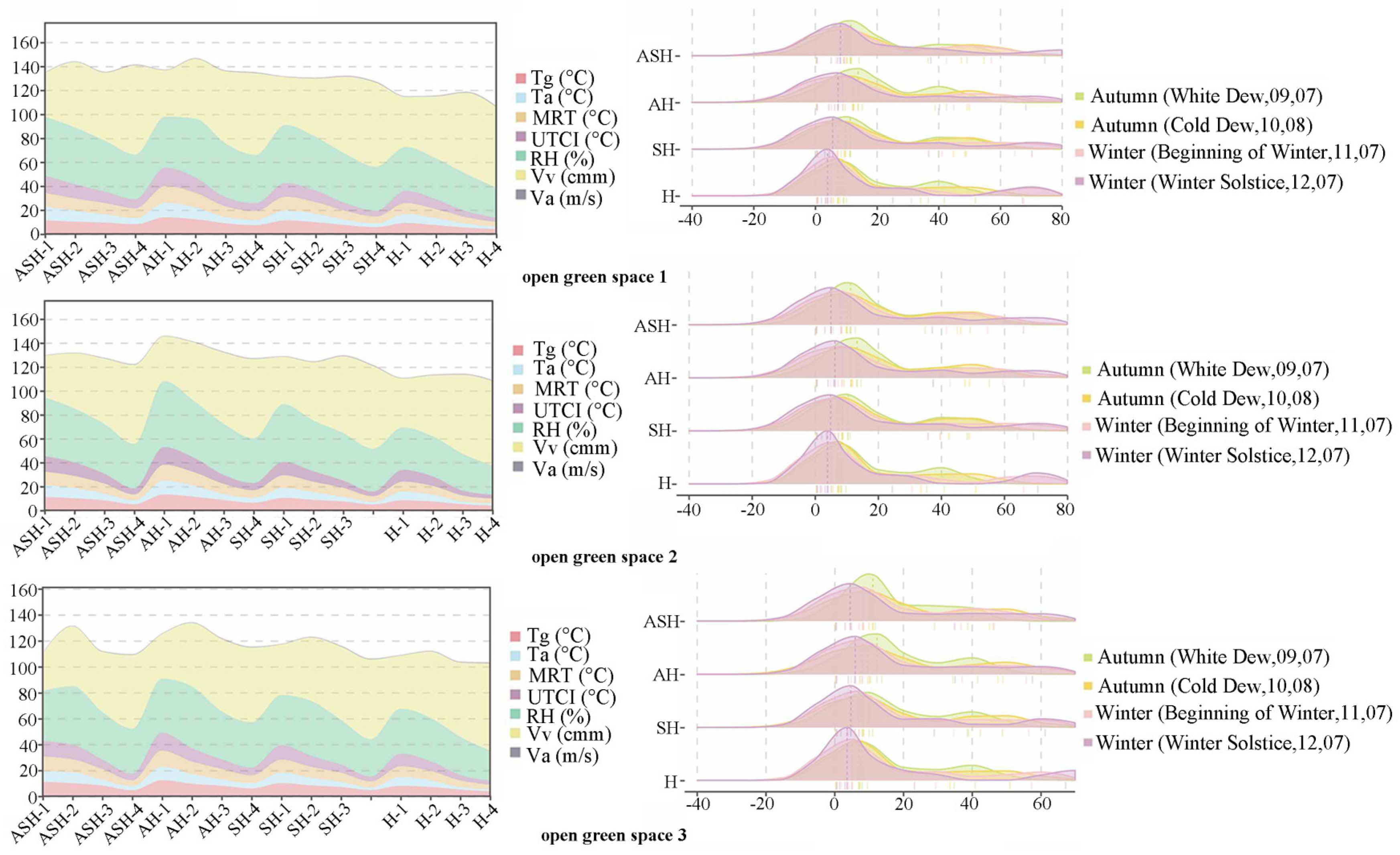
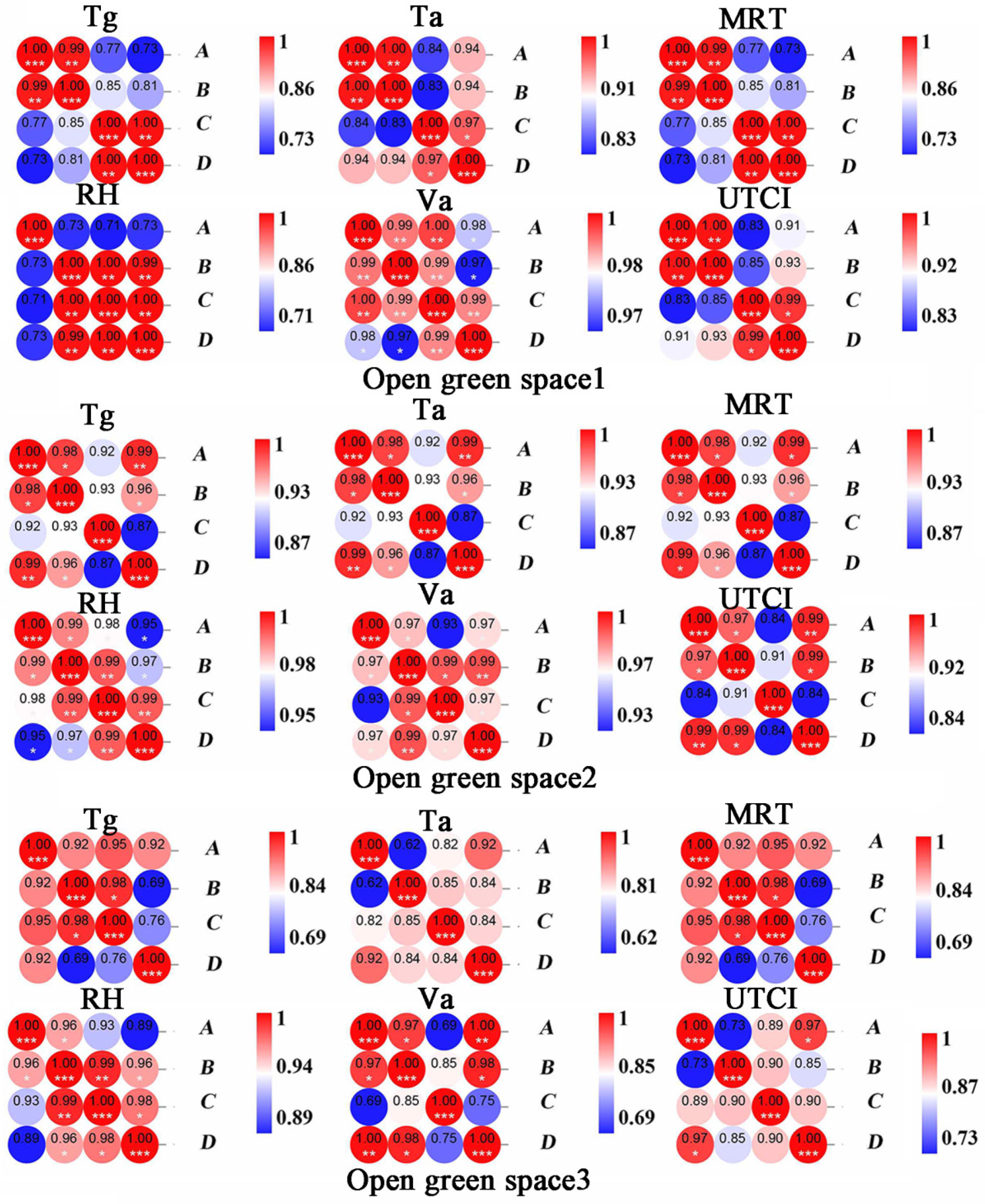
3.1.1. Measured Meteorological Parameter
Meteorological variables of 10 species of single arbor (A) and single shrub (S) measured during autumn and winter are listed in Appendix B. Va, Vv of A, S, Ta, Tg and RH all increased significantly. Based on onsite meteorological measurements and field surveys of plant communities, it has been observed that Cornus chinensis and Ligustrum lucidum are dominant tree species in the local area. Their robust branches and dense foliage contribute to their strong wind resistance, enabling them to effectively withstand strong winds [22]. Picea asperata exhibits the strongest thermal insulation due to its needle-like structure. Ilex rotunda, with its thicker wax-coated leaves, helps reduce water loss, resulting in its strong moisturizing ability.
Meteorological variables of the four planting patterns measured during autumn and winter are listed in Appendix A. The order of cooling ability of the four planting patterns was arbor and grass (AH) > arbor–shrub–grass (ASH) > shrub–grass (SH) > grass (H). The order of moisturizing ability of the four planting modes was AH > ASH > SH > H. It shows that the shrub has a certain humidification effect, but it is smaller than that of the arbor. The order of wind resistance of the four planting modes is ASH > AH > SH > H. Because of the wind-blocking ability of shrubs, AS and ASH had the strongest wind-blocking ability. H had the weakest wind-blocking effect, and the grass hardly affected the air flow at the pedestrian level. Through the analysis of dynamic Stream Chart and dynamic Ridgeline plots, the Va and Vv of the three OGSs increased significantly with the seasons, while the Ta, Tg and RH decreased significantly with the seasons. In the three OGS, RH, Va and Vv decreased significantly with the distance from the Yellow River, while Ta, Tg, MRT and UTCI increased significantly (Figure 2). Significant differences in meteorological variables among the three spaces and the four planting patterns were determined through post hoc Tukey tests (Figure 3). The Va near the Yellow River for two OGSs was significantly different in winter and autumn (p > 0.05). The RH of all three OGSs was significantly different in winter.
Figure 2.
Dynamic Stream Chart and dynamic Ridgeline plots. The X-axis of the three graphs on the left represents “the sampling point numbers of the Qiaoguan grass”, while the Y-axis represents “Globe Temperature (°C), Air Temperature (°C), Mean Radiant Temperature (°C), Universal Thermal Climate Index, Relative Humidity (%), Velocity of Air Motion (cmm), and Air Velocity (m/s)”. The X-axis of the three graphs on the right represents the four seasons, while the Y-axis represents “the sampling point numbers of the Qiaoguan grass”.
Figure 3.
A post hoc Tukey’s test for different pairs of measurement points for the meteorological variables (ASH, AH, SH and S). A–D stand for different times, 09,07, 10,08, 11,07, 12,07; * p < 0.05 ** p < 0.01. (*** is the significance difference analysis, the more * the more significant the difference).
3.1.2. Respondent Attributes
A total of 509 effective questionnaires were collected, including 166 in OGS1, 148 in OGS2 and 195 in OGS3. Respondents were composed of 50.69% females and 49.31% males, 22.40% seniors (>55 years old), 67.78% adults (18–55 years old) and 9.82% children (<18 years old). In trials, the majority of respondents reported intensity perceptions for different activity types and perceptions of comfort in different spaces (Figure 4 and Figure 5). At the same time, the perception of Lanzhou’s special weather and suggestions for space renovation were also reported for respondents.
Figure 4.
The comfort level of respondents in different spaces.
Figure 5.
Respondents’ perception of extreme weather in different spaces.
1. Effects of physical factors
Among physical factors, the effects of Ta, RH and Va on the thermal perception of the human body were considered [23]. In this study, all meteorological parameters influenced the thermal sensation of respondents. In OGS1, Va had the highest correlation with thermal sensation among respondents, followed by Ta and RH then G in order. In OGS2, Ta and RH had the highest correlation with thermal sensation among respondents, which was followed by Va and then G in order. In OGS3, Ta and RH had the highest correlation with thermal sensation among respondents, which was followed by Va and then G in order.
2. Effects of individual factors
Among individual factors, effects of age, gender, and activity level on the thermal perception of individuals were considered [22]. In this study, there were effects of individual factors on thermal microclimate comfort for respondents. In OGS3, the thermal comfort of microclimate for respondents was influenced by personal activities. The mode of transportation had a negative impact on perceptions of comfort.
3. Landscape elements
In this study, people’s perceptions of the comfort of small environments such as squares, trees, lawns, roads, watersides, buildings, etc. were interviewed by the authors (Figure 6). Discovered by analysis, the comfort of grass space for respondents is affected by the gender in OGS1. The comfort of the waterside is affected by activity. In OGS2, the comfort of grass space for respondents was affected by the Ta and RH. The comfort of architecture was affected by the gender. In OGS3, landscape elements did not have a statistically significant effect on respondents’ comfort level.
Figure 6.
Respondents’ opinions on renovation of different spaces.
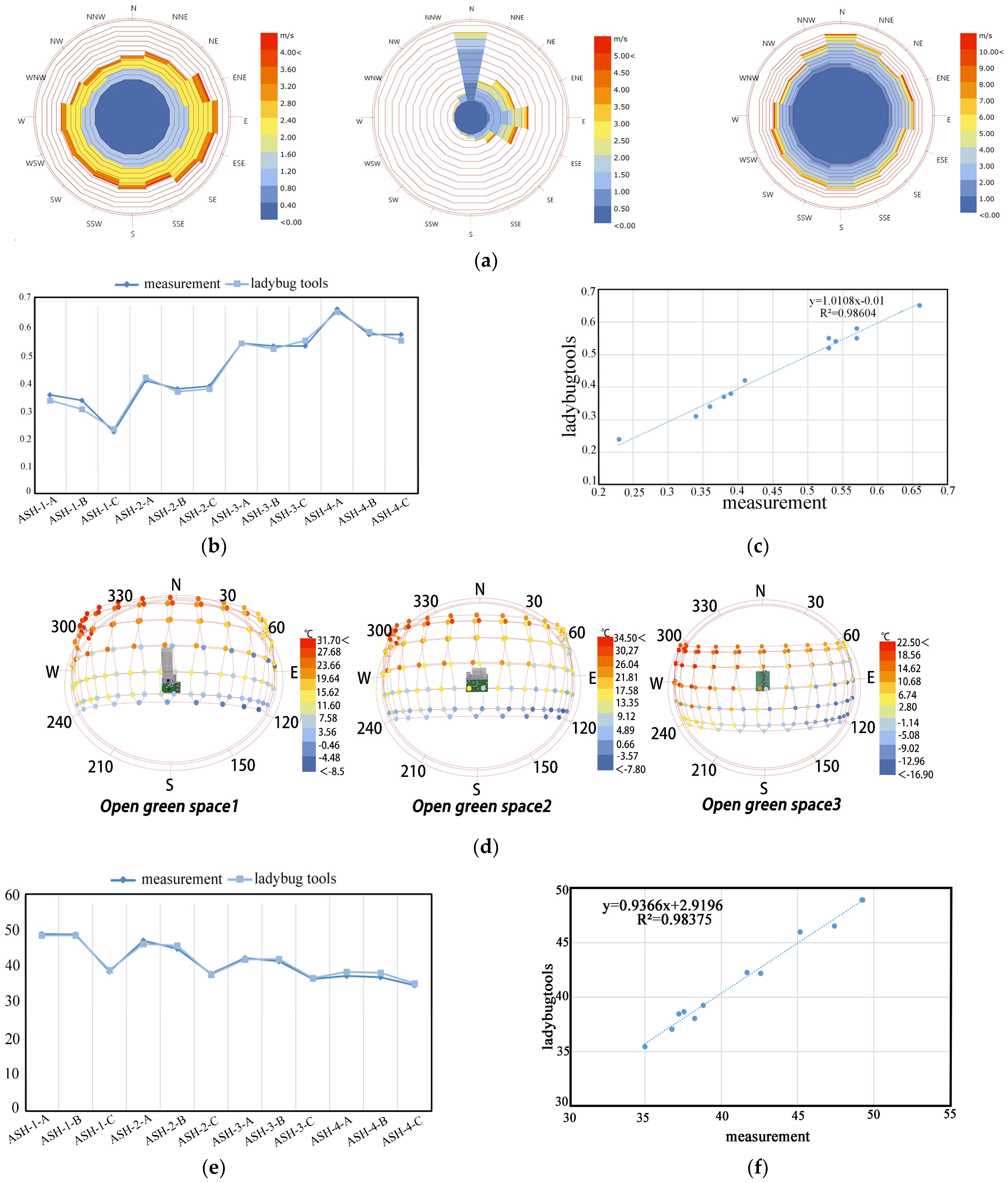
3.1.3. Va and RH Simulation in the Model
To validate the reliability of the Ladybug tool in calculating outdoor relative humidity and wind speed, probes were used to apply the same profiles of relative humidity and wind speed within self-built models. The simulated temperature and humidity results for the three spaces were obtained. Wind speed (Figure 7a) and relative humidity (Figure 7c) are simulated through three green space models. It can clearly be seen that although the parameters Va and RH have some discrepancies with the measured values, the fitting degree is high and there is consistency (Figure 7b,e). The results show that there is a strong positive correlation between different spatial measurements and model outputs Va and RH, R2 = 0.986 (Figure 7c), R2 = 0.984 (Figure 7f). It can clearly be seen that although the parameters Va and RH have some discrepancies with the measured values, the fitting degree is high and there is consistency. The results show that there is a strong positive correlation between different spatial measurements and model outputs Va and RH, R2 = 0.986, R2 = 0.984 (Figure 7a–d).
Figure 7.
(a) Wind speed simulation results. (b) Relationships between measured and simulated Va. The X-axis represents the sample point number, while the Y-axis represents air velocity. (c) Simulation results of air velocity. (d) Relationships between measured and simulated RH. (e) Relationships between measured and simulated RH. The X-axis represents the sample point number, while the Y-axis represents relative humidity. (f) Relative humidity simulation results.
3.1.4. UTCI Simulation in the Model
It can be clearly seen that the parameter UTCI is in good agreement with the field measurements. The results show that the Ladybug Tools workflow simulates the thermal performance of the geometric configuration with considerable reliability and a short simulation time. Therefore, it can be used for the environmental simulation of the studied locations in this research. The simulation results represent the temperature variations for each hour of every day throughout the year for the three spaces. Although there is some discrepancy between the UTCI parameter and the measured values, there is a high level of fit and significant consistency with an R-squared value of 0.936 (Figure 8).
Figure 8.
Relationships between measured and simulated UTCI.
3.1.5. Implications for Designers
In Lanzhou, due to the cold lake effect of the Yellow River, the outdoor thermal perception of scenic open spaces was mainly influenced by wind. Therefore, it was a great opportunity to improve outdoor comfort by implementing an optimized design of landscape features. Through the joint verification of actual measurement and simulation, it was concluded that in order to cope with the low temperature and minimum precipitation in the autumn and winter seasons, tree species with strong insulation and moisture retention capabilities should be given priority consideration in the design. At the same time, the analysis revealed a negative correlation between activity levels and respondents’ thermal comfort, emphasizing the importance of providing comfortable activity spaces in design. In addition, our simulation results indicated that there was an important connection between an individual’s thermal adaptation ability and the spatial environment. These results were further elaborated in Table 4 and Figure 9. Research on the thermal comfort of grouped and single plants indicated the following microclimate comfort levels: ASH > AH > A and A > S > H (Figure 9a).
Table 4.
Bioclimatic design strategies suitable for scenic open spaces in urban areas.

Figure 9.
Schematic diagram of bioclimatic transformation.
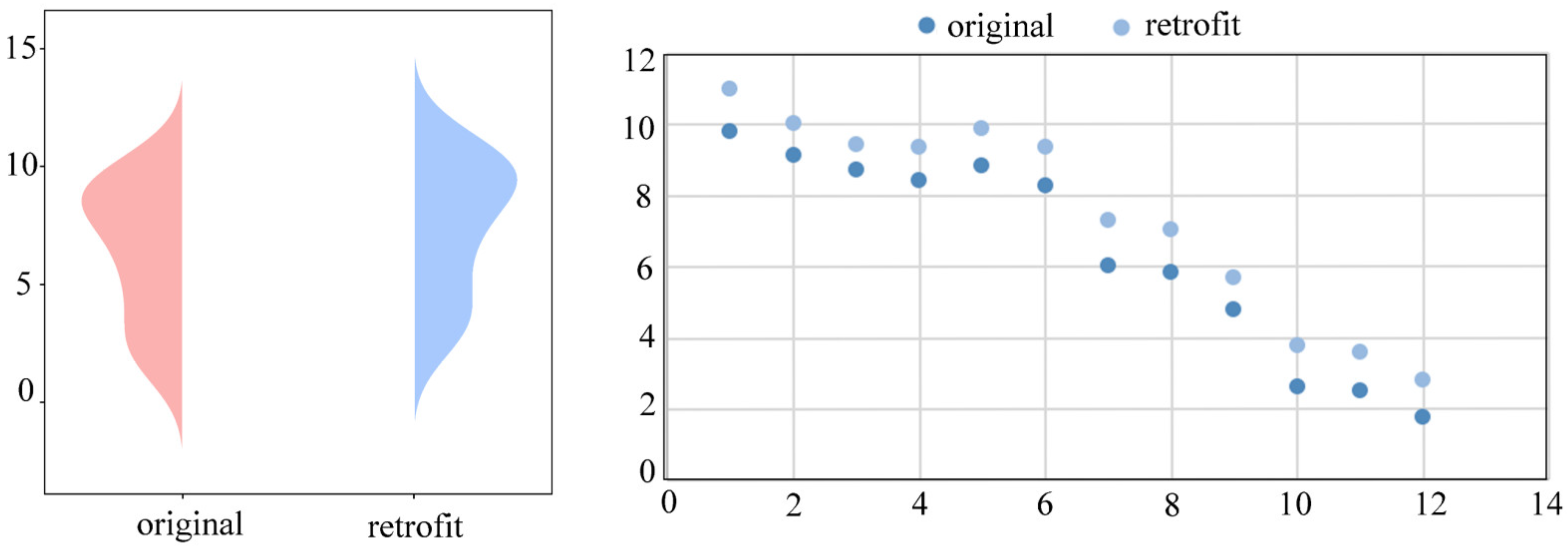
3.1.6. UTCI after Retrofit
In order to investigate the effects of snowstorm, wind volume, wind speed, temperature, relative humidity and solar radiation on the thermal comfort of small environments, three open green spaces models were established using Rhino (Figure 9). The results show that the Ladybug Tools workflow simulates the thermal performance of the geometric configuration with considerable reliability and a short simulation time; therefore, it can be used in this study. Three open green spaces (ASH) were transformed to simulate comfort after modeling. It was found that the UTCI values were higher than before the transformation (Figure 10). By utilizing the Ladybug tool, simulations were conducted for three open green spaces. Six different perspectives were captured within the software to calculate the Universal Thermal Climate Index (UTCI) for the developed models of these three open green spaces. The x-axis represents the months from January to December, while the y-axis represents the UTCI values. From the graph, it is evident that the red areas are predominantly concentrated in July and August, indicating that the optimal thermal comfort is mainly observed during these two months. Furthermore, the comfort levels among the three open green spaces are comparable, indicating that the renovation efforts can alleviate the heat island effect (Figure 11). In addition, the authors simulated the site sunshine through the model. According to Figure 12, the legend indicates the UTCI values, where colors closer to red represent higher UTCI values, while cooler colors indicate lower UTCI values. It was found that the Ss values of the three green spaces were not much different, which was consistent with our conjecture (Figure 12).
Figure 10.
Compare original and retrofit UTCI.
Figure 11.
UTCI simulation result.
Figure 12.
Retrofit sunshine.
4. Discussion
4.1. Factors Affecting Thermal Comfort
Due to the prominent winter microclimate problems in northern China, Lanzhou is cold and long in winter and cools down quickly in autumn. The research is discussing the relationship between different plant configuration patterns and the local microclimate environment in open green spaces at different distances from the Yellow River, which is mainly for the analysis and research of the measured climatic conditions in autumn and winter.
4.1.1. Physical Factors
The present study evaluates the efficacy of different plant configurations in creating environmental comfort. Specifically, it is found by the authors that when a single plant type is employed, trees have the greatest potential to enhance thermal comfort conditions. On the other hand, composite structure types, such as arbor and grass combinations, exhibit the most significant impact on cooling and humidity. Furthermore, the combination of arbor, shrub and grass is found to be most effective in terms of average wind speed and wind-blocking ability in urban green spaces. Notably, our research supports the notion that dense tree coverage is conducive to mitigating heat stress, although vegetation may negatively affect wind ventilation [23,24]. Moreover, our study reveals that changes in relative humidity (RH) are inversely proportional to mean radiant temperature (MRT) and ambient temperature (Ta) during the winter solstice, which is the coldest season in Lanzhou. This finding is consistent with prior research that has shown that the cold lake effect of the Yellow River significantly influences wind conditions in the region during winter [25]. In addition, the authors observed that in OGS1, the thermal sensation of the respondents was most closely related to the air velocity (Va), indicating the significant impact of the UHI (cold lake effect) [26], which is a climatic phenomenon commonly observed in river valley cities at middle to high latitudes. Conversely, on OGS2–3, thermal sensation was most closely correlated with Ta and RH, followed by Va, suggesting that these meteorological factors play a crucial role in influencing thermal perception. Therefore, our results highlight the importance of considering strategies to manipulate Va during the design of outdoor spaces [27].
4.1.2. Individual Factors
The perception of thermal thresholds is influenced by various demographic factors, such as age, gender, and test site [28,29]. However, the present study did not identify any significant effects of individual factors (age and gender) on the thermal microclimate comfort of the respondents. Nevertheless, there were discernible differences in comfort levels across the various test sites. The thermal comfort of respondents in OGS1–2 was not associated with individual factors. However, in OGS3, the thermal microclimate comfort of respondents was found to be influenced by their activity levels. Specifically, the respondents’ mode of transportation to the test site was observed to negatively impact their perception of comfort. This could be attributed to the location of OGS3 on the outskirts of the city, far from the Yellow River, which required respondents to undertake a high level of activity to reach the test site [30].
4.1.3. Environment Factors
The impact of high-rise buildings on microclimate has been well documented in the literature [30]. In the present study, gender was found to influence architectural comfort in OGS1, which is consistent with the fact that this site has the highest number of high-rise buildings among the three test sites. Microclimate perception within the enclosed space of high-rise buildings was found to be inconsistent. A study conducted in Changsha, China, investigated the microclimate of two public squares and explored the effects of buildings, trees, water, and landscape design on improving thermal comfort [31,32]. Within our study, significant differences in respondents’ perception of comfort in grass spaces were observed within OGS2. In OGS1, thermal and humidity factors (Ta and RH) were found to influence comfort in grass spaces. However, the dry and cold climate during autumn and winter may not provide adequate improvement in environmental temperature and humidity within the open grassland spaces [33].
4.2. Microclimate Simulation Parameters
The ladybug tool model was chosen for this study to simulate micro environmental climates for several reasons: it is considerably less time consuming to perform calculations, allowing for the simulation of climatic factors for various plant configurations, including RH, Ta, Tg, Va, Sunshine and UTCI, which are focus on this study, and the ability of parameterization model various spatial shapes, and visualize the results in the Grasshopper environment.
The Ladybug Tools model was selected to simulate micro-environmental climates for several reasons. Firstly, it allows for the simulation of climatic factors for various plant configurations, including relative humidity (RH), air temperature (Ta), globe temperature (Tg), wind velocity (Va), sunshine, and Universal Thermal Climate Index (UTCI), which are the focus of this study. Secondly, the Ladybug Tools model considerably reduces the time required to perform calculations. Thirdly, it enables the parameterization of various spatial shapes and visualization of the results in the Grasshopper environment.
The Ladybug Tools model is a combination of Grasshopper plugins that estimate outdoor thermal comfort through graphical representation. The model connects Grasshopper to proven software engines that individually calculate thermal comfort determinants. For instance, Honeybee links Grasshopper with EnergyPlus [34] to calculate surface temperatures, while Dragonfly uses the Urban Weather Generator (UWG) [19] to calculate urban air temperature and relative humidity. In this study, Lanzhou city’s weather data in “epw” format was used, and the Ladybug component was used to visualize environmental data and output results. The simulations of Tg, Ta, and RH were compared with measured results, which demonstrated strong correlations of R2 = 0.996, R2 = 0.997, and R2 = 0.984, respectively. Although the Butterfly plugin could integrate Open FOAM software (OpenFOAM 9) for computational fluid dynamics (CFD) air-flow analysis, it requires significant computation time. Therefore, the wind speeds in this study were retrieved from weather files, which still demonstrated a strong correlation of R2 = 0.986.
The present study employs a rigorously validated software engine to determine the mean radiant temperature (MRT) and thermal comfort components. In this study, weather data for Lanzhou city in “epw” format was used, and the Ladybug component was employed to visualize the environmental data and output results. The simulation results of Tg, Ta, and RH were compared with the measured values, showing strong correlations with R-squared values of 0.996, 0.997, and 0.984, respectively. The Urban Weather Generator (UWG) has been validated through field measurements in diverse climates [19,20] and is utilized to investigate how different UTCI components are combined and how the MRT equations are applied, both of which require validation. In a Mediterranean climate context, Evola et al. validated the Ladybug Tools workflow through experimental measurements of MRT in Catania, Italy [35]. Their study reported a coefficient of determination R2 = 0.92 in good agreement with measurements. Additionally, the present study rigorously validates the workflow implemented in Ladybug Tools modeling. As shown in Figure 2, the average UTCI results for all three open green spaces exhibit consistent performance with an R2 of 0.936. This indicates that the proposed method exhibits good reliability in scenarios with the cold lake effect in middle to high-latitude regions. In similar environmental settings, this simulation can be applied in the early design process to model and assess alternative schemes, aiming to find space design solutions that offer improved thermal comfort while fulfilling other functional requirements. Subsequently, the design can be further refined and implemented during construction.
4.3. Retrofit Strategy
In this paper, through the actual measurement and simulation verification of different vegetation configurations in different open green spaces at different distances from the Yellow River, the design strategy with the best environmental comfort is found. The methodology described in this paper can be replicated and used to test other performance criteria, such as energy loads, through its core simulation engine, EnergyPlus [36]. Grasshopper is very friendly to planners, designers and others without proficiency in programming. There is no doubt that the use of open source plugins and environment plugins in Grasshopper has increased its popularity in climate research and has quickly become an indispensable tool in practice [37]. The method described in this article can be replicated and used to test other performance standards, such as energy load, by utilizing its core simulation engine, EnergyPlus [38].
A comprehensive approach was taken to evaluate the impact of different vegetation configurations on environmental comfort in various open green spaces situated at varying distances from the Yellow River. The methodology outlined in this research can be replicated and extended to examine other performance criteria, such as energy loads, through its core simulation engine, EnergyPlus. Grasshopper, with its open source and environmental plugins, has emerged as a popular and user-friendly tool for planners, designers and researchers without expertise in programming [18]. Our study establishes a close correlation between the Tg, Ta, Vv and RH measurements and simulation results. A visual tool, the “UTCI Rose”, was developed by the authors to analyze people’s perceptions of the comfort of small environments and guide urban designers in creating comfortable outdoor environments. The UTCI values reported in our study provide a direct measure of pedestrian thermal comfort in degrees Celsius, thereby facilitating the incorporation of climate indicators into design guidelines at different scales from districts to small urban areas. The methodology outlined in this study has the potential to contribute to the creation of resilient and sustainable urban environments that ensure pedestrian comfort.
4.4. Limitations
The wind and humidity analysis was performed based on the wind speed and relative humidity in the file, as these variables exhibited high reliability in the workflow. While other methods such as wind analysis using Butterfly or Eddy3D [15] are available in Grasshopper and generate wind factors that simulate wind speed in many directions, they are not as accurate as accounting for turbulent heat exchange in the model, which is a feature in the Open FOAM software currently under development and not yet integrated into either of the two plugins. Additionally, the Ladybug Tools model was found to underestimate the UTCI by approximately 3.5 °C compared to the field measurements, which was mainly due to spatial resolution issues in the plant simulation model that may lead to inaccurate sun occlusion angles. Despite these differences, they remain consistent under hypothetical cases and are thus acceptable. However, the model requires further refinement for detailed analysis.
5. Conclusions
In this study, a comparison of respondents’ perceptions of the thermal environment was conducted in three different types of sites in Lanzhou, China, utilizing different plant configuration spaces. Through the use of meteorological measurements and questionnaires, the physical, personal, and environmental factors that influence the thermal perception of residents and tourists were systematically discussed and compared. The study drew some major conclusions:
- (1)
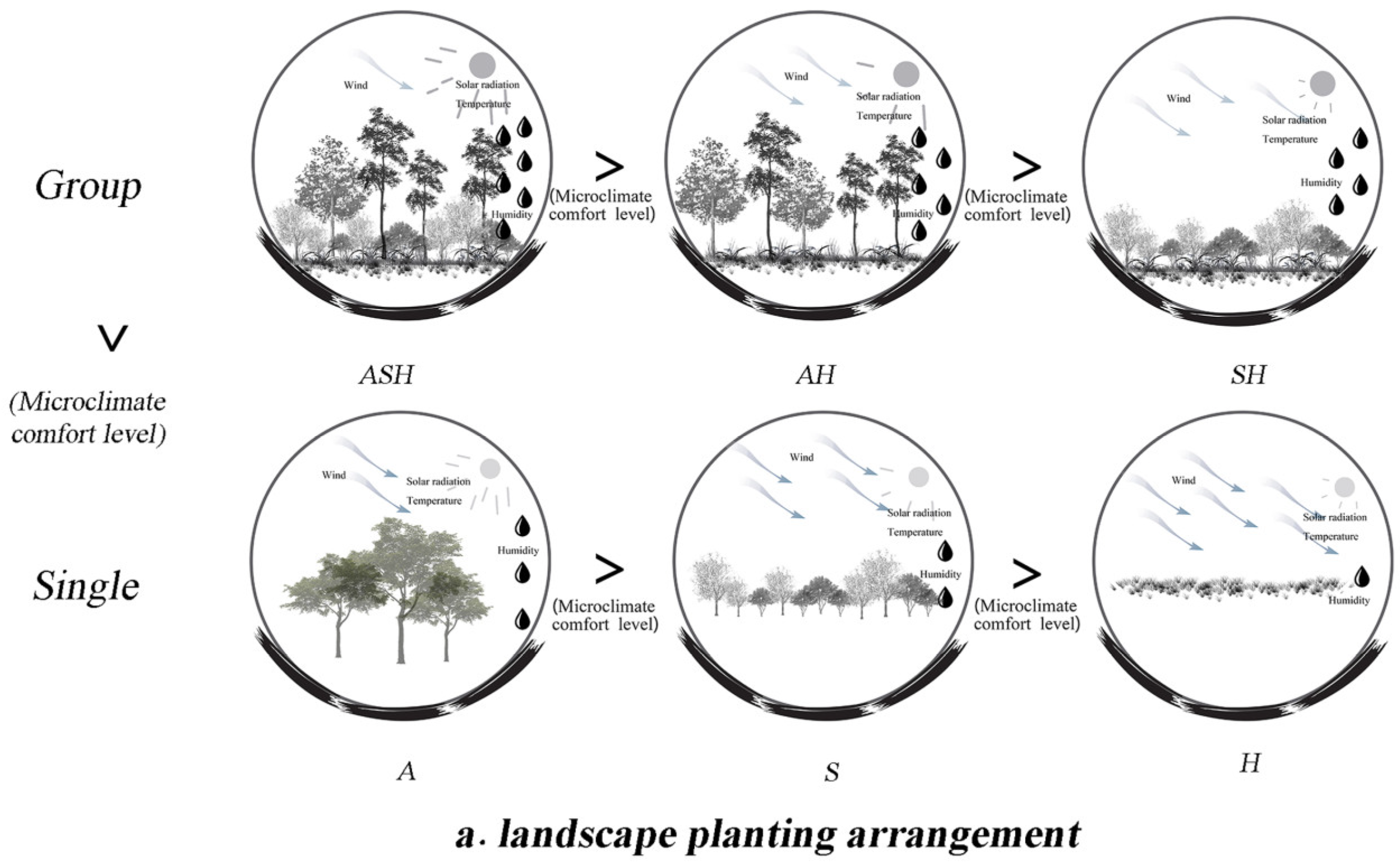
- The cooling ability of the four planting patterns was ranked in order of arbor and grass (AH) > arbor–shrub–grass (ASH) > shrub–grass (SH) > grass (H), while the moisturizing ability was ranked in order of AH > ASH > SH > H, and the wind resistance was ranked in order of ASH > AH > SH > H. The values of air velocity (Va) and vertical air velocity (Vv) increased significantly with seasons in the three spaces, whereas air temperature (Ta), ground surface temperature (Tg), and relative humidity (RH) changed significantly with seasons in the three spaces. Secondly, the change of RH was found to be inversely proportional to the solar radiation (SR) and mean radiant temperature (MRT), and the RH during winter solstice was the smallest in autumn and winter.
- (2)
- The cold lake effect of the Yellow River dominates the wind environment in Lanzhou, and the wind speed in winter is high. In OGS1, Va had the highest correlation with respondents’ thermal sensation. The residential area is closest to the Yellow River, indicating that the cold lake effect of the Yellow River does cause strong winds in the environment, which has a certain impact on comfort. In OGS2–3, Ta and RH had the highest correlations with thermal sensation among respondents, which were followed by Va and G.
- (3)
- The present study highlights the influence of individual factors on respondents’ thermal microclimate comfort with notable variations across different sites. Specifically, in OGS2, respondents exhibit significantly diverse perceptions of the comfort of grassy spaces on the campus. In OGS1, gender affects the comfort of buildings, whereas the comfort of grass space is influenced by Ta and RH. Conversely, individual activities have a significant impact on respondents’ thermal comfort in OGS3.
- (4)
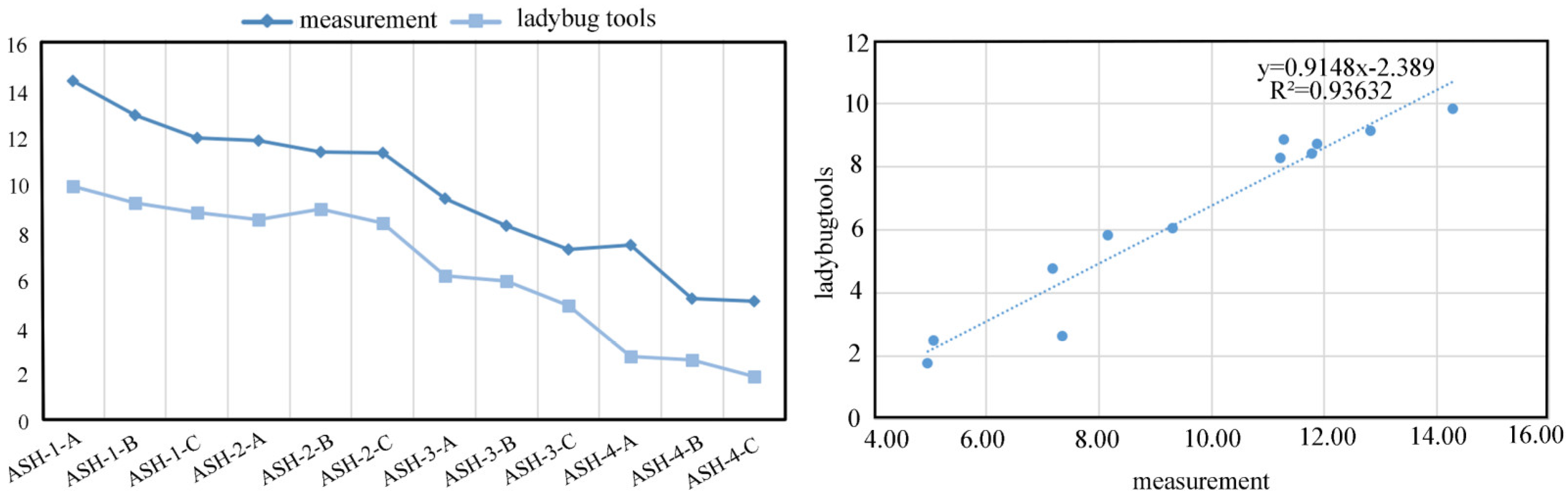
- Despite certain discrepancies between the measured values and UTCI parameters, the high degree of consistency and good fitting degree, R2 = 0.936, indicate that the parameters Tg, Ta, Va, and RH exhibit good agreement with the field measurements, with R2 values of 0.996, 0.997, 0.986, and 0.984, respectively.
The findings of this study provide insight into the mechanism underlying respondents’ thermal perception of the cold lake effect associated with the Yellow River. Furthermore, the site and actual measurement were simulated by the authors using Ladybug Tools, and the renovation plan was verified to achieve people’s thermal comfort. The implications of our results and methodology are expected to provide theoretical guidance for urban planners to consider climate-responsive design principles such as vegetation, irrigation, and shading to enhance outdoor comfort for visitors. The high level of fit between the simulated and measured data also indicates the reliability of this method in similar environments. It can be used as a reference in the early stages of design to assess and optimize the thermal comfort of spaces.
Supplementary Materials
The following supporting information can be downloaded at: https://www.mdpi.com/article/10.3390/buildings13092329/s1. Table S1. Volunteers’ attributes. Table S2. Open green space 1. Table S3. Open green space 2. Table S4. Open green space 3.
Author Contributions
Conceptualization, J.L. and S.J.; methodology, J.L.; software, S.J.; validation, S.Z. and S.Y.; formal analysis, S.Z.; investigation, W.J.; resources, W.J.; data curation, J.L.; writing—original draft preparation, J.L.; writing—review and editing, J.L. and S.J.; visualization, S.J.; supervision, W.L.; project administration, W.J.; funding acquisition, W.J. and W.L. All authors have read and agreed to the published version of the manuscript.
Funding
This research was funded by the Ministry of Science and Technology of China (2019FY101604).
Data Availability Statement
The data presented in this study are available on request from the corresponding author.
Conflicts of Interest
The authors declare no conflict of interest.
Appendix A
Thermal comfort questionnaire (English translation from the original Chinese).
- 1.
- Location: ______ Time: ______ Length of time living locally: ______ Hometown: ______ Current wind speed: ____________ Current temperature/humidity: ____________Current sunshine: ____________ (1, 2, 3 and 4, four levels are enhanced in turn)
- 2.
- Gender: _________ Age: _________ Occupation: _________
- 3.
- Means of Transportation: ( ) A. Self-driving B. Bus C. Subway D. Taxi E. Shared bike F. Walking
- 4.
- Activity type and perceived intensity
| Low | Lower | Normal | Higher | High | |
| Sitting | ○ | ○ | ○ | ○ | ○ |
| Standing | ○ | ○ | ○ | ○ | ○ |
| Slow walking | ○ | ○ | ○ | ○ | ○ |
| Fast walking | ○ | ○ | ○ | ○ | ○ |
| Ball sports | ○ | ○ | ○ | ○ | ○ |
- 5.
- Did you come to the venue because of the comfortable climate? ○ Yes ○ No
- 6.
- Evaluation of microclimate comfort in different space types
| Cold | Cool | Neutral | Warm | Hot | |
| Square | ○ | ○ | ○ | ○ | ○ |
| Woodland | ○ | ○ | ○ | ○ | ○ |
| Lawn | ○ | ○ | ○ | ○ | ○ |
| Road | ○ | ○ | ○ | ○ | ○ |
| Waterside | ○ | ○ | ○ | ○ | ○ |
| Architecture | ○ | ○ | ○ | ○ | ○ |
- 7.
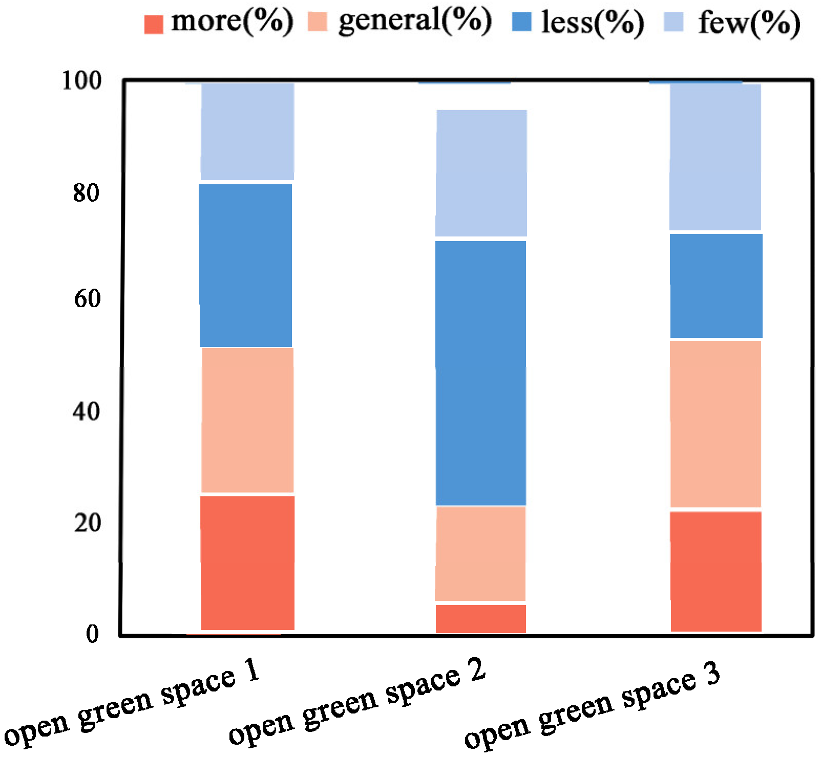
- Do you feel that the special weather (such as sandstorm, rainstorm, hail, extreme drought and extreme low temperature) in your place is frequent in the current season?○ many ○ more ○ general ○ less ○ few
- 8.
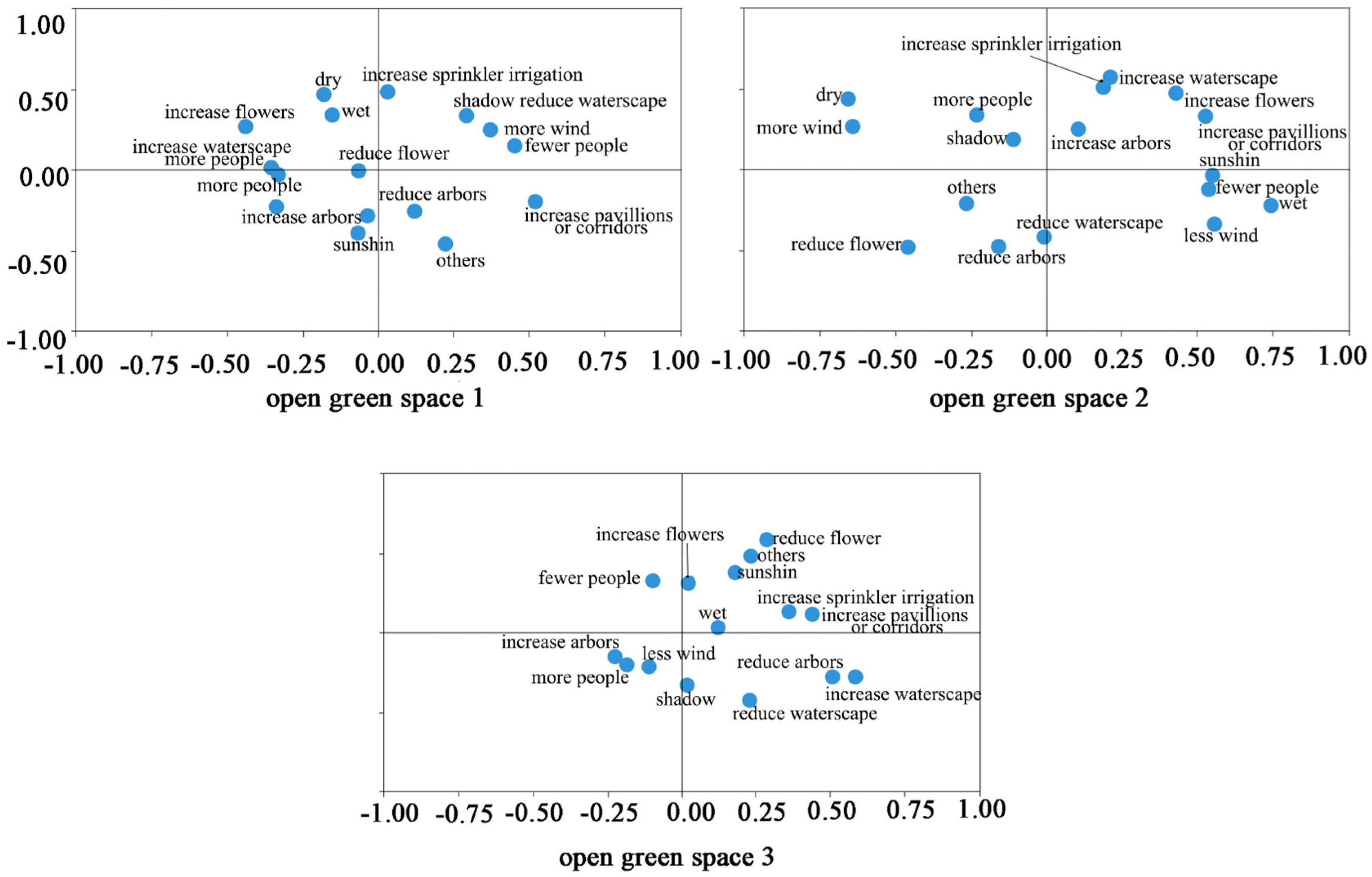
- Your preference for microclimate improvement (four groups, one from each group, four in total, and only four)□ more wind □ less wind □ wet □ dry □ sunshine □ shadow □ more people □ fewer people
- 9.
- Your preference for space improvement□ increase trees □ reduce trees □ increase flowers □ reduce flowers □ increase pavilions or corridors □ increase waterscape □ reduce waterscape □ increase sprinkler
Figure A1.
Open green space 1.
Figure A2.
Open green space 2.
Figure A3.
Open green space 3.
Appendix B
Table A1.
Meteorological variables in each measured space (Open green space 1).
Table A1.
Meteorological variables in each measured space (Open green space 1).
| Autumn (White Dew, 09,07) | Autumn (Cold Dew, 10,08) | Winter (Beginning of Winter, 11,07) | Winter (Winter Solstice, 12,07) | ||
|---|---|---|---|---|---|
| Va (m/s) | Juniperus formosana | 0.20 ± 0.006 Cd | 0.29 ± 0.006 Bbc | 0.34 ± 0.186 Bcd | 0.46 ± 0.009 Ae |
| Buxus megistophylla | 0.21 ± 0.006 Bd | 0.24 ± 0.23 ABc | 0.27 ± 0.067 ABd | 0.32 ± 0.009 Af | |
| Cedrus deodara | 0.54 ± 0.012 Ca | 0.60 ± 0.012 BCa | 0.64 ± 0.012 Ba | 0.77 ± 0.153 Aa | |
| Firmiana simplex | 0.39 ± 0.013 Bb | 0.58 ± 0.006 Aa | 0.60 ± 0.029 Aa | 0.68 ± 0.003 Ab | |
| Picea asperata | 0.18 ± 0.006 Cc | 0.55 ± 0.006 Ba | 0.67 ± 0.021 Aa | 0.73 ± 0.007 Aab | |
| Styphnolobium japonicum ‘Pendula’ | 0.14 ± 0.009 Dde | 0.29 ± 0.012 Cbc | 0.44 ± 0.021 Bb | 0.54 ± 0.003 Ad | |
| Juniperus chinensis | 0.18 ± 0.003 Ce | 0.27 ± 0.006 Bc | 0.31 ± 0.012 Bcd | 0.43 ± 0.012 Ae | |
| Betula platyphylla | 0.16 ± 0.012 Dde | 0.29 ± 0.006 Cbc | 0.40 ± 0.009 Bbc | 0.4 ± 0.007 Ae | |
| Pinus bungeana | 0.18 ± 0.003 Dde | 0.35 ± 0.006 Cb | 0.47 ± 0.006 Bb | 0.60 ± 0.003 Bc | |
| Prunus cerasifera f. atropurpurea | 0.24 ± 0.022 Ce | 0.23 ± 0.026 Ccde | 0.32 ± 0.015 Bcd | 0.46 ± 0.003 Ae | |
| Tg (°C) | Juniperus formosana | 6.68 ± 0.058 Bg | 9.47 ± 0.035 Ae | 5.68 ± 0.058 Cc | 3.03 ± 0.037 Df |
| Buxus megistophylla | 7.68 ± 0.115 Af | 6.97 ± 0.059 Bf | 6.68 ± 0.115 Bbc | 3.75 ± 0.100 Ce | |
| Cedrus deodara | 9.88 ± 0.115 ABe | 10.37 ± 0.344 Ade | 8.54 ± 0.240 Bab | 4.72 ± 0.039 Cbc | |
| Firmiana simplex | 11.62 ± 0.115 Ad | 11.57 ± 0.079 Bcd | 9.29 ± 0.240 Ca | 4.92 ± 0.039 Dab | |
| Picea asperata | 14.82 ± 0.231 ABab | 15.56 ± 0.510 Aa | 10.59 ± 0.489 Ba | 5.16 ± 0.023 Ca | |
| Styphnolobium japonicum ‘Pendula’ | 15.68 ± 0.058 Aa | 15.50 ± 0.137 Aa | 9.67 ± 0.947 Ba | 4.55 ± 0.029 Cc | |
| Juniperus chinensis | 13.51 ± 0.058 Ac | 13.02 ± 0.203 Ab | 10.18 ± 0.285 Ba | 4.14 ± 0.031 Cdc | |
| Betula platyphylla | 14.09 ± 0.379 Ab | 12.15 ± 0.082 Abc | 9.14 ± 0.603 Bab | 3.55 ± 0.068 Ce | |
| Pinus bungeana | 11.25 ± 0.058 Ad | 11.10 ± 0.029 Acd | 8.57 ± 0.368 Bab | 4.07 ± 0.033 Cd | |
| Prunus cerasifera f. atropurpurea | 11.60 ± 0.173 Ad | 11.86 ± 0.449 Ac | 10.08 ± 0.139 Ba | 3.82 ± 0.093 Cde | |
| Ta (°C) | Juniperus formosana | 5.29 ± 0.035 Ah | 4.51 ± 0.067 Bf | 3.15 ± 0.29 Cde | 1.00 ± 0.115 Dc |
| Buxus megistophylla | 6.41 ± 0.234 Ag | 5.93 ± 0.077 Af | 3.44 ± 0.04 Bde | 1.6 ± 0.305 Cbc | |
| Cedrus deodara | 9.69 ± 0.058 Af | 9.44 ± 0.172 Ad | 4.79 ± 0.105 Bbc | 2.23 ± 0.120 Cab | |
| Firmiana simplex | 13.78 ± 0.058 Ac | 13.22 ± 0.563 Ab | 5.89 ± 0.064 Ba | 2.45 ± 0.029 Ca | |
| Picea asperata | 14.73 ± 0.115 Ab | 15.09 ± 0.266 Aa | 5.48 ± 0.290 Bab | 2.53 ± 0.176 Ca | |
| Styphnolobium japonicum ‘Pendula’ | 17.78 ± 0.115 Aa | 16.35 ± 0.448 Aa | 5.11 ± 0.437 Babc | 2.15 ± 0.755 Cab | |
| Juniperus chinensis | 14.08 ± 0.310 Abc | 13.17 ± 0.138 Ab | 4.81 ± 0.064 Bbc | 1.93 ± 0.064 aCb | |
| Betula platyphylla | 12.65 ± 0.006 Ad | 11.53 ± 0.120 Bc | 4.33 ± 0.088 Ccd | 1.83 ± 0.035 Dab | |
| Pinus bungeana | 10.72 ± 0.115 Ae | 10.22 ± 0.173 Acd | 4.19 ± 0.034 Bcd | 1.45 ± 0.074 Cbc | |
| Prunus cerasifera f. atropurpurea | 11.23 ± 0.115 Ae | 10.74 ± 0.278 Acd | 4.17 ± 0.037 Bcd | 1.86 ± 0.094 Cbc | |
| RH (%) | Juniperus formosana | 60.84 ± 0.462 Aa | 59.28 ± 0.577 Aa | 54.85 ± 0.356 Ba | 47.33 ± 0.362 Cab |
| Buxus megistophylla | 54.28 ± 1.707 ABc | 57.35 ± 1.468 Aa | 48.35 ± 0.233 BCc | 43.57 ± 0.513 Cc | |
| Cedrus deodara | 49.49 ± 0.450 Ad | 45.49 ± 0.577 ABb | 42.49 ± 1.154 Bde | 35.57 ± 0.384 Ce | |
| Firmiana simplex | 37.06 ± 0.766 Af | 36.3 ± 0.058 Ac | 34.07 ± 0.521 ABf | 31.83 ± 0.273 Bf | |
| Picea asperata | 35.81 ± 0.181 Af | 37.47 ± 0.231 Ac | 32.90 ± 0.385 Bf | 31.08 ± 0.586 Bf | |
| Styphnolobium japonicum ‘Pendula’ | 38.53 ± 0.312 Af | 33.21 ± 0.008 Bc | 29.88 ± 0.252 Cg | 27.96 ± 0.281 Dg | |
| Juniperus chinensis | 45.38 ± 0.347 Ae | 45.03 ± 0.017 Ab | 40.36 ± 0.384 Be | 35.99 ± 0.564 Ce | |
| Betula platyphylla | 53.28 ± 0.398 Acd | 50.53 ± 0.058 Ab | 44.36 ± 0.285 Bd | 39.15 ± 0.596 Cd | |
| Pinus bungeana | 69.94 ± 0.436 Aa | 62.57 ± 0.231 Ba | 51.19 ± 0.748 Cbc | 45.70 ± 0.439 Dbc | |
| Prunus cerasifera f. atropurpurea | 59.57 ± 0.637 Ab | 62.31 ± 3.535 Ab | 53.76 ± 0.286 Aab | 49.76 ± 0.694 Aa | |
| Vv (cmm) | Juniperus formosana | 13.47 ± 0.049 Ce | 21.74 ± 0.577 Bc | 26.13 ± 0.196 Ac | 28.04 ± 0.294 Ade |
| Buxus megistophylla | 16.45 ± 0.654 Bd | 17.83 ± 0.058 Be | 19.16 ± 0.338 ABd | 20.66 ± 0.172 Af | |
| Cedrus deodara | 39.93 ± 0.126 Ca | 42.11 ± 0.577 BCa | 44.11 ± 0.577 Ba | 47.72 ± 0.434 Aa | |
| Firmiana simplex | 26.66 ± 0.234 Cb | 40.93 ± 0.231 Ba | 42.11 ± 0.485 ABa | 44.42 ± 0.354 Ab | |
| Picea asperata | 21.25 ± 0.598 Cc | 40.46 ± 0.231 Ba | 43.41 ± 0.516 ABa | 45.4 ± 0.468 Aab | |
| Styphnolobium japonicum ‘Pendula’ | 14.32 ± 0.244 Ce | 21.16 ± 0.577 Bcd | 25.07 ± 0.093 Ac | 27.59 ± 0.581 Ade | |
| Juniperus chinensis | 10.28 ± 0.124 Cfe | 18.89 ± 0.346 Bde | 24.22 ± 0.647 Ac | 26.02 ± 0.690 Ae | |
| Betula platyphylla | 10.43 ± 0.86 Cf | 20.67 ± 0.577 Bcd | 26.67 ± 0.577 Ac | 30.07 ± 0.636 Ac | |
| Pinus bungeana | 11.00 ± 0.299 Df | 24.97 ± 0.520 Cb | 29.30 ± 0.383 Bb | 33.25 ± 0.653 Ad | |
| Prunus cerasifera f. atropurpurea | 13.86 ± 0.200 De | 16.26 ± 0.115 Bf | 10.14 ± 0.130 Bd | 25.29 ± 0.420 Ae |
Notes: Values are performed as mean values ± standard errors. The different normal letters in the same column indicate significant differences among treatments at the 0.001 level, while the different capital letters in the same row indicate significant differences among stages at the 0.001 level. The same is shown below.
Table A2.
Meteorological variables in each measured space (Open green space 2).
Table A2.
Meteorological variables in each measured space (Open green space 2).
| Autumn (White Dew, 09,07) | Autumn (Cold Dew, 10,08) | Winter (Beginning of Winter, 11,07) | Winter (Winter Solstice, 12,07) | ||
|---|---|---|---|---|---|
| Va (m/s) | Berberis thunbergii ‘Atropurpurea’ | 0.44 ± 0.009 Cd | 0.55 ± 0.009 Be | 0.60 ± 0.009 Be | 0.78 ± 0.012 Ae |
| Ligustrum lucidum | 0.25 ± 0.003 Df | 0.31 ± 0.003 Cg | 0.43 ± 0.003 Bf | 0.53 ± 0.009 Ag | |
| Cornus alba | 0.29 ± 0.003 Df | 0.36 ± 0.003 Cfg | 0.47 ± 0.003 Bf | 0.67 ± 0.009 Af | |
| Syringa oblata | 0.92 ± 0.012 Ca | 1.15 ± 0.070 BCa | 1.31 ± 0.006 Ba | 1.58 ± 0.009 Aa | |
| Forsythia suspense | 0.50 ± 0.009 Dc | 0.760 ± 0.006 Cd | 0.87 ± 0.003 Bd | 0.94 ± 0.009 Ad | |
| Lonicera maackii | 0.38 ± 0.012 De | 0.80 ± 0.012 Ccd | 0.92 ± 0.009 Bc | 1.20 ± 0.026 Ac | |
| Prunus triloba | 0.40 ± 0.009 Dde | 0.96 ± 0.034 Cb | 1.21 ± 0.009 Bb | 1.55 ± 0.029 Aa | |
| Lonicera japonica | 0.38 ± 0.009 Ce | 0.50 ± 0.009 Bef | 0.58 ± 0.019 ABe | 0.6 ± 0.003 Ag | |
| Rosa xanthina | 0.27 ± 0.009 Df | 0.34 ± 0.006 Cg | 0.36 ± 0.011 Bg | 0.38 ± 0.012 Ah | |
| Buxus sinica var. parvifolia | 0.60 ± 0.012 Db | 0.92 ± 0.012 Cbc | 1.24 ± 0.003 Bb | 1.44 ± 0.027 Ab | |
| Tg (°C) | Berberis thunbergii ‘Atropurpurea’ | 11.08 ± 0.319 Ad | 9.74 ± 0.142 Bf | 7.93 ± 0.045 Ce | 4.23 ± 0.105 Df |
| Ligustrum lucidum | 14.20 ± 0.220 Ac | 12.56 ± 0.280 Be | 10.31 ± 0.048 Cbc | 7.28 ± 0.085 Dd | |
| Cornus alba | 14.75 ± 0.313 Abc | 13.17 ± 0.263 ABde | 11.70 ± 0.2482 Bab | 8.19 ± 0.195 Cbcd | |
| Syringa oblata | 15.81 ± 0.217 Aabc | 14.72 ± 0.172 Aabc | 12.37 ± 0.186 Ba | 9.84 ± 0.199 Ca | |
| Forsythia suspense | 14.01 ± 0.194 Ac | 13.28 ± 0.283 Ade | 11.48 ± 0.260 Bab | 8.91 ± 0.067 Cb | |
| Lonicera maackii | 15.50 ± 0.430 Aabc | 13.80 ± 0.104 Acde | 10.61 ± 0.207 Bbc | 8.34 ± 0.175 Cbc | |
| Prunus triloba | 16.78 ± 0.296 Aab | 15.14 ± 0.227 Aabc | 9.97 ± 0.289 Bcd | 7.92 ± 0.192 Ccd | |
| Lonicera japonica | 16.15 ± 0.090 Aa | 15.96 ± 0.166 Aa | 11.25 ± 0.132 Bab | 7.38 ± 0.204 Ccd | |
| Rosa xanthina | 14.11 ± 0.379 Ac | 14.17 ± 0.361 Abc | 8.93 ± 0.185 Bde | 6.09 ± 0.152 Ce | |
| Buxus sinica var. parvifolia | 16.27 ± 0.506 Aab | 15.37 ± 0.179 Aab | 12.41 ± 0.226 Ba | 8.18 ± 0.193 Cbcd | |
| Ta (°C) | Berberis thunbergii ‘Atropurpurea’ | 9.32 ± 0.291 Af | 8.52 ± 0.271 fAB | 7.10 ± 0.381 Be | 2.64 ± 0.225 Ce |
| Ligustrum lucidum | 12.81 ± 0.208 Ae | 11.15 ± 0.173 Be | 9.41 ± 0.031 Cbc | 4.4 ± 0.144 Dcd | |
| Cornus alba | 13.16 ± 0.148 Ae | 12.24 ± 0.242 Ade | 10.16 ± 0.212 Bab | 5.14 ± 0.081 Cb | |
| Syringa oblata | 14.28 ± 0.147 Ade | 11.96 ± 0.205 Bde | 11.07 ± 0.204 Ba | 6.43 ± 0.278 Ca | |
| Forsythia suspense | 14.72 ± 0.280 Acd | 13.77 ± 0.283 Abc | 10.03 ± 0.107 Babc | 5.65 ± 0.124 Cab | |
| Lonicera maackii | 13.94 ± 0.327 Ade | 12.57 ± 0.259 Acd | 8.16 ± 0.114 Bd | 4.06 ± 0.035 Ccd | |
| Prunus triloba | 17.92 ± 0.290 Aa | 15.34 ± 0.189 Ba | 9.02 ± 0.194 Ccd | 3.20 ± 0.190 De | |
| Lonicera japonica | 16.83 ± 0.334 Aab | 15.36 ± 0.079 Ba | 9.87 ± 0.046 Cbc | 4.66 ± 0.087 Dbcd | |
| Rosa xanthina | 13.32 ± 0.132 Ade | 12.47 ± 0.241 Ad | 6.78 ± 0.156 Be | 3.07 ± 0.060 Ce | |
| Buxus sinica var. parvifolia | 15.83 ± 0.311 Abc | 14.2 ± 0.248 Bab | 8.28 ± 0.142 Cd | 4.29 ± 0.032 Dcd | |
| RH (%) | Berberis thunbergii ‘Atropurpurea’ | 38.58 ± 0.362 Ad | 37.11 ± 0.497 Ad | 33.91 ± 0.233 Bcd | 30.27 ± 0.402 Ce |
| Ligustrum lucidum | 54.69 ± 0.347 Ab | 50.68 ± 0.320 Bb | 47.79 ± 0.406 Cb | 45.38 ± 0.504 Cb | |
| Cornus alba | 53.87 ± 0.473 Abc | 49.35 ± 0.621 Bbc | 47.17 ± 0.315 BCb | 45.52 ± 0.457 Cb | |
| Syringa oblata | 80.18 ± 0.434 Aa | 76.52 ± 0.305 Ba | 71.00 ± 0.197 Ca | 62.73 ± 0.095 Da | |
| Forsythia suspense | 37.97 ± 0.266 Ade | 35.09 ± 0.199 Bde | 31.91 ± 0.282 Cef | 29.93 ± 0.131 De | |
| Lonicera maackii | 38.74 ± 0.311 Ad | 36.70 ± 0.345 Bde | 34.91 ± 0.278 BCc | 33.04 ± 0.038 Cd | |
| Prunus triloba | 33.58 ± 0.600 Af | 29.76 ± 0.187 Bf | 31.21 ± 0.116 BCf | 28.03 ± 0.148 Cf | |
| Lonicera japonica | 38.23 ± 0.257 Ade | 35.65 ± 0.618 ABde | 34.27 ± 0.168 Bcd | 30.72 ± 0.458 Ce | |
| Rosa xanthina | 51.34 ± 0.587 Ac | 47.75 ± 0.273 Bc | 47.99 ± 0.245 Bb | 42.76 ± 0.123 Cc | |
| Buxus sinica var. parvifolia | 35.97 ± 0.407 Ae | 34.63 ± 0.486 ABe | 32.82 ± 0.289 Bde | 28.18 ± 0.162 Cf | |
| Vv (cmm) | Berberis thunbergii ‘Atropurpurea’ | 52.63 ± 0.315 Da | 57.65 ± 0.415 Cd | 61.15 ± 0.436 Bd | 67.22 ± 0.503 Ac |
| Ligustrum lucidum | 32.82 ± 0.356 Dde | 35.73 ± 0.499 Cf | 38.78 ± 0.411 Bg | 49.07 ± 0.249 Ae | |
| Cornus alba | 34.11 ± 0.312 Dd | 39.23 ± 0.422 Cf | 42.81 ± 0.217 Bf | 53.75 ± 0.289 Ad | |
| Syringa oblata | 22.37 ± 0.606 Dg | 30.43 ± 0.396 Ch | 38.60 ± 0.234 Bg | 45.49 ± 0.557 Af | |
| Forsythia suspense | 39.12 ± 0.778 Dc | 55.43 ± 0.674 Cd | 62.12 ± 0.334 Bd | 68.08 ± 0.394 Ac | |
| Lonicera maackii | 27.50 ± 0.471 Df | 61.50 ± 0.712 Cb | 64.85 ± 0.331 Bc | 72.16 ± 0.105 Ab | |
| Prunus triloba | 26.82 ± 0.301 Cf | 70.88 ± 1.075 Ba | 75.01 ± 0.133 ABa | 77.46 ± 0.291 Aa | |
| Lonicera japonica | 30.36 ± 0.700 De | 42.88 ± 0.418 Ce | 46.11 ± 0.105 Be | 50.56 ± 0.296 Ae | |
| Rosa xanthina | 20.98 ± 0.267 Db | 24.41 ± 0.655 Ci | 27.46 ± 0.275 Bh | 34.05 ± 0.226 Ag | |
| Buxus sinica var. parvifolia | 42.07 ± 0.410 Dg | 66.58 ± 0.754 Cb | 71.70 ± 0.158 Bbd | 75.97 ± 0.163 Aa |
Notes: Values are performed as mean values ± standard errors. The different normal letters in the same column indicate significant differences among treatments at the 0.001 level, while the different capital letters in the same row indicate significant differences among stages at the 0.001 level.
Table A3.
Meteorological variables in each measured space (Open green space 3).
Table A3.
Meteorological variables in each measured space (Open green space 3).
| Autumn (White Dew, 09,07) | Autumn (Cold Dew, 10,08) | Winter (Beginning of Winter, 11,07) | Winter (Winter Solstice, 11,07) | ||||||||||
|---|---|---|---|---|---|---|---|---|---|---|---|---|---|
| OGS1 | OGS2 | OGS3 | OGS1 | OGS2 | OGS3 | OGS1 | OGS2 | OGS3 | OGS1 | OGS2 | OGS3 | ||
| Va (m/s) | H | 0.45 ± 0.003 d | 0.44 ± 0.003 d | 0.41 ± 0.009 d | 0.61 ± 0.009 c | 0.58 ± 0.006 c | 0.51 ± 0.009 c | 0.76 ± 0.006 b | 0.68 ± 0.012 b | 0.60 ± 0.138 b | 0.82 ± 0.009 a | 0.78 ± 0.003 a | 0.76 ± 0.012 a |
| SH | 0.43 ± 0.010 d | 0.41 ± 0.06 d | 0.35 ± 0.003 d | 0.59 ± 0.153 c | 0.56 ± 0.06 c | 0.50 ± 0.009 c | 0.71 ± 0.011 b | 0.69 ± 0.06 b | 0.66 ± 0.003 b | 0.77 ± 0.010 a | 0.74 ± 0.0.09 a | 0.71 ± 0.007 a | |
| AH | 0.40 ± 0.003 d | 0.37 ± 0.006 d | 0.31 ± 0.009 d | 0.50 ± 0.009 c | 0.47 ± 0.010 c | 0.45 ± 0.006 c | 0.62 ± 0.011 b | 0.61 ± 0.019 b | 0.58 ± 0.009 b | 0.70 ± 0.009 a | 0.68 ± 0.006 a | 0.66 ± 0.006 a | |
| ASH | 0.36 ± 0.003 d | 0.34 ± 0.003 d | 0.23 ± 0.007 c | 0.41 ± 0.003 c | 0.38 ± 0.006 c | 0.39 ± 0.006 b | 0.54 ± 0.007 b | 0.53 ± 0.003 b | 0.53 ± 0.009 a | 0.66 ± 0.003 a | 0.57 ± 0.003 a | 0.57 ± 0.007 a | |
| Tg (°C) | H | 9.24 ± 0.118 a | 8.39 ± 0.203 a | 8.08 ± 0.040 a | 7.43 ± 0.082 b | 7.36 ± 0.197 a | 7.23 ± 0.145 b | 5.37 ± 0.116 b | 5.20 ± 0.145 c | 5.13 ± 0.064 c | 4.03 ± 0.088 d | 4.03 ± 0.058 c | 3.70 ± 0.058 d |
| SH | 11.40 ± 0.529 a | 10.50 ± 0.265 a | 10.13 ± 0.188 a | 9.83 ± 0.764 a | 8.77 ± 0.145 b | 8.45 ± 0.232 b | 7.43 ± 0.404 b | 7.43 ± 0.404 b | 7.15 ± 0.736 c | 5.73 ± 0.246 c | 4.93 ± 0.115 c | 4.80 ± 0.058 d | |
| AH | 13.97 ± 0.058 a | 13.33 ± 0.203 a | 12.40 ± 0.36 a | 12.40 ± 0.208 a | 11.43 ± 0.379 b | 9.69 ± 0.64 b | 8.97 ± 0.162 c | 8.57 ± 0.296 b | 8.15 ± 0.101 c | 7.41 ± 0.059 c | 6.35 ± 0.174 c | 6.08 ± 0.231 d | |
| ASH | 11.43 ± 0.047 a | 11.28 ± 0.017 d | 11.20 ± 0.103 a | 10.31 ± 0.112 b | 10.17 ± 0.089 a | 10.07 ± 0.033 c | 9.54 ± 0.123 b | 8.35 ± 0.029 b | 8.28 ± 0.041 b | 8.17 ± 0.112 c | 5.11 ± 0.070 a | 4.60 ± 0.750 c | |
| Ta (°C) | H | 7.45 ± 0.247 a | 7.32 ± 0.072 a | 7.06 ± 0.067 a | 5.94 ± 0.068 b | 5.74 ± 0.029 b | 5.11 ± 0.067 b | 3.35 ± 0.084 c | 2.15 ± 0.077 c | 2.03 ± 0.033 c | 2.06 ± 0.173 d | 1.76 ± 0.031 c | 1.55 ± 0.029 d |
| SH | 8.4 ± 0.100 a | 8.38 ± 0.044 a | 8.10 ± 0.100 a | 7.03 ± 0.033 b | 6.45 ± 0.234 b | 5.93 ± 0.120 b | 4.39 ± 0.194 c | 4.03 ± 0.088 c | 3.97 ± 0.148 c | 3.18 ± 0.356 c | 2.10 ± 0.058 d | 1.90 ± 0.058 d | |
| AH | 12.10 ± 0.208 a | 11.60 ± 0.400 a | 10.50 ± 0.289 a | 9.73 ± 0.371 b | 9.19 ± 0.335 b | 7.60 ± 0.306 b | 5.23 ± 0.186 c | 5.07 ± 0.067 c | 4.90 ± 0.100 c | 4.47 ± 0.72 c | 4.17 ± 0.120 c | 4.07 ± 0.115 c | |
| ASH | 11.60 ± 0.400 a | 9.92 ± 0.043 a | 8.33 ± 0.067 a | 9.15 ± 0.074 b | 8.50 ± 0.055 a | 8.48 ± 0.018 a | 6.82 ± 0.064 b | 5.78 ± 0.056 b | 4.58 ± 0.100 c | 5.19 ± 0.241 c | 3.18 ± 0.020 d | 3.15 ± 0.046 c | |
| RH (%) | H | 36.68 ± 0.387 a | 35.44 ± 0.281 a | 34.85 ± 0.147 a | 34.23 ± 0.448 ab | 33.60 ± 0.359 a | 32.71 ± 0.359 a | 31.27 ± 0.410 b | 30.82 ± 0.431 b | 29.47 ± 0.309 b | 25.19 ± 0.478 c | 24.52 ± 0.289 c | 23.27 ± 0.601 c |
| SH | 48.56 ± 0.294 a | 48.27 ± 0.267 a | 38.7 ± 0.153 a | 44.90 ± 0.493 b | 42.47 ± 0.291 b | 37.04 ± 0.166 ab | 41.15 ± 0.597 c | 39.80 ± 0.115 c | 34.71 ± 0.389 b | 36.82 ± 0.429 d | 35.90 ± 0.493 d | 29.04 ± 0.615 c | |
| AH | 52.60 ± 0.529 a | 55.27 ± 0.819 a | 41.7 ± 0.351 a | 49.30 ± 0.351 b | 47.60 ± 0.529 b | 39.27 ± 0.636 ab | 44.97 ± 0.35 bc | 42.85 ± 0.790 c | 37.17 ± 0.119 bc | 40.33 ± 0.882 c | 37.5 ± 0.500 d | 35.09 ± 0.327 c | |
| ASH | 49.27 ± 0.357 a | 49.21 ± 0.116 a | 38.82 ± 0.133 a | 47.4 ± 0.200 b | 45.15 ± 0.076 b | 38.26 ± 0.173 b | 42.59 ± 0.049 c | 41.69 ± 0.164 c | 36.76 ± 0.148 b | 37.54 ± 0.356 d | 37.21 ± 0.107 d | 35.00 ± 0.234 c | |
| Vv (cmm) | H | 41.90 ± 0.466 d | 41.00 ± 0.577 d | 40.93 ± 0.468 d | 52.16 ± 0.443 c | 51.05 ± 0.621 c | 48.41 ± 0.747 c | 67.74 ± 0.378 b | 66.45 ± 0.294 b | 57.42 ± 0.550 b | 73.53 ± 0.290 a | 70.67 ± 0.333 a | 67.27 ± 1.124 a |
| SH | 40.03 ± 0.260 d | 39.73 ± 0.187 d | 39.00 ± 0.500 d | 49.47 ± 0.502 c | 48.90 ± 0.587 c | 47.59 ± 0.549 c | 64.74 ± 0.378 b | 64.19 ± 0.424 b | 56.49 ± 0.866 b | 70.29 ± 0.618 a | 69.29 ± 0.633 a | 61.34 ± 0.393 a | |
| AH | 38.93 ± 0.515 d | 37.50 ± 0.500 d | 34.45 ± 0.292 c | 50.00 ± 1.155 c | 49.00 ± 1.000 c | 46.17 ± 0.647 b | 60.33 ± 1.155 b | 59.67 ± 1.528 b | 55.81 ± 0.226 a | 68.33 ± 0.333 a | 66.33 ± 0.577 a | 57.62 ± 0.314 a | |
| ASH | 36.60 ± 0.150 d | 34.96 ± 0.031 d | 29.18 ± 0.157 d | 54.78 ± 0.048 b | 46.21 ± 0.107 c | 44.56 ± 0.300 c | 57.14 ± 0.305 b | 54.78 ± 0.048 b | 46.45 ± 0.121 b | 74.78 ± 0.264 a | 66.14 ± 0.071 a | 56.75 ± 0.411 a | |
OGS: Open green space. (a, b, c, d are difference significance analysis, a is significant difference, and so on).
References
- Kovats, R.S.; Hajat, S. Heat stress and public health: A critical review. Annu. Rev. Public Health 2008, 29, 41–55. [Google Scholar] [CrossRef]
- Chen, H.; Ooka, R.; Kato, S. Study on optimum arrangement of pilotis for design of pleasant outdoor wind environment using CFD simulation and Genetic Algorithms (GA). In Proceedings of the Sixth Asia-Pacific Conference on Wind Engineering (APCWE-VI), Seoul, Republic of Korea; 2005; pp. 1–11. [Google Scholar]
- Zellweger, F.; De Frenne, P.; Lenoir, J.; Rocchini, D.; Coomes, D. Advances in Microclimate Ecology Arising from Remote Sensing. Trends Ecol. Evol. 2019, 34, 327–341. [Google Scholar] [CrossRef] [PubMed]
- Li, X.X.; Norford, L.K. Evaluation of cool roof and vegetations in mitigating urban heat island in a tropical city, Singapore. Urban Clim. 2016, 16, 59–74. [Google Scholar] [CrossRef]
- Mushtaha, E.; Shareef, S.; Alsyouf, I.; Mori, T.; Kayed, A.; Abdelrahim, M.; Albannay, S. A study of the impact of major Urban Heat Island factors in a hot climate courtyard: The case of the University of Sharjah, UAE. Sustain. Cities Soc. 2021, 69, 15. [Google Scholar] [CrossRef]
- Zhang, T.; Su, M.; Hong, B.; Wang, C.; Li, K. Interaction of emotional regulation and outdoor thermal perception: A pilot study in a cold region of China. Build. Environ. 2021, 198, 107870. [Google Scholar] [CrossRef]
- Salmond, J.A.; Tadaki, M.; Vardoulakis, S.; Arbuthnott, K.; Coutts, A.; Demuzere, M.; Dirks, K.N.; Heaviside, C.; Lim, S.; Maintyre, H.; et al. Health and climate related ecosystem services provided by street trees in the urban environment. Environ. Health 2016, 15 (Suppl. 1), 36. [Google Scholar] [CrossRef]
- Dimoudi, A.; Nikolopoulou, M. Vegetation in the urban environment: Microclimatic analysis and benefits. Energy Build. 2003, 35, 69–76. [Google Scholar] [CrossRef]
- Elwy, I.; Ibrahim, Y.; Fahmy, M.; Mahdy, M. Outdoor microclimatic validation for hybrid simulation workflow in hot arid climates against ENVI-met and field measurements. Energy Procedia 2018, 153, 29–34. [Google Scholar] [CrossRef]
- Bajšanski, I.V.; Milošević, D.D.; Savić, S.M. Evaluation and improvement of outdoor thermal comfort in urban areas on extreme temperature days: Applications of automatic algorithms. Build. Environ. 2015, 94, 632–643. [Google Scholar] [CrossRef]
- Zhang, T.; Hong, B.; Su, X.; Li, Y.; Song, L. Effects of tree seasonal characteristics on thermal-visual perception and thermal comfort. Build. Environ. 2022, 212, 108793. [Google Scholar] [CrossRef]
- Hami, A.; Abdi, B.; Zarehaghi, D.; Maulan, S.B. Assessing the thermal comfort effects of green spaces: A systematic review of methods, parameters, and plants’ attributes. Sustain. Cities Soc. 2019, 49, 11. [Google Scholar] [CrossRef]
- Ma, X.; Tian, Y.; Du, M.; Hong, B.; Lin, B. How to design comfortable open spaces for the elderly? Implications of their thermal perceptions in an urban park. Sci. Total Environ. 2021, 768, 144985. [Google Scholar] [CrossRef]
- Yuan, T.; Hong, B.; Qu, H.; Liu, A.; Zheng, Y. Outdoor thermal comfort in urban and rural open spaces: A comparative study in China’s cold region. Urban Clim. 2023, 49, 101501. [Google Scholar] [CrossRef]
- Natanian, J.; Kastner, P.; Dogan, T.; Auer, T. From energy performative to livable Mediterranean cities: An annual outdoor thermal comfort and energy balance cross-climatic typological study. Energy Build. 2020, 224, 18. [Google Scholar] [CrossRef]
- Bröde, P.; Jendritzky, G.; Fiala, D.; Havenith, G. The Universal Thermal Climate Index UTCI in operational use. In Proceedings of the Adapting to Change: New Thinking on Comfort, Windsor, UK, 9–11 April 2010. [Google Scholar]
- Fang, Y.; Cho, S. Design optimization of building geometry and fenestration for daylighting and energy performance. Sol. Energy 2019, 191, 7–18. [Google Scholar] [CrossRef]
- Ibrahim, Y.; Kershaw, T.; Shepherd, P.; Elwy, I. A parametric optimisation study of urban geometry design to assess outdoor thermal comfort. Sustain. Cities Soc. 2021, 75, 103352. [Google Scholar] [CrossRef]
- Zhang, Q.; Li, X.; Wang, Y. Analysis of climatic characteristics and trends in Lanzhou City during 1981–2016. Environ. Sci. Pollut. Res. 2020, 27, 32965–32977. [Google Scholar]
- Bueno, B.; Norford, L.; Hidalgo, J.; Pigeon, G. The urban weather generator. J. Build. Perform. Simul. 2013, 6, 269–281. [Google Scholar] [CrossRef]
- Bueno, B.; Roth, M.; Norford, L.; Li, R. Computationally efficient prediction of canopy level urban air temperature at the neighbourhood scale. Urban Clim. 2014, 9, 35–53. [Google Scholar] [CrossRef]
- Xu, Y.; Liu, X.; Hu, Y.; Deng, Y.; Li, M. Influence of different tree species on wind environment in urban green spaces: A case study in Guangzhou, China. Urban For. Urban Green. 2019, 38, 302–310. [Google Scholar]
- Shooshtarian, S.; Ridley, I. The effect of physical and psychological environments on the users thermal perceptions of educational urban precincts. Build. Environ. 2017, 115, 182–198. [Google Scholar] [CrossRef]
- Galindo, T.; Hermida, M.A. Effects of thermophysiological and non-thermal factors on outdoor thermal perceptions: The Tomebamba Riverbanks case. Build. Environ. 2018, 138, 235–249. [Google Scholar] [CrossRef]
- Yahia, M.W.; Johansson, E.; Thorsson, S.; Lindberg, F.; Rasmussen, M.I. Effect of urban design on microclimate and thermal comfort outdoors in warm-humid Dar es Salaam, Tanzania. Int. J. Biometeorol. 2018, 62, 373–385. [Google Scholar] [CrossRef] [PubMed]
- Sun, T.; Li, X.; Cheng, W.; Zhou, Y.; Wang, M.; Liu, W. Quantifying the impacts of meteorological factors on the urban heat island effect using a spatially explicit network model. Sci. Total Environ. 2021, 753, 141947. [Google Scholar]
- Yang, Z.; Hanna, E.; Callaghan, T.V.; Jonasson, C. How can meteorological observations and microclimate simulations improve understanding of 1913–2010 climate change around Abisko, Swedish Lapland? Meteorol. Appl. 2012, 19, 454–463. [Google Scholar] [CrossRef]
- Piselli, C.; Castaldo, V.L.; Pigliautile, I.; Pisello, A.L.; Cotana, F. Outdoor comfort conditions in urban areas: On citizens’ perspective about microclimate mitigation of urban transit areas. Sustain. Cities Soc. 2018, 39, 16–36. [Google Scholar] [CrossRef]
- Burstrom, L.; Bjor, B.; Nilsson, T.; Pettersson, H.; Rodin, I.; Wahlstrom, J. Thermal perception thresholds among workers in a cold climate. Int. Arch. Occup. Environ. Health 2017, 90, 645–652. [Google Scholar] [CrossRef]
- Jowkar, M.; Rijal, H.B.; Montazami, A.; Brusey, J.; Temeljotov-Salaj, A. The influence of acclimatization, age and gender-related differences on thermal perception in university buildings: Case studies in Scotland and England. Build. Environ. 2020, 179, 106933. [Google Scholar] [CrossRef]
- Chang, J.; Du, M.; Hong, B.; Qu, H.; Chen, H. Effects of thermal-olfactory interactions on emotional changes in urban outdoor environments. Build. Environ. 2023, 232, 110049. [Google Scholar] [CrossRef]
- Othman, N.E.; Zaki, S.A.; Rijal, H.B.; Ahmad, N.H.; Razak, A.A. Field study of pedestrians' comfort temperatures under outdoor and semi-outdoor conditions in Malaysian university campuses. Int. J. Biometeorol. 2021, 65, 453–477. [Google Scholar] [CrossRef]
- Saroglou, T.; Itzhak-Ben-Shalom, H.; Meir, I.A. Pedestrian thermal perception: Studies around two high-rise buildings in the Mediterranean climate. Build. Res. Inf. 2021, 50, 171–191. [Google Scholar] [CrossRef]
- Peng, Y.; Peng, Z.; Feng, T.; Zhong, C.; Wang, W. Assessing Comfort in Urban Public Spaces: A Structural Equation Model Involving Environmental Attitude and Perception. Int. J. Environ. Res. Public Health 2021, 18, 17. [Google Scholar] [CrossRef] [PubMed]
- Ma, X.; Song, L.; Hong, B.; Li, Y.; Li, Y. Relationships between EEG and thermal comfort of elderly adults in outdoor open spaces. Build. Environ. 2023, 235, 110212. [Google Scholar] [CrossRef]
- Li, Y.; Hong, B.; Wang, Y.; Bai, H.; Chen, H. Assessing heat stress relief measures to enhance outdoor thermal comfort: A field study in China’s cold region. Sustain. Cities Soc. 2022, 80, 103813. [Google Scholar] [CrossRef]
- Crawley, D.B.; Lawrie, L.K.; Winkelmann, F.C.; Buhl, W.F.; Huang, Y.J.; Pedersen, C.O.; Strand, R.K.; Liesen, R.J.; Fisher, D.E.; Witter, M.J.; et al. EnergyPlus: Creating a new-generation building energy simulation program. Energy Build. 2001, 33, 319–331. [Google Scholar] [CrossRef]
- Evola, G.; Marletta, L.; Cimino, D. Weather data morphing to improve building energy modeling in an urban context. Math. Model. Eng. Probl. 2018, 5, 211–216. [Google Scholar] [CrossRef]
Disclaimer/Publisher’s Note: The statements, opinions and data contained in all publications are solely those of the individual author(s) and contributor(s) and not of MDPI and/or the editor(s). MDPI and/or the editor(s) disclaim responsibility for any injury to people or property resulting from any ideas, methods, instructions or products referred to in the content. |
© 2023 by the authors. Licensee MDPI, Basel, Switzerland. This article is an open access article distributed under the terms and conditions of the Creative Commons Attribution (CC BY) license (https://creativecommons.org/licenses/by/4.0/).