Abstract
The radiant ceiling cooling system is widely adopted in modern office buildings as it improves cooling source efficiency and reduces fossil fuel usage and carbon dioxide emissions by utilizing low-grade natural energy. However, the nonlinear behavior and significant inertia of the radiant ceiling cooling system pose challenges for control systems. With advancements in computer technology and artificial intelligence, the deep reinforcement learning (DRL) method shows promise in the operation and control of radiant cooling systems with large inertia. This paper compares the DRL control method with traditional control methods for radiant ceiling cooling systems in two typical office rooms across three different regions. Simulation results demonstrate that with an indoor target temperature of 26 °C and an allowable fluctuation range of ±1 °C, the DRL on–off or varied water temperature control satisfies the indoor temperature fluctuation requirements for 80% or 93–99% of the operating time, respectively. In contrast, the traditional on–off or PID variable water temperature control only meets these requirements for approximately 70% or 90–93% of the operating time. Furthermore, compared to traditional on–off control, the DRL control can save energy consumption in the radiant ceiling cooling system by 3.19% to 6.30%, and up to 10.48% compared to PID variable water temperature control. Consequently, the DRL control method exhibits superior performance in terms of minimizing indoor temperature fluctuations and reducing energy consumption in radiant ceiling cooling systems.
1. Introduction
China’s “14th Five Year Plan” clearly identified green and low carbon as the key to the development of various fields. Considering the goal of “Carbon peaking and Carbon neutrality”, the development of various industries had undergone corresponding adjustments. According to the relevant statistical report in 2018 [1], the energy consumption of the Heating, Ventilation, and Air-conditioning (HVAC) system accounted for more than 23% of the total energy consumption of the entire life cycle of buildings nationwide. In United States, the HVAC systems also accounted for 27% of the energy consumption of commercial buildings and 45% of the peak power demand [2], and approximately 44% of the total energy consumption of American buildings [3]. Hence, energy consumption control and energy efficiency improvement of the HVAC system in buildings are important steps in national energy conservation and green and low-carbon development.
Generally, improving the energy efficiency of HVAC systems requires consideration of two aspects: system design and system control. The radiant ceiling cooling system, which could effectively improve the efficiency of cooling source and utilize some low-grade energy [4], has been applied in the modern office buildings in the past 20 years. The current research on HVAC system control can be divided into three methods: rule-based method, model-based method, and learning-based method [5]. These methods have been applied to varying degrees in radiant heating and cooling systems.
Due to the nonlinear control changes in radiant ceiling cooling systems, the large inertia of controlling indoor temperature and the interference effects of multiple environmental factors [5], it has brought great challenges to various control systems. Therefore, this study focus on the indoor temperature control of radiant ceiling cooling system based on deep reinforcement learning (DRL) method, and compared DRL control methods with traditional on–off and PID control methods to explore the direction of optimal control for radiant ceiling cooling systems.
2. Literature Review
Rule-based control methods mainly included rule-on–off and PID control. Zaheer-uddin et al. [6] compared on–off control with single/dual parameters of radiant floor heating system, and the results showed that the latter strategy had a better control effect under intermittent operation. Doosam et al. [7] achieved on–off control of a radiant floor cooling system by simultaneously controlling the cooling coil of fresh air based on the deviation between the indoor temperature feedback and the set target and the temperature difference between the radiant cooling surface temperature and the room dew point temperature. However, on–off control determined output variable parameters based on the upper and lower thresholds set by the system, which was difficult to meet the precise control and energy-saving requirements. PID control was based on the deviation between the set target and the actual output result and obtained a new system control quantity after calculating the deviation according to three parts: proportion, integration, and differentiation. Compared to model-based method, PID was simpler, but the tuning of its internal parameters was a time-consuming and cumbersome process, especially when the actual operating conditions did not match the design tuning conditions and the control effect of PID declined. Therefore, in order to solve this problem, some scholars used neural networks combined with PID or fuzzy gain optimization [8,9] to adjust PID parameters during operation. However, such behavior led to more complex practical PID control.
Model-based control methods mainly included fuzzy equation control and model predictive control (MPC). The control of fuzzy equations, which required certain simulation results or experimental basis to establish control equations for the model parameters, was highly empirical. Doosam et al. [7] mentioned the control equation for controlling the supply water temperature of the radiant cooling system based on outdoor temperature reset. MPC could consider multiple environmental parameters and suppress disturbances, which had received widespread attention and had been proven to be an effective control method [10,11,12]. Pang et al. [13] established MPC arithmetic based on radiant cooling experiments with large thermal inertia radiant slab and compared it with traditional heuristic control, and the MPC achieved better energy-saving and thermal comfort effects. Joe et al. [14] established a MPC arithmetic to achieve dynamic estimation and prediction based on regional load and temperature, outdoor weather and HVAC system models, and the results showed that MPC saved 34% of the cost and 16% of the energy compared to baseline feedback control. Chen et al. [15] conducted a comparison of three control methods for radiant cooling panels: MPC, PID, and bang-bang, and they found that the MPC was more energy efficient regardless of continuous or intermittent control. However, the primary limitation of MPC is the high cost associated with modeling. The established model is not universally applicable and is constrained by specific building environments.
Learning-based control methods mainly included neural networks and reinforcement learning [16]. The most obvious advantage was that it was not limited by the system model, and could be driven by the system’s historical data or real-time interactive data. Through continuous attempts and environmental information feedback, internal control strategies were updated and optimized to reduce reliance on prior knowledge. Currently, many HVAC control systems had begun to adopt the reinforcement learning control method [17,18]. Zenger et al. [19] conducted interactive learning with the environment based on the state action reward and punishment strategies of reinforcement learning, achieving the required thermal comfort requirements while reducing HVAC energy consumption. Zhang et al. [20] established a deep reinforcement learning (DRL) framework based on deep learning, realizing both online and offline learning, and took the boundary elements of the system model into account in operation to achieve better energy-saving effects. Wei et al. [21] added long-term and short-term memory neural (LSTM) units to enhance the understanding of the temporal correlation and logic between HVAC systems and environmental states in neural network models. However, until now, it was evident that most learning-based methods were applied to the traditional air conditioning systems [21,22,23], whereas there were very few research studies on radiant heating and cooling using the learning-based methods.
In conclusion, learning-based control methods show potential for optimizing indoor temperature control in radiant ceiling cooling systems and deserve attention. Factors that influence room temperature control can be categorized into three broad categories: system-related factors, building-related environmental factors, and human factors. The learning-based control strategy aims to create an intelligent control agent by adjusting the state settings and operation strategies of HVAC systems to accommodate dynamic and variable environmental conditions. This approach allows for the adjustment of state settings and operation strategies of HVAC systems in response to changing environmental conditions.
3. Methodology
3.1. Overview
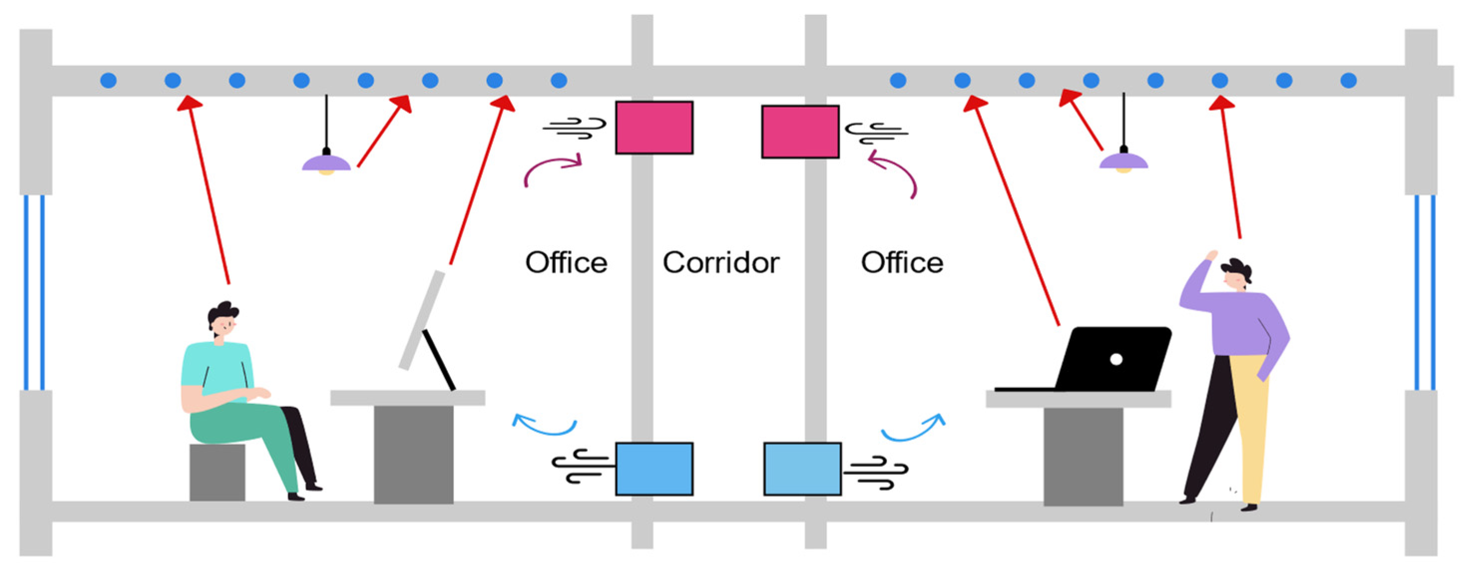
The research method was divided into two parts, one was the physical simulation model establishment of radiant ceiling cooling room (as shown in Figure 1), and the other was the modeling of control methods. The traditional on–off and PID control methods could be implemented through the components in TRNSYS simulation software.
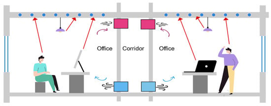
Figure 1.
Schematic diagram of radiant ceiling cooling room model.
3.1.1. Simulation Environment
Compared to more developed HVAC systems, environmental control simulations for radiant ceiling cooling systems were relatively rare. Currently, more and more high-end office buildings were beginning to use radiant panels for cooling. Based on standard office buildings in reality and combined with local actual weather data, a room model was established. The room structure, cooling load, and radiant panel selection were considered in the establishment of the physical model to ensure that the design met the specifications, as seen in Section 3.2.
3.1.2. Control Methods
The traditional on–off control and PID control method could be achieved using the environment simulation software TRNSYS, as demonstrated in Section 3.3. The learning-based control method, which took the combination of deep learning (DL) and reinforcement learning (RL), could be achieved with programming software Python 3.8, as demonstrated in Section 4.
3.2. Physical Model of Room
3.2.1. Meteorological Data
The simulation software used in this study was TRNSYS, which has a variety of integrated meteorological data reading modules. We used meteorological modules in IWEC format, and the meteorological data source was the national meteorological data collection official website energyplus.net (accessed on 20 April 2021). The time of cooling load calculation was from 06-01 00:00:00 to 10-01 00:00:00 in data, and the corresponding annual simulation period was 3624 h to 6552 h.
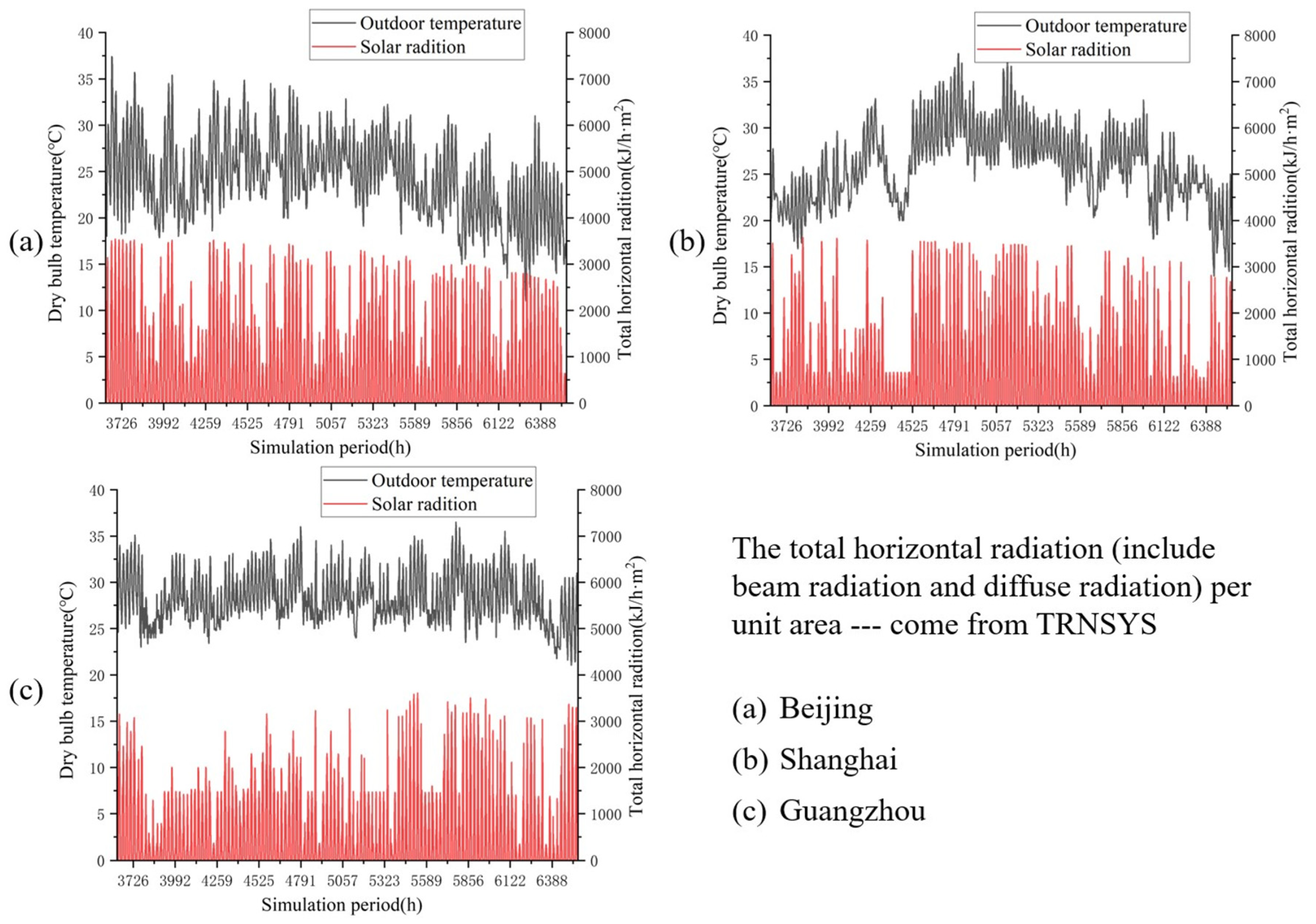
In this simulation, three different building regions in China were selected: Beijing, Shanghai and Guangzhou, which, respectively, corresponded to the cold region, hot summer and cold winter region, and hot summer and warm winter region. Outdoor temperature and solar radiation varied curves in different regions are shown in Figure 2.
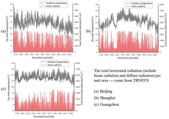
Figure 2.
Outdoor climatic parameters in different cities.
3.2.2. Room Structure
Two standard office rooms facing south and north in a typical office building were selected as the research object. The room had only one exterior wall with one window and the room specification structure is shown in Figure 3. The room’s length, width and height were 5.5 m, 3.4 m and 2.8 m, and the window’s length and high was 3.0 m and 1.65 m (window frame occupying 15% of the total area).

Figure 3.
Office room specifications.
The thermal performance parameters of enclosure structure were determined according to the relational national standard in China [24,25], as shown in Table 1. The thickness of the thermal insulation layer for the external walls in Shanghai was 25 mm and there was no thermal insulation layer for the external walls in Guangzhou.

Table 1.
Relevant enclosure structure parameters.
3.2.3. Room Cooling Load
The room cooling load calculation part mainly included four parts: (1) the heat transferred through the enclosure, (2) the solar radiation heat entered through the window, (3) the human body heat dissipation, and (4) the indoor equipment heat dissipation. With a cycle of one week, the time of workers’ occupancy in the room and the running time of indoor equipment are shown in Figure 4.

Figure 4.
Time of occupant and equipment operation.
Based on the cooling load calculations using TRNSYS18, the maximum sensible heat load for both rooms in each region were obtained (see Table 2). It should be noted that solar radiation had clear effect on room cooling loads due to different windows’ orientation.

Table 2.
Statistics of sensible heat load calculation.
3.2.4. Radiant Panel Selection
In order to ensure indoor healthy, the radiant ceiling cooling system was usually used together with a dedicated outdoor air system. The supply air temperature and air volume rate were set as 20 °C and 30 m3/h per person, and the indoor relative humidity was kept at 50%. Since the supply air temperature was lower than the indoor temperature, the supply air would take part of the room cooling load, so this part needed to be removed for the selection of radiant panel. The specific selection of radiant panels and some related data are shown in Table 3.

Table 3.
Design and selection of radiant panel.
In the TRNSYS model, the construction of radiant panels was completed through the construction of the ‘Chilled ceiling’ layer in the ‘Layers’ of the ‘Construction Types’ in the multi-zone building model. In addition, two contact modes of ceiling radiant panel and ceiling were given: (1) the structure with air interlayer and (2) the structure with direct attachment and tight connection. The first type was adopted in the study, which could effectively prevent the upward cooling loss through the air interlayer.
3.3. Simulation Modeling of Traditional Control Models
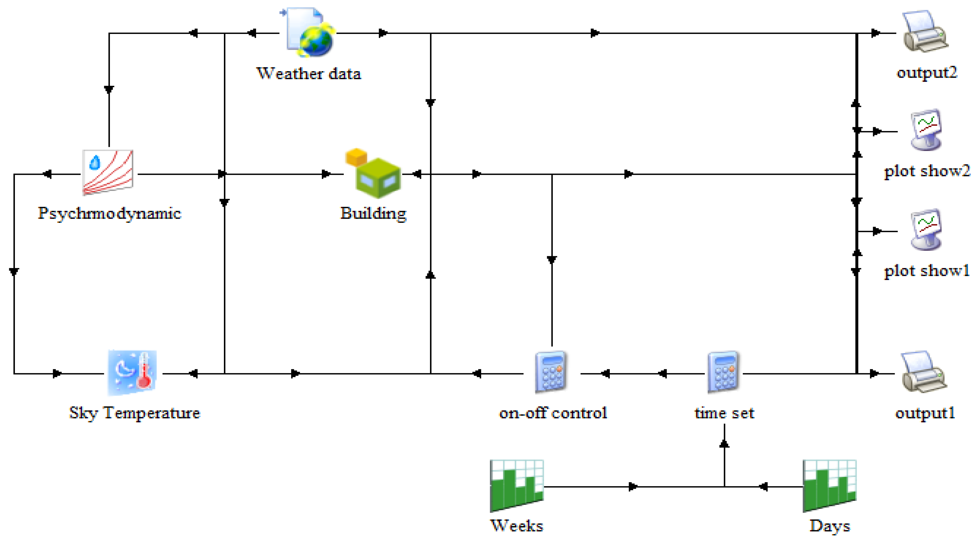
We used TRNSYS to establish the control simulation models, as shown in Figure 5 and Figure 6. The establishment of different traditional control method models is shown in the following parts. The simulation module of the model mainly included: the weather data module, the wet air calculation module, the sky temperature calculation module, the building heat balance calculation module, the simulation time operation function setting module (weeks, days), the visual output module (output, plot show), and the control module. The building heat balance calculation module was the core of this simulation, which mainly included the energy balance calculation of the building room and various designed heating, ventilation, and air conditioning systems. Other modules provided boundary conditions and control conditions for building heat balance calculation. Among them, the meteorological parameter module provided various relevant weather parameters of the region, and the wet air calculation module provided the relative humidity and dry bulb temperature and the sky temperature calculation module provided the equivalent sky temperature. The calculation control module played different roles in different models according to the edited algorithm. The controls for the simulation were only active during the working hours. They were turned on one hour in advance to ensure that the room temperature met the requirements when the workers entered.

Figure 5.
TRNSYS simulation model for traditional on–off control.
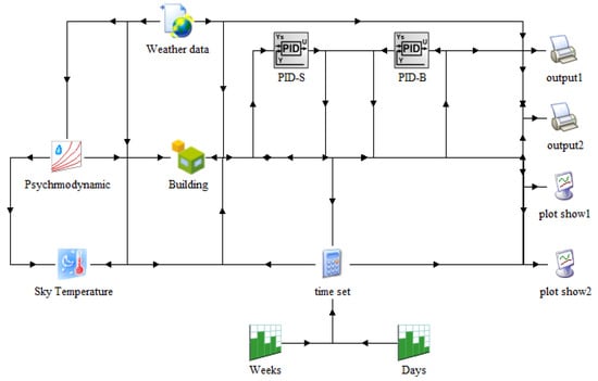
Figure 6.
TRNSYS simulation model for PID variable water temperature control.
3.3.1. Traditional on–off Control Model of Radiant Ceiling Cooling System
The traditional on–off control was realized through the on–off control module, and the digital signals of 0 and 1 were output to the ‘Building’ module to control the opening and closing of the supply water valves in the two rooms. Among them, the valve control during the working period was realized through the simulation time operation function setting module (weeks, days). When setting the target indoor temperature control, the lower limit of the target indoor temperature for on–off control was 26 °C. Once the indoor temperature dropped below 26 °C during the working time, the valve was forced to close. The supply water temperature and supply water flow of the on–off control model were kept at constant, and only the opening and closing of the supply water valve were controlled.
3.3.2. PID Variable Water Temperature Control Model of Radiant Ceiling Cooling System
The PID variable water temperature control module was implemented through type 23 in TRNSYS, with a control target of the indoor temperature of 26 °C only during working hours. The supply water temperature of radiant ceiling cooling system was adjusted through the opening of the mixing valve to get the required water temperature. The supply water flow of the PID control model was a fixed value, and the parameter output of the PID control was the supply water temperature. The variable range of the supply water temperature was 17.0–26.0 °C (the lower limit was the design supply water temperature, and the upper limit was the indoor target temperature).
The proportional coefficient determined the speed of the system’s response. Adjusting the proportional term could quickly improve the accuracy of the system, but it could not eliminate steady-state errors. Therefore, an integral term was needed, but its size needed to match the inertia of the designed radiant ceiling cooling system and consider the system’s response time. If the inertia was large, the effect of the integral term should be weaker and the integral time should be increased. The differential term could determine the trend of error changes and make adjustments in advance, thereby speeding up the system’s response and reducing adjustment time. Therefore, the improvement of PID control performance was closely related to the parameter tuning of the three terms. The final results of PID parameter tuning for two rooms in each region are shown in Table 4.

Table 4.
PID setting parameters.
4. Simulation Modeling of DRL Control Model
This study intended to employ the DRL method to control the radiant ceiling cooling room, which required a combination of reinforcement learning (RL) and deep learning (DL). RL emphasized the interaction between the control model and the surroundings, while DL focused on data analysis and processing. This control method was developed through external programming software Python and communicated with TRNSYS’s room physical model through the bridging, as shown in Figure 7. The following described the specific logical process and the corresponding modeling process of DRL.
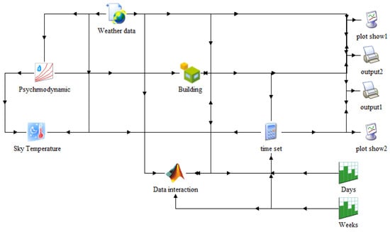
Figure 7.
TRNSYS simulation model for DRL interaction.
4.1. DRL Control Model of Radiant Ceiling Cooling System
In order to achieve data exchange with the DRL model established in the Python programming software, the Data Interaction module (type155) was added to the TRNSYS model. The ‘Data interaction’ module obtained the environmental state parameters during the operation process of the physical model in the ‘Building’ module and transferred them to the DRL model as input parameters. Then through the ‘Data interaction’ module, the DRL model exported the feedback action instructions into the room model. Two different DRL control simulations were conducted: (1) DRL controlled the opening and closing of the supply water valve and (2) DRL controlled the changes in supply water temperature, and compared them separately with two traditional control methods (Section 3.3).
In this study, we used MATLAB as a connecting bridge by communicating through m-files written in MATLAB to interact the information between simulated environments. The action instructions and environmental parameters considered in each simulation were different. By modifying the MATLAB m-file called by the type155 module, different simulation requirements could be met. The DRL model established different control logic for different simulations and discreteness the action instructions into different dimensional vectors. For on–off control simulation, only two action instructions (open and close) were available. For water temperature control simulation, the range of supply water temperature was discredited into 19 variable actions at intervals of 0.5 °C between 17 °C and 26 °C.
4.2. Reinforcement Learning (RL) Process
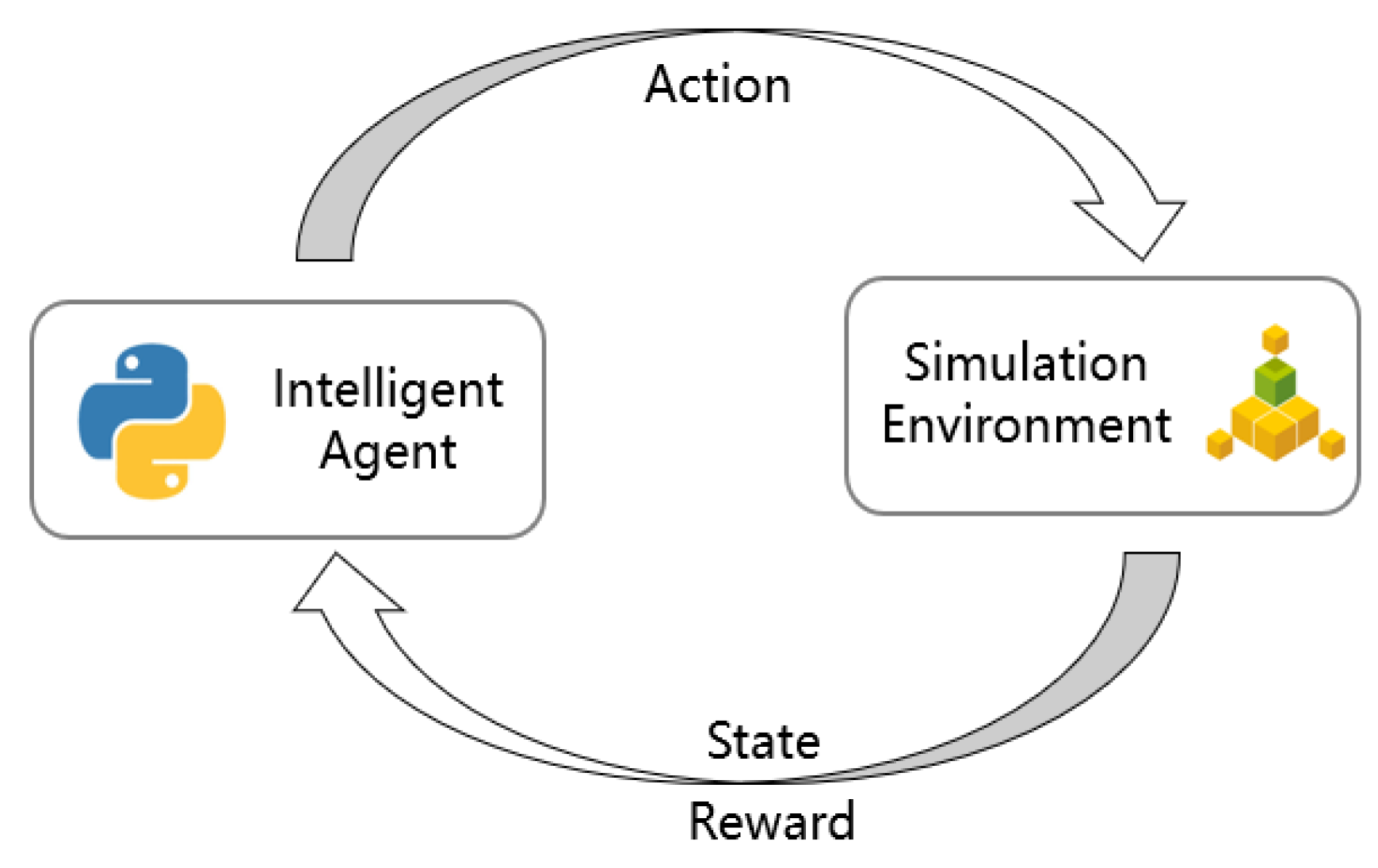
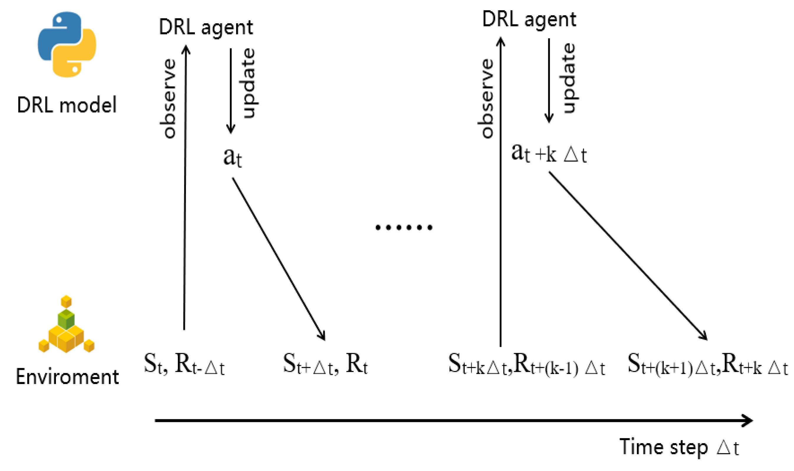
The radiant ceiling cooling system needed to maintain the indoor temperature as the target set temperature with the varied external environmental parameters, such as the current indoor temperature and external environmental solar radiation, supply water temperature, radiation panel temperature, and other disturbances. The indoor temperature for the next step could be determined by the current system state and environmental disturbances as well as the input supply water temperature and flow rate. It could be independent of the previous state of the building. Therefore, the control of a radiant ceiling cooling system could be seen as a Markov reinforcement learning process [26], as shown in Figure 8.

Figure 8.
Diagram of reinforcement learning process.
(1) Environment state: Determining the next optimal action based on the observation of the current state of the simulation environment. This step considered the interference of selected parameters such as indoor temperature and external environmental factors that were input into the DRL model. In order to be closer to the actual situation and reflect the impact of real weather on regulation, authoritative data published by the National Meteorological Administration were selected and gradually reflected in the simulation environment according to the time series.
(2) Control method: The supply water temperature and supply water valve of the radiant panel were adjustable, and the state of the supply water valve had two options: S = {open, close}. The supply water temperature could be selected from multiple discrete levels, represented by T = {t1, t2,…, tm}. If control was performed using two action variables, then the entire output space would be n = 2 × m. If there were too many rooms and the supply water temperature was discredited more finely, the dimension of the action space would rapidly increase, which would increase the training time and make convergence difficult, ultimately reducing control performance. Therefore, the simulation compared the control of the supply water valve and supply water temperature separately, rather than controlling them together.
(3) Reward: The goal was to control the indoor temperature within a specified target range. Based on our action state space A = {a1, a2,…}, after performing an action in the previous state St−1, the environment changed to a new state St, ready for the next action. At this point, a mechanism was needed to evaluate the performance of this action and provide rewards or punishments.
The design of the reward and punishment strategy had an important impact on the speed and control results of the reinforcement learning algorithm. The calculation not only included the reward® of the current action but also the cumulative rewards of all previous actions to achieve the best training effect. We could use a rewarded discount factor γ [0, 1] to represent how much the current action affected future rewards. When γ = 1, future rewards were considered equally important as immediate rewards. The above Equation (1) was a state value function, representing the sum value (Vπ) of all discounted rewards from a certain state St until the end of the sampling period. However, the expected target output influenced by the action value was considered, as shown in Equation (2).
The state transition of buildings was random and could not be accurately measured due to the influence of environmental interference. Therefore, the best Q value estimation would be updated according to the Q learning method, as shown in Equation (3).
where indicated the learning rate. Larger could speed up the convergence, but the effect was not necessarily good. Smaller could make the algorithm stable, but would prolong the training time [8]. Specific control is shown in Figure 9 [21].
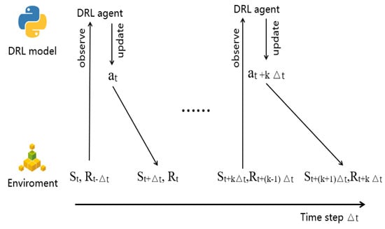
Figure 9.
DRL algorithm control building flow chart.
4.3. Deep Learning (DL) Process
In this paper, we used not the general DQN but the improved Double DQN in our simulation. Compared to policy-based methods (DDPG, AC, PPO), value-based methods (Double DQN) can only handle discrete actions but have a relatively lower computational cost for training. This is because policy-based methods require maintaining separate networks for action and critic, while value-based methods solely rely on the Bellman equation and only need to calculate the Q network during iteration. Value-based methods are effective in smaller action spaces [27] and Q-learning has been shown to be effective in slow thermodynamic systems such as radiation [22].
The Q-learning algorithm stored the “action-value” pairs in a table and was a Markov decision process about discrete state and action spaces. However, in practical problems, various possible combinations of actions and states formed a large-scale state and action space, which could cause the disaster of dimensionality in general reinforcement learning and make computation difficult. Generalization methods that used random trees and neural networks to approximate Q-values were usually effective. In the simulation, a weighted ω neural network was used to approximate the value function Q(s,a,ω). However, function approximations had the risk of instability and divergence, especially for nonlinear approximations such as neural networks. However, by using experience replay and learning methods that determined target Q-values, neural networks were proven to be effective and stable. The purpose of deep neural networks was to solve how to obtain Q-values faster and more efficiently in a large state space.
The simulation considered input state parameters such as solar radiation, supply and return water temperature, indoor dry bulb temperature, outdoor temperature, supply air temperature, wind speed, and other observable parameters. Some non-dimensional parameters would be obtained through standardization and vector distance algorithms with the target state. The more observed state parameters that were considered and the closer they were to reality, the greater the challenge to DRL and the more practical significance it had.
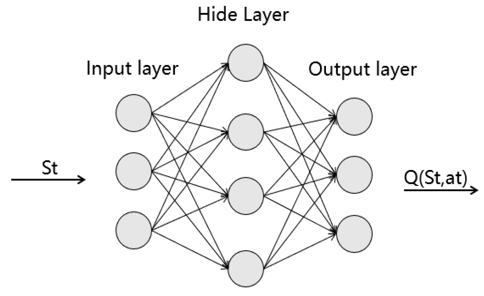
According to the neural network structure (as shown in Figure 10), the Q-value of all control actions could be directly obtained through the hierarchical transmission of the neural network after the state St input, which could greatly improve the efficiency of the greedy algorithm or ‘softmax’ selection. ‘ReLU’, as the activation function of the hidden layer, was output at the last fully connected linear layer. The deep neural network needed a lot of data for training, and it required independent distribution between samples. However, the sample size obtained by the reinforcement learning agent was sparse and had a certain delay, and the sample obtained was also continuous. Therefore, it was necessary to establish a data storage unit for the DL part of the DRL model to store historical environmental interaction and action data.
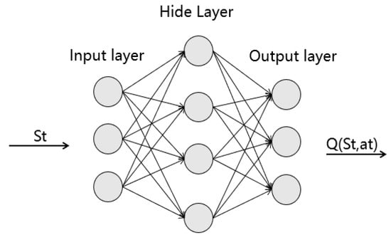
Figure 10.
Neural network structure.
To solve the problems caused by the combination of deep neural networks and reinforcement learning, two key points were summarized:
(1) Sample pool (experience replay): The state samples collected by the agent were put into a sample pool, and then random samples were taken from the sample pool for training. This approach broke the correlation between samples, making them independent and solving the problem of non-stationary distribution. Through the sample pool, the neural network could learn from current and previous experiences, which improved learning efficiency.
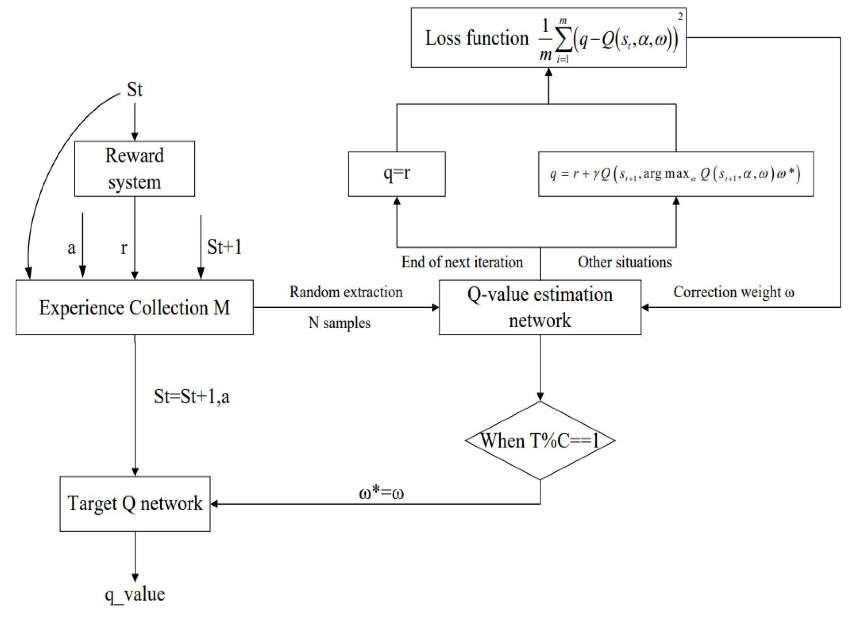
(2) Fixed Q-target network: Perturbation mechanism for Q-value correlations. To compute the target value of the network, existing Q-values were used. Using a slower-updating network to provide this Q-value could improve algorithm stability and convergence. The Q-target introduced two Q-value outputs in the algorithm, both using the same neural network but with different input parameters. The predicted Q-value input the current state, while the target Q-value input the old state. The mean square error Formula (4) was used to obtain the error loss between the current Q-value and the target Q-value, which was then used to update the weight parameters ω.
The target Q-value of the update process Q* could be obtained by Equation (5) when the gradient decreased, and the predicted Q value could be approximated by neural network.
4.4. DRL Control Model Algorithm Design
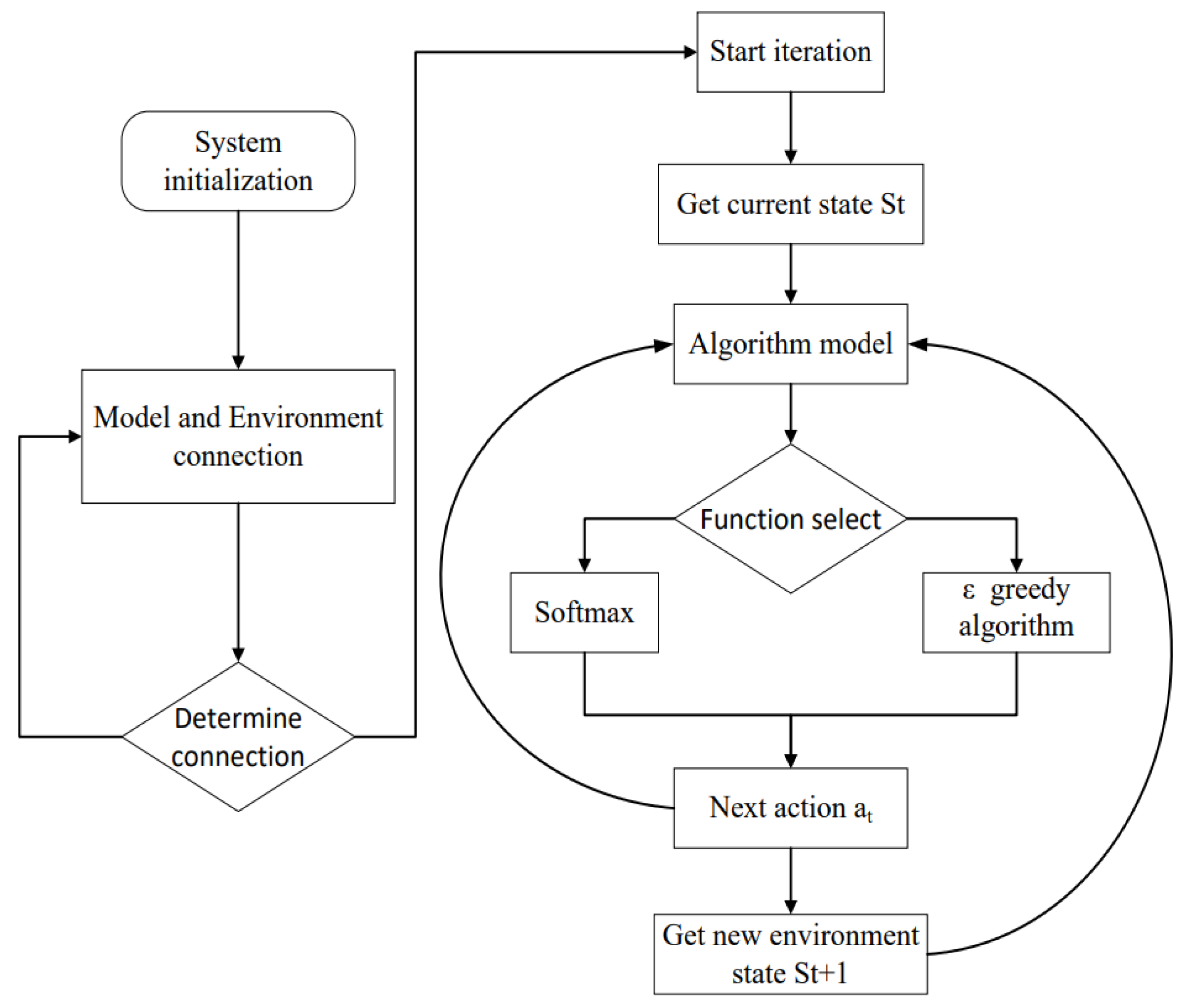
The runtime simulation environment continuously carried out state feedback according to the action instructions to improve the control strategy. The control time length of the environment determined the training times of an iteration. The algorithm updated the batch and time step according to the environment settings. The DRL model consisted of a cyclic process of interaction with the environment and an internal self-learning optimization process, as shown in Figure 11 and Figure 12.
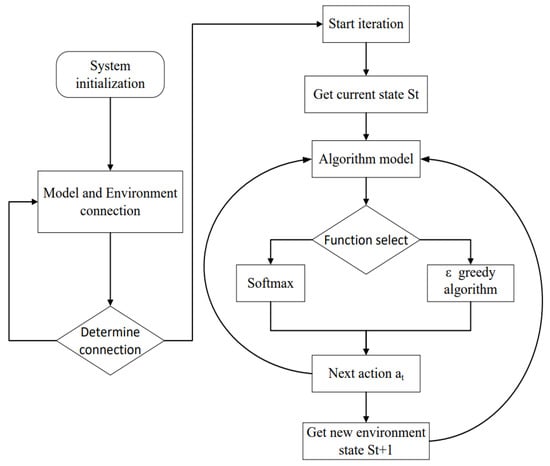
Figure 11.
Algorithm flow diagram of DRL and environment interaction.
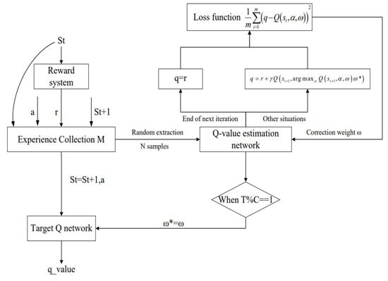
Figure 12.
Internal circulation flow diagram of DRL.
Initialization setting: Firstly, the number of iteration rounds T, the characteristic dimension n of characteristic states St, and the algorithm of reward R and rewarded discount factor γ were determined. If you use ε, the greedy algorithm was also needed to determine the exploration rate ε, Q network structure, update network frequency C and randomly initialize Q network weight parameters ω. Also noted was that for the experience replay storage set M, each recent transition tuple (St, At, Rt, St−1) would be pushed into M and continuously extracted, initialized as an empty set, and set its size reasonably. The total number of layers of the neural network was 3. Of course, compared to some large network models, it was relatively shallow. The specific process was as follows.
- Initialize all parameters of Q network ω, Target Q* network ω* = ω, and Random-based ω. Initialize states and actions and corresponding q-value. Clear the experience playback collection M.
- Ensure the normal connection between the algorithm model and the environment, and reset the environment to the initial state.
- When the communication connection was smooth and the environment was running normally, carry out the iteration.
- (1)
- Obtain the current state quantity of environment initialization, and conduct preliminary processing to obtain the characteristic state parameter S.
- (2)
- In the Q network, take S as the input to obtain the action output of all corresponding q-values of the Q network, and the ε Greedy algorithm or ‘softmax’ selected the corresponding action ‘a’ from the current q-value (the ‘softmax’ function performed well in the simulation).
- (3)
- Execute the action ‘a’ in the current state St, and obtain the processed characteristic state vector St+1 of the new environment state and the reward r of this action.
- (4)
- Put tuples (St, a, St+1, r) into experience replay storage set M.
- (5)
- Assignment: St = St+1.
- (6)
- Randomly select n samples from the experience replay set M, and calculate the target q-value of these samples to update the Q-value estimation network.
- (7)
- (8)
- The weight value ω was modified by the loss function
As a fast response system, the radiant ceiling cooling system would consider the impact of recent actions on future response during control, so the rewarded discount factor γ would be set at a higher value, and the internal parameters are shown in Table 5. The reward and punishment strategy of DRL considered the indoor temperature of the controlled room.

Table 5.
Internal parameters of DRL algorithm.
In order to maximize the control effect of the DRL model in the radiant ceiling cooling system, the DRL reward and punishment strategy were set and optimized before comparison and verification. During the simulation of strategy optimization, many detailed mathematical algorithms and the evaluation design of the temperature control range was carried out, and the simulation data after several different strategy modifications were processed. The final selection is shown in Table 6, where Δt in the following table represented the temperature difference with the set control target set T (26 °C). The specific evaluation mathematical language and rewards and punishment values were not given in the Table 6.

Table 6.
DRL reward and punishment strategy.
5. Results
The comparison simulation was divided into two parts: (1) comparison of DRL on–off with traditional on–off control method and (2) comparison of DRL variable water temperature with PID variable water temperature control method.
5.1. Comparison of DRL on–off with Traditional on–off Control Method
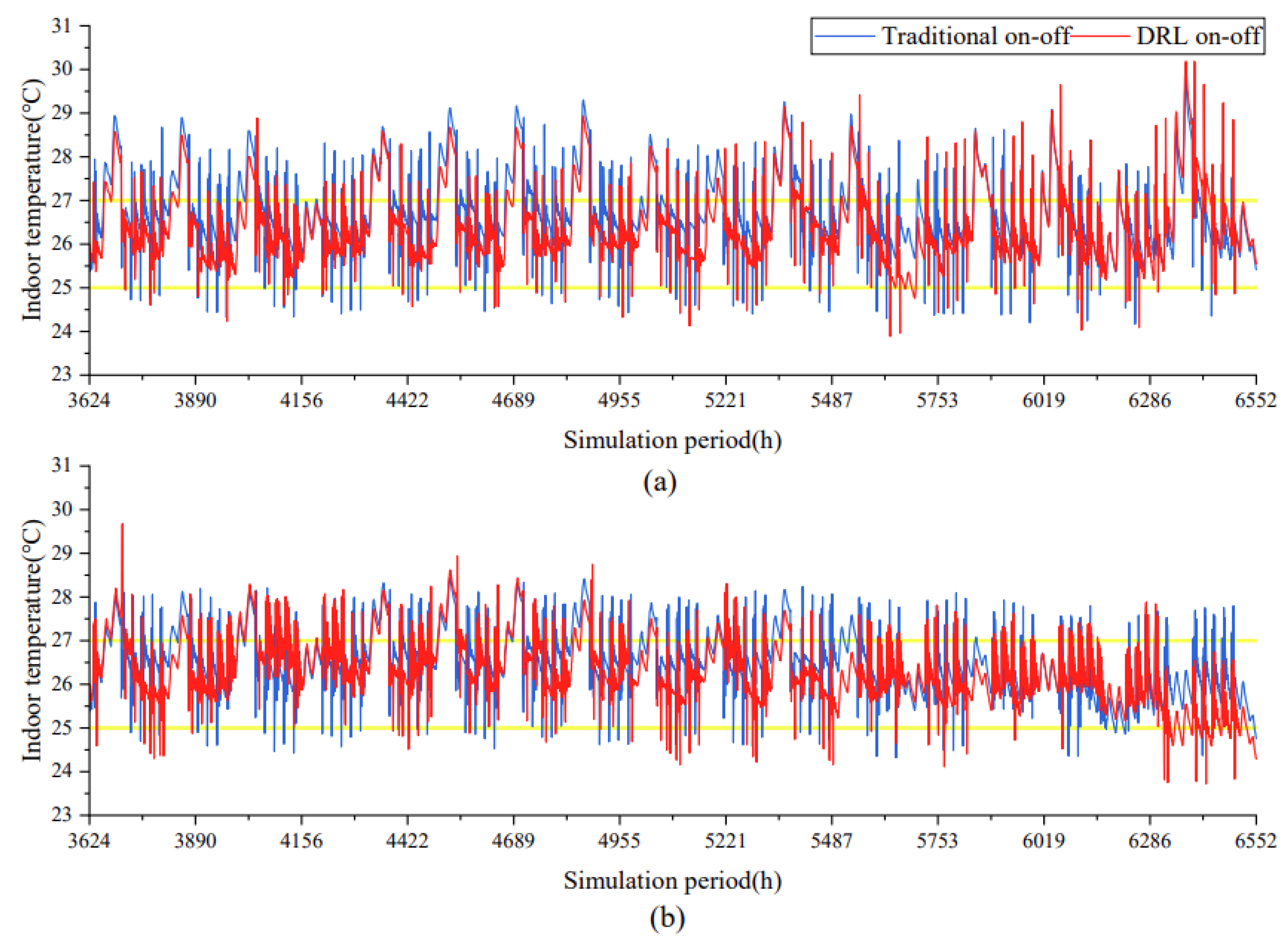
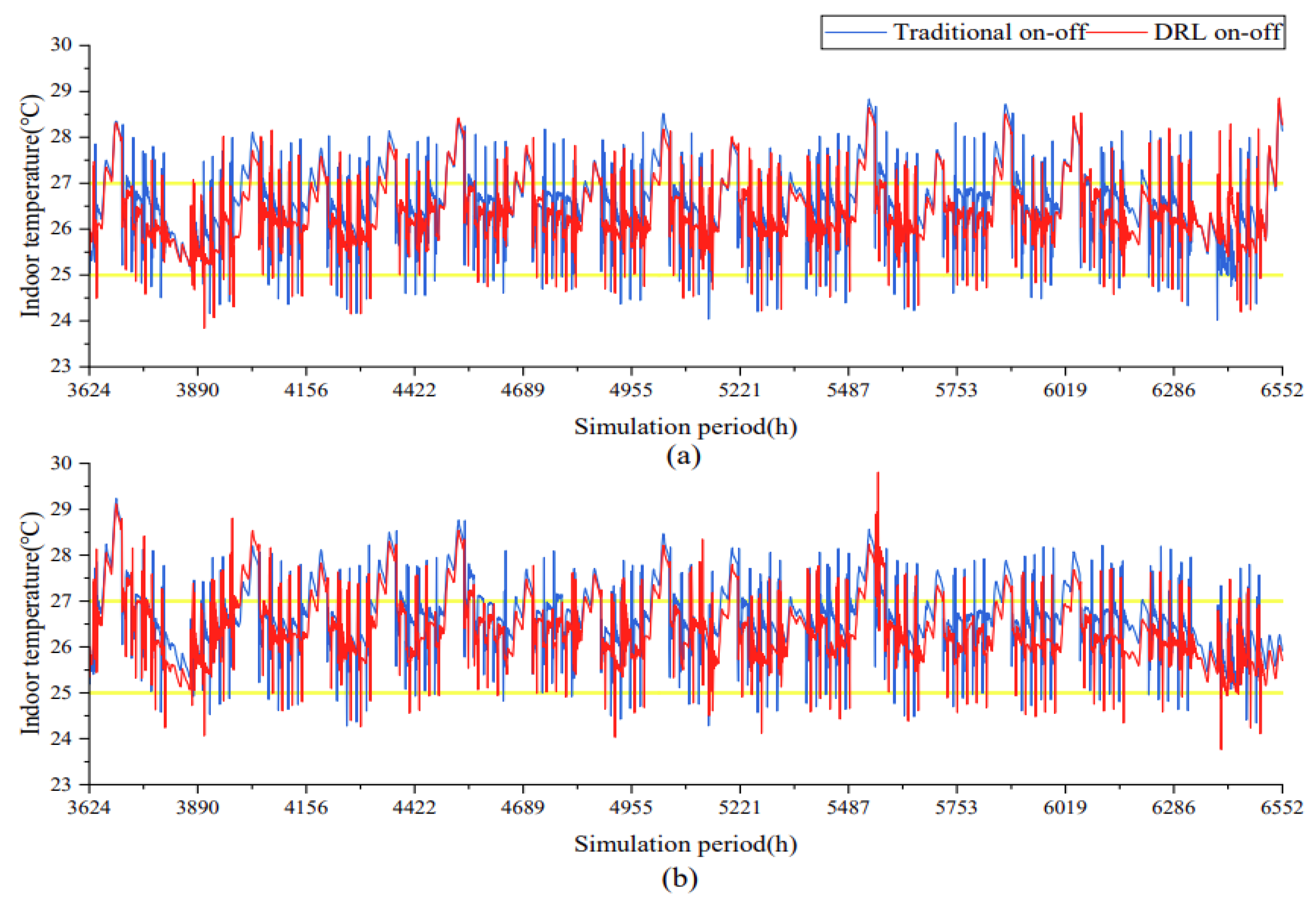
DRL on–off and traditional on–off control method were used to control the opening and closing of the supply water valve, and the indoor temperature varied curves in two rooms in each city are shown in Figure 13, Figure 14 and Figure 15.
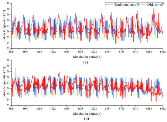
Figure 13.
Indoor temperature varied curve of on-off control in Beijing ((a) south-facing room, (b) north-facing room).
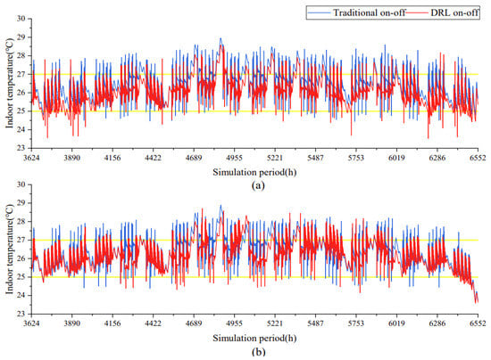
Figure 14.
Indoor temperature varied curve of on-off control in Shanghai ((a) south-facing room, (b) north-facing room).
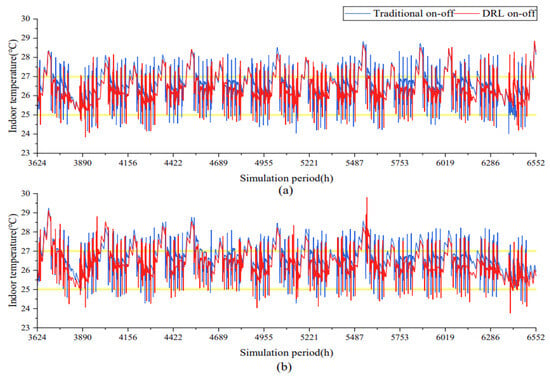
Figure 15.
Indoor temperature varied curve of on-off control in Guangzhou ((a) south-facing room, (b) north-facing room).
Figure 13, Figure 14 and Figure 15 indicated the observed indoor temperature fluctuation patterns. The DRL on–off control method trained with a target temperature of 26 °C nearly had the same control effect as the traditional on–off control, but the controlled indoor temperature with DRL on–off method was generally lower compared to the traditional on–off method. Moreover, both control methods could ensure that the indoor temperature fluctuated within the allowable range of 25–27 °C during the work time (between the two yellow lines), but each operation would cause a one-time up-and-down oscillation of the indoor temperature due to the on–off control of the supply water valve, unless we found a suitable valve on-time ratio based on the thermal inertia of the room [28].
Although on–off control could cause indoor temperature oscillations, the temperature oscillation with DRL on–off control was clearly better than that with traditional on–off control, as shown in Figure 13, Figure 14 and Figure 15. The further comparisons of temperature control effects and energy consumption could be seen in Figure 16 and Figure 17.
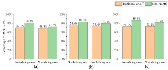
Figure 16.
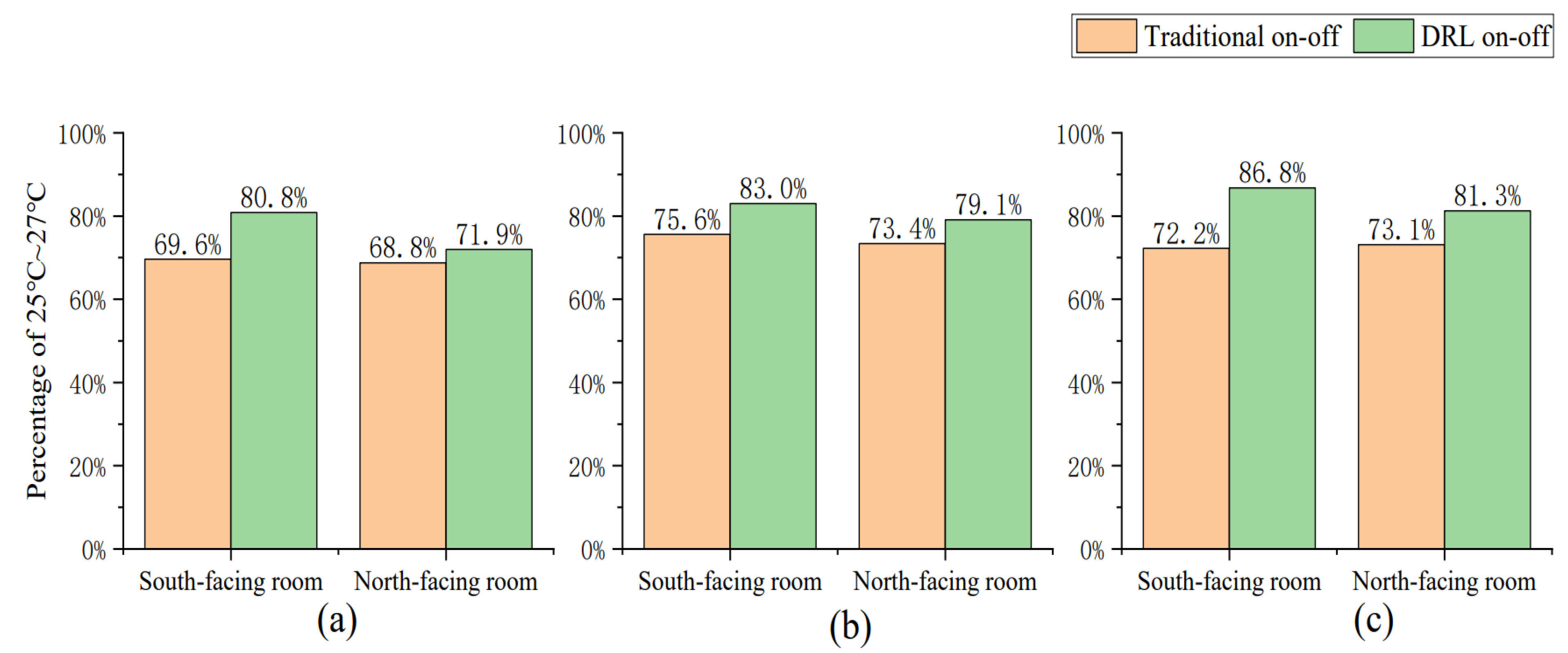
Statistical chart of indoor temperature of on-off control ((a) Beijing, (b) Shanghai, (c) Guangzhou).
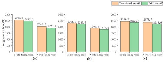
Figure 17.
Statistical chart of energy consumption of on-off control ((a) Beijing, (b) Shanghai, (c) Guangzhou).
As shown in Figure 16, considering the cumulative work time of 688 h, the indoor temperature percentage of 25–27 °C with the DRL on–off control was significantly higher than the traditional on–off control in two rooms in three cities. Moreover, the DRL on–off control ensured that the requirements for indoor temperature fluctuations were met almost 80% of the work time, while the traditional on–off control only satisfied this requirement about 70% of the work time. Due to a wide range of permissible temperature, the enhanced comfort effect of indoor temperature was not significant among different cities and orientations. However, north-facing rooms generally had a less improvement in indoor temperature control compared to south-facing rooms. This might probably because that south-facing room experienced intense solar radiation, which limited the effectiveness of traditional or DRL on–off control. Climate change was a difficult problem for the traditional on–off control, but DRL model could be trained to adapt to the climate change.
Figure 17 indicated that the DRL on–off control had lower energy consumption compared to the traditional on–off control in both south-facing and north-facing rooms in three cities. In addition, compared with the traditional on–off control, the energy consumption with DRL on–off control can be saved from 3.19% to 6.30%. According to the actual energy-saving values of different rooms, the maximum saved energy consumption appeared in the north-facing rooms, and the minimum always appeared in the south-facing rooms. The different orientations of rooms would absorb solar radiation with different magnitude and frequency, and the south-facing rooms significantly absorbed more solar radiation than the north-facing rooms. Solar radiation was uncontrollable disturbance to the DRL model training, and the stronger the external disturbance, the more challenging the training becomes.
5.2. Comparison of DRL Variable Water Temperature with PID Variable Water Temperature Control Method
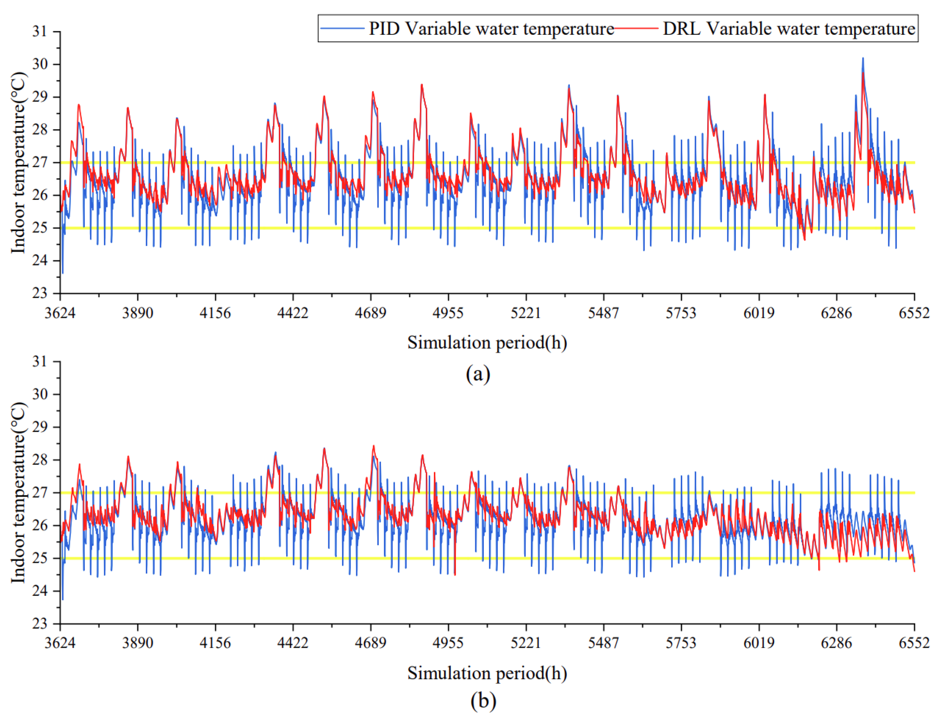
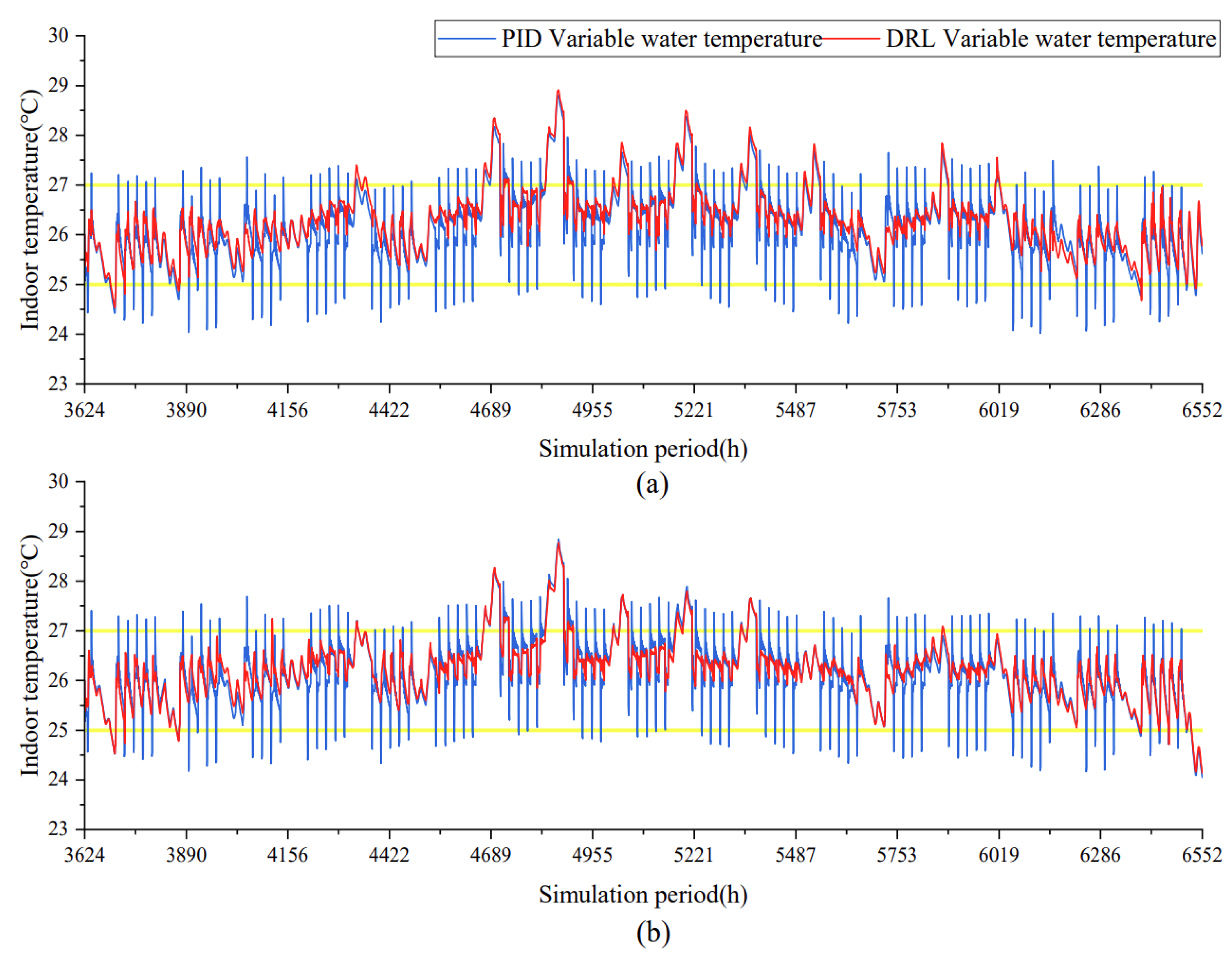
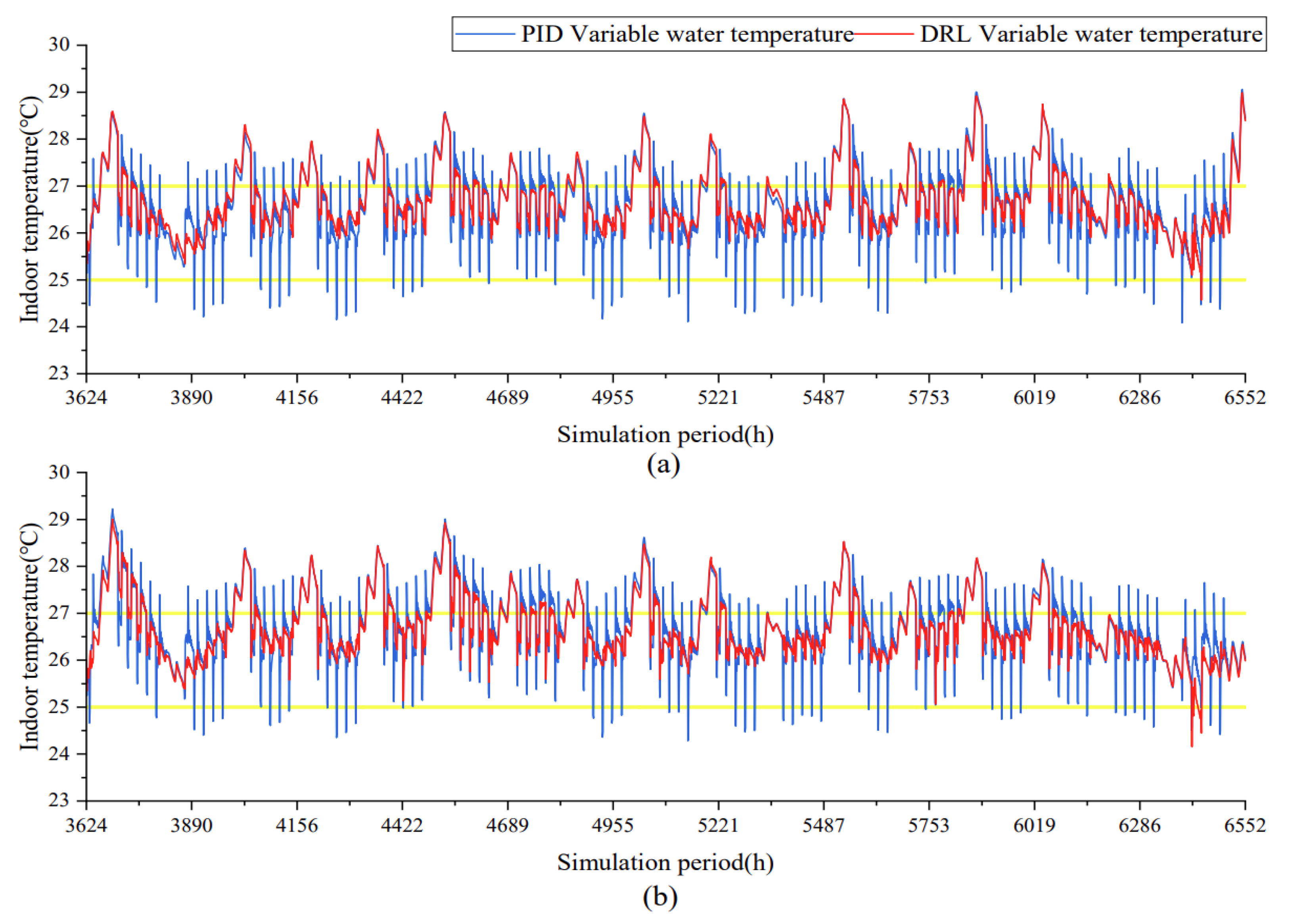
The indoor temperature varied curves in two rooms in each city with DRL and PID variable water temperature control method are shown in Figure 18, Figure 19 and Figure 20.
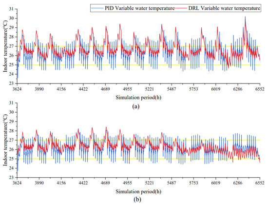
Figure 18.
Indoor temperature varied curve of variable water temperature control in Beijing ((a) south-facing room, (b) north-facing room).
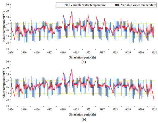
Figure 19.
Indoor temperature varied curve of variable water temperature control in Shanghai ((a) south-facing room, (b) north-facing room).
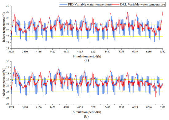
Figure 20.
Indoor temperature varied curve of variable water temperature control in Guangzhou ((a) south-facing room, (b) north-facing room).
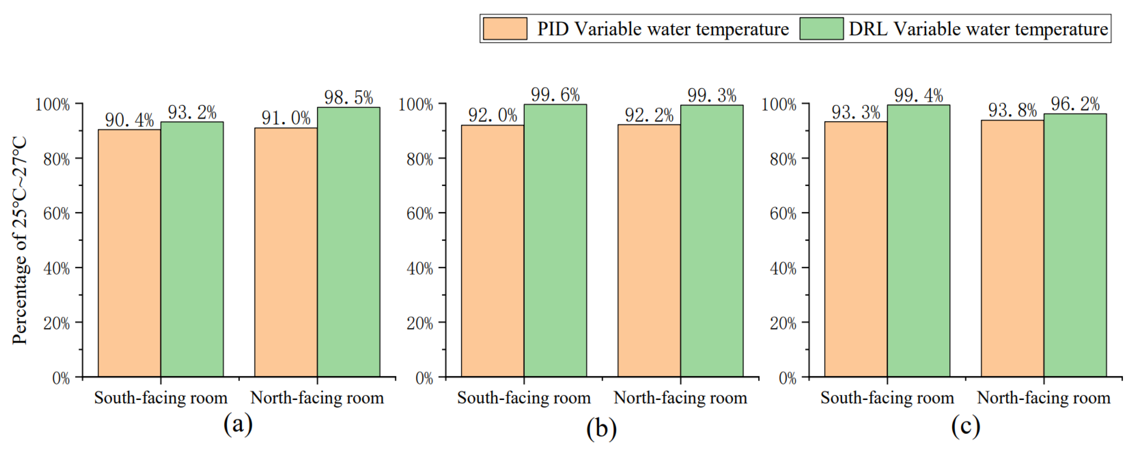
As shown in Figure 18, Figure 19 and Figure 20, DRL control caused fluctuations with relatively small amplitude and low frequency in indoor temperature, while PID control resulted in large amplitude and high frequency oscillations. Moreover, both control methods almost ensured the indoor temperature within the allowable temperature range of 25–27 °C during the work time. However, the PID control would experience a period of temperature oscillation after opening the supply water valve at the initial few hours during each working period, which was the overshoot adaptation process of the PID control before stabilizing [29]. The temperature oscillation would have an impact on indoor thermal comfort in practical applications, so in addition to achieving its objectives, stability was also crucial for a control method. The further statistical results of indoor temperature control and energy consumption with DRL and PID variable water temperature control methods are shown in Figure 21 and Figure 22.
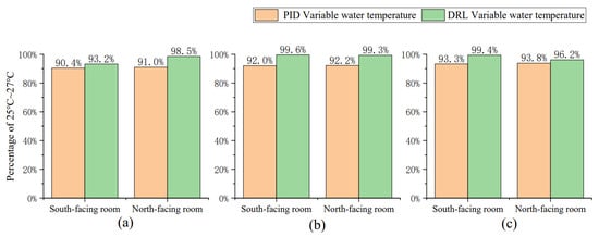
Figure 21.
Statistical chart of indoor temperature of variable water temperature control ((a) Beijing, (b) Shanghai, (c) Guangzhou).
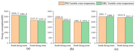
Figure 22.
Statistical chart of energy consumption of variable water temperature control ((a) Beijing, (b) Shanghai, (c) Guangzhou).
Figure 21 indicated that the indoor temperature control effect with DRL variable water temperature control in two rooms in three cities was slightly better than that with PID control. Moreover, the DRL control could ensure 93% to 99% of the work time within the allowable temperature fluctuation range, while the PID control only ensure 90% to 93% of the work time is comfortable. Although PID control caused temperature oscillations, its oscillation time was not long, and the overall thermal comfort level was close to the DRL control. Figure 21 also shows that the control effects in Shanghai with DRL control were better than in Beijing and Guangzhou. This might be due to the different solar radiation and thermal performance parameters of building envelopes in three cities. From the perspective of outdoor parameter changes, Beijing had the large fluctuation and Guangzhou had the small. The overall performance of DRL and PID control in Beijing was indeed poor compared to the other two cities (see Figure 16 and Figure 21). Nevertheless, DRL still successfully achieved its control objectives and indicated good robustness.
As shown in Figure 22, energy consumption of radiant ceiling cooling system with DRL method was slightly smaller than that with PID method. The energy-saving effect of DRL compared with PID was not very obvious, except in the simulation in the south-facing room in Shanghai (see Figure 22b), where the energy-saving benefit increased by 10.48%. To avoid accidental results, the study was conducted through multiple simulations, and each simulation result for the north-facing room in Shanghai was very similar. Moreover, DRL showed different energy saving effects in simulations of different rooms in different regions, which was worth considering and leading to not effective results by analyzing the weather factors in different regions or the differences in the physical models of the rooms. However, by comparing the results of multiple DRL controls, DRL was relatively more energy efficient than PID for each simulation.
6. Discussion
6.1. Performance of the DRL Method
In this study, two control methods were evaluated for the radiant ceiling cooling system: a simple on–off control approach and a more complex variable water temperature control method. Both traditional control and the DRL method were implemented for these control methods. The two control methods had distinct action state spaces, resulting in varying environmental states following different actions. However, the DRL method demonstrated positive outcomes in both control scenarios, as shown in Table 7.

Table 7.
Comparative effectiveness of DRL methods.
The DRL on–off control method demonstrated superior thermal comfort levels and lower energy consumption when compared to the traditional on–off control approach. The indoor temperature curve with DRL on–off control exhibited a smoother fluctuation pattern, with smaller amplitude and duration, in contrast to the traditional on–off control. However, the DRL on–off control method required slightly more frequent opening and closing of the supply water valve compared to the traditional method. Under identical conditions, the opening and closing frequency of the supply water valve with the traditional on–off control varied from 500–580 times, depending on the city and orientation. In comparison, the DRL on–off control method showed an increase in the opening and closing frequency ranging from 20–60 times higher than the traditional method. Although this increased frequency is a trade-off associated with the DRL on–off control, the impact on the entire cooling season is relatively small.
Based on the analysis of the indoor temperature variation, temperature control effectiveness, and energy consumption results, it was found that the DRL variable water temperature control method outperformed the PID variable water temperature control method for the radiant ceiling cooling system. Although the energy savings achieved by the DRL method compared to the PID method were not substantial, the impact on reducing indoor temperature fluctuations was significant.
6.2. Analysis of the DRL Method
The simulation results indicated variations in the effectiveness of optimization control in radiant ceiling cooling rooms with different orientations in various regions. It can be inferred that the disparities in temperature control and energy-saving outcomes may be significantly influenced by the specific model employed, and in certain regions, the optimization may not have been fully achieved. Additionally, the parameters of distinct physical models and control output parameters can also contribute to these discrepancies. Furthermore, when the same DRL model was implemented in rooms facing different directions, divergences in simulation results may arise due to differing external disturbances in different regions.
Based on the simulation results using on–off control, the DRL method demonstrated better improvement in indoor temperature control for the south-facing room compared to the north-facing room. However, the actual energy savings achieved were somewhat lower. When variable water temperature control was employed, the DRL method did not exhibit the same pattern, and its overall optimization performance was inferior to on–off control. These findings suggest that there may be limitations to the optimization capabilities of the DRL method when applied to different control output parameters.
Differences in simulation results can also arise from variations in the configuration of reward and punishment strategies. This study made multiple adjustments to the reward and punishment strategy. However, during the process of optimizing the strategy, certain strategies that were logically superior performed worse in practical application. This discrepancy can be attributed to two factors: (1) inadequate research on reward and punishment strategies, and (2) limitations in maximizing the control of supply water in the radiant ceiling cooling system. Due to space constraints and the depth of the research, the comparative outcomes of different reward and punishment strategies were not presented in this paper. Nonetheless, the experimentation resulted in the selection of one of the most effective reward and punishment strategies.
7. Summary and Future Work
7.1. Summary
This study compared the performance of DRL control method with that of the traditional on–off control method and PID variable water temperature control method for radiant ceiling cooling systems. The system simulation results were analyzed to determine the optimal control approach for such systems. The findings indicate that the DRL on–off control method outperformed the traditional on–off control method in terms of reduced indoor temperature fluctuations and energy consumption. Moreover, the DRL variable water temperature control method demonstrated superior performance compared to the PID variable water temperature control method for radiant ceiling cooling systems. These results suggest that the DRL control method has significant potential for energy savings and operational efficiency in radiant ceiling systems. As computer technology and artificial intelligence continue to advance, the DRL control method may replace traditional control methods in the future.
7.2. Future Work
The design of reward and punishment strategies in the field of HVAC is a crucial issue, particularly for achieving automated improvements through the DRL model. While researchers have made attempts to apply various algorithms to HVAC systems, the role of HVAC expertise in this context should be emphasized. In this study, preliminary tests were conducted on several strategies, which yielded relatively good results. However, there is still ample room for improvement in terms of control effectiveness, as well as potential for exploring new research directions. Future work will focus on enhancing the optimization and selection process of the DRL model, as well as refining the reward and punishment strategies. Additionally, further research is warranted to consider the thermal inertness of the radiant ceiling cooling system, as well as its integration with a mechanical ventilation system. To facilitate these investigations, an experimental bench has been established, and it is anticipated that the simulation will be implemented in practical applications in the future.
Author Contributions
Methodology, Z.L.; Software, J.L.; Validation, Z.T.; Data curation, J.X.; Writing–original draft, M.T.; Writing–review & editing, J.G.; Project administration, X.W. All authors have read and agreed to the published version of the manuscript.
Funding
This study was funded by National Natural Science Foundation of China (Grant No. 52278091 & 51978429).
Conflicts of Interest
The authors declare no conflict of interest.
References
- China Association of Building Energy Efficiency. China Building Energy Consumption Research Report 2020. J. Build. Energy Effic. 2021, 49, 30–39. (In Chinese) [Google Scholar]
- Department of Energy. Buildings Energy Data Book. 2011. Available online: https://ieer.org/wp/wp-content/uploads/2012/03/DOE-2011-Buildings-Energy-DataBook-BEDB.pdf (accessed on 20 April 2021).
- EIA. Energy Consumption Survey (CBECS). 2012. Available online: http://www.eia.gov/tools/faqs/faq.cfm?id=86&t=1 (accessed on 10 April 2021).
- Oyedepo, S.O.; Fakeye, B.A. Waste heat recovery technologies: Pathway to sustainable energy development. J. Therm. Eng. 2021, 7, 324–348. [Google Scholar] [CrossRef]
- Afram, A.; Janabi-Sharifi, F. Theory and Applications of HVAC Control Systems–A Review of Model Predictive Control (MPC). Build. Environ. 2014, 72, 343–355. [Google Scholar] [CrossRef]
- Cho, S.-H.; Zaheer-Uddin, M. An Experimental Study of Multiple Parameter Switching Control for Radiant Floor Heating Systems. Energy 1999, 24, 433–444. [Google Scholar] [CrossRef]
- Song, D.; Kim, T.; Song, S.; Hwang, S.; Leigh, S.B. Performance Evaluation of a Radiant Floor Cooling System Integrated with Dehumidified Ventilation. Appl. Therm. Eng. 2008, 28, 1299–1311. [Google Scholar] [CrossRef]
- Meng, Z.Y.; Yu, G.Q.; Jin, R. Design of PID Temperature Control System Based on BP Neural Network. Appl. Mech. Mater. 2014, 602–605, 1244–1247. [Google Scholar] [CrossRef]
- Jin, A.; Wu, H.; Zhu, H.; Hua, H.; Hu, Y. Design of Temperature Control System for Infant Radiant Warmer Based on Kalman Filter-fuzzy PID. J. Phys. Conf. Ser. 2020, 1684, 12140. [Google Scholar] [CrossRef]
- Zhao, J.; Shi, L.; Li, J.; Li, H.; Han, Q. A Model Predictive Control Regulation Model for Radiant Air Conditioning System Based on Delay Time. J. Build. Eng. 2022, 62, 105343. [Google Scholar] [CrossRef]
- Zhang, D.; Huang, X.; Gao, D.; Cui, X.; Cai, N. Experimental Study on Control Performance Comparison between Model Predictive Control and Proportion-integral-derivative Control for Radiant Ceiling Cooling Integrated with Underfloor Ventilation System. Appl. Therm. Eng. 2018, 143, 130–136. [Google Scholar] [CrossRef]
- Dong, B.; Lam, K.P. A real-time model predictive control for building heating and cooling systems based on the occupancy behavior pattern detection and local weather forecasting. Build. Simul. 2014, 7, 89–106. [Google Scholar] [CrossRef]
- Pang, X.; Duarte, C.; Haves, P.; Chuang, F. Testing and Demonstration of Model Predictive Control Applied to a Radiant Slab Cooling System in a Building Test Facility. Energy Build. 2018, 172, 432–441. [Google Scholar] [CrossRef]
- Joe, J.; Karava, P. A Model Predictive Control Strategy to Optimize the Performance of Radiant Floor Heating and Cooling Systems in Office Buildings. Appl. Energy 2019, 245, 65–77. [Google Scholar] [CrossRef]
- Chen, Q.; Li, N. Model Predictive Control for Energy-efficient Optimization of Radiant Ceiling Cooling Systems. Build. Environ. 2021, 205, 108272. [Google Scholar] [CrossRef]
- Liu, Q.; Zhai, J.; Zhang, Z.; Zhong, S.; Zhou, Q.; Zhang, P.; Xu, J. A summary of deep reinforcement learning. J. Comput. Sci. 2018, 41, 1–27. (In Chinese) [Google Scholar]
- Albert, B.; May, M.; Zadrozny, B.; Gavalda, R.; Pedreschi, D.; Bonchi, F.; Cardoso, J.; Spiliopoulou, M. Autonomous HVAC Control, A Reinforcement Learning Approach. In Machine Learning and Knowledge Discovery in Databases; Lecture Notes in Computer Science; Springer International AG: Cham, Switzerland, 2015; Volume 9286, pp. 3–19. [Google Scholar]
- Li, B.; Xia, L. A Multi-grid Reinforcement Learning Method for Energy Conservation and Comfort of HVAC in Buildings. In Proceedings of the 2015 IEEE International Conference on Automation Science and Engineering (CASE), Gothenburg, Sweden, 24–28 August 2015; pp. 444–449. [Google Scholar]
- Zenger, A.; Schmidt, J.; Krödel, M. Towards the Intelligent Home: Using Reinforcement-Learning for Optimal Heating Control. In KI 2013: Advances in Artificial Intelligence; Springer: Berlin/Heidelberg, Germany, 2013; pp. 304–307. [Google Scholar]
- Zhang, Z.; Chong, A.; Pan, Y. A Deep Reinforcement Learning Approach to Using Whole Building Energy Model for HVAC Optimal Control. In Proceedings of the 2018 Building Performance Modeling Conference, Chicago, IL, USA, 26–28 September 2018. [Google Scholar]
- Wei, T.; Wang, Y.; Zhu, Q. Deep Reinforcement Learning for Building HVAC Control. In Proceedings of the 54th ACM/EDAC/IEEE Design Automation Conference (DAC), Austin, TX, USA, 18–22 June 2017. [Google Scholar]
- Blad, C.; Koch, S.; Ganeswarathas, S.; Kallesøe, C.S.; Bøgh, S. Control of HVAC-systems with Slow Thermodynamic Using Reinforcement Learning–ScienceDirect. In Proceedings of the 29th International Conference on Flexible Automation and Intelligent Manufacturing (FAIM2019), Limerick, Ireland, 24–28 June 2019. [Google Scholar]
- Ding, Z.; Pan, Y.; Xie, J.; Wang, W.; Huang, Z. Application of reinforcement learning algorithm in air-conditioning system operation optimization. J. Build. Energy Effic. 2020, 48, 14–20. (In Chinese) [Google Scholar]
- GB 55015-2021; General Code for Energy Efficiency and Renewable Energy Application in Buildings. National Standard of China; China Architecture & Building Press: Beijing, China, 2021.
- GB 50189-2015; Design Standard for Energy Efficiency of Public Buildings. National Standard of China; China Architecture & Building Press: Beijing, China, 2015.
- Gao, G.; Li, J.; Wen, Y. DeepComfort: Energy-Efficient Thermal Comfort Control in Buildings Via Reinforcement Learning. IEEE Internet Things J. 2020, 7, 8472–8484. [Google Scholar] [CrossRef]
- Jiang, Z.; Risbeck, M.J.; Ramamurti, V.; Murugesan, S.; Amores, J.; Zhang, C.; Lee, Y.M.; Drees, K.H. Building HVAC control with reinforcement learning for reduction of energy cost and demand charge. Energy Build. 2021, 239, 110833. [Google Scholar] [CrossRef]
- Liu, L.; Fu, L.; Jiang, Y. An On-off Regulation Method by Predicting the Valve On-time Ratio in District Heating System. Build. Simul. 2015, 8, 665–672. [Google Scholar] [CrossRef]
- Janprom, K.; Permpoonsinsup, W.; Wangnipparnto, S. Intelligent Tuning of PID Using Metaheuristic Optimization for Temperature and Relative Humidity Control of Comfortable Rooms. J. Control Sci. Eng. 2020, 2020, 2596549. [Google Scholar] [CrossRef]
Disclaimer/Publisher’s Note: The statements, opinions and data contained in all publications are solely those of the individual author(s) and contributor(s) and not of MDPI and/or the editor(s). MDPI and/or the editor(s) disclaim responsibility for any injury to people or property resulting from any ideas, methods, instructions or products referred to in the content. |
© 2023 by the authors. Licensee MDPI, Basel, Switzerland. This article is an open access article distributed under the terms and conditions of the Creative Commons Attribution (CC BY) license (https://creativecommons.org/licenses/by/4.0/).

