Abstract
This article presents a study on the mechanical properties and constitutive model of Dahurian larch wood under parallel-to-grain (ParG) and perpendicular-to-grain (PerG) cyclic loading. A total of twenty-four dog-bone specimens were designed and prepared. Failure modes, stress–strain curves, elastic moduli under monotonic loading, and unloading/reloading moduli under cyclic loading were analyzed. Results indicated that the tensile and compressive envelope curves of wood under cyclic loading are similar to the monotonic stress–strain curves. The unloading and reverse reloading stiffness of wood are significantly degraded in both material directions. Furthermore, a constitutive model that is capable of considering the degradation of cyclic compression unloading stiffness and the change in reverse compression (tension) stiffness after tension (compression) unloading was proposed. A comprehensive comparison with test results was conducted, and they are in good agreement. Thus, the correctness of the proposed constitutive model is verified.
1. Introduction
Wood has been applied to the construction industry for thousands of years due to its easy processing features [1,2,3]. In recent years, it has again been gaining increasingly widespread applications in modern timber structures for many advantageous reasons, such as environmental friendliness, a high strength–weight ratio, architectural aesthetics, etc. Wood is a heterogeneous material, causing highly anisotropic mechanical properties [4,5]. Thus, improving fundamental understanding of the mechanical properties of wood is a mandatory task and could foster the structural application of wood.
Wood has three principal material axes, namely the longitudinal (L), radial (R), and tangential (T) directions. The mechanical properties and stress–strain curves of wood highly depend on the loading directions. The modulus of elasticity, shear modulus, and Poisson’s ratio are the commonly used elastic constants of wood. Comprehensive studies have also investigated the influence of structural characteristics and physical properties on the elastic constants of wood [6,7,8].
A reliable constitutive model of wood is necessary for the effective mechanical analysis of timber structures. In recent years, many data-dependent and theoretical constitutive models have been proposed, such as the empirical model, the elastic–plastic model, and the damage model. The empirical constitutive model of wood has been commonly used in theoretical and numerical analyses of timber elements. However, it cannot fully describe the nonlinear full-process mechanical behavior of wood, so the nonlinear characteristics of the timber elements cannot be well described. In recent years, researchers have successively developed an elastic–plastic constitutive model and an elastic–plastic damage constitutive model based on continuum mechanics. The problem caused by the empirical constitutive model was preliminarily solved. Oudjene [9] and Guan [10] proposed an elastic–plastic constitutive model to reflect the plastic densification effect of wood under transverse compression based on Hill and Tsai-Wu strength criteria, respectively. Chen et al. [11] and Yang et al. [12] established an elastic–plastic constitutive model. Based on continuum damage mechanics, three-dimensional elastic damage constitutive models of wood were proposed by Sandhaas et al. [13], Gharib et al. [14], Eslami et al. [15], and Arruda et al. [16], and elastic–plastic damage constitutive models by Sirumbalzapata et al. [17], Wang et al. [18], Benvenuti et al. [19], and Zhang et al. [20].
The above constitutive models are proposed for the normal service environment and quasi-static stress conditions of wood. In order to further expand the application of wood constitutive models, Chen et al. [21] introduced a multi-linear reduction model to include the influence of temperature on the mechanical properties of wood. Jiang et al. [22] proposed a constitutive model to describe the long-term interaction of wood under different temperature, humidity, and load conditions. Zhang et al. [23] established a three-dimensional dynamic elastic–plastic damage constitutive model of wood considering the effect of high strain rates under dynamic loading. Yu et al. [24] proposed a comprehensive 3D constitutive rheological model to consider orthotropic, elastic–plastic, viscoelastic, and mechano-sorptive aspects, including the complex mechano-sorptive recovery phases that may occur over the lifetime.
The above research results provide basic data for the numerical analysis of timber structures and greatly improve the capability and reliability of the results. However, there are still many problems that need in-depth investigation, especially for timber structures that may be subjected to cyclic actions such as seismic and fatigue loadings [20]. Therefore, it is urgent to investigate the cyclic mechanical behavior and constitutive model of wood. It should be noted that in recent years, some scholars have preliminarily developed the cyclic compression properties of wood along and across grain and established corresponding constitutive models. For instance, Xie et al. [25] and Edzang et al. [26] carried out cyclic compression research on Dahurian larch and tropical wood, respectively. However, the cyclic loading was limited to the compression side without considering the tensile side. Zhang et al. [27] reported the fatigue failure and deformation characteristics of aging timber specimens under constant-amplitude alternating cyclic loading. Although the loading involved both tension and compression sides, the purpose was to explore the relationship between the upper limit stress ratio and the number of cycles within the elastic range, not the cyclic mechanical behavior of wood after the elastic range. It can be seen that previous studies have not investigated the loading and unloading stiffness degradation behavior of wood under a full loading process when the load changes from tension to compression and from compression to tension. There is also a lack of a hysteretic constitutive model considering the cyclic characteristics of wood.
In this paper, the mechanical properties and constitutive model of wood under cyclic loading are presented. The deformation mode, damage characteristics, and change law of important mechanical indexes of wood were analyzed, and a constitutive model capable of describing the behavior of wood under cyclic loading was established. The research results provide a good reference for the numerical analysis and mechanical evaluation of timber structures.
2. Materials and Methods
2.1. Material and Specimens
The commonly used wood species in Chinese traditional timber structures, Dahurian larch (Larix gmelinii Rupr.), was adopted. Its density, moisture content, and average annual ring width were determined as 413 kg/m3, 13.2%, and 0.82 mm according to GB/T 1927.3 [28], GB/T 1927.4 [29], and GB/T 1927.5 [30], respectively.
The shapes and sizes of the ParG and PerG compressive specimens specified in the existing mechanical testing standards for wood [31,32,33] cannot be directly used, and special designing is required. The dog-bone specimen used by Zhang et al. [27] when testing the cyclic tension and compression fatigue properties of wood has been referenced and modified to avoid premature instability through multiple experimental and numerical tests, as shown in Figure 1. The effective length of the specimen is 20 mm, and its cross-section size is 10 mm × 10 mm. All the specimens were fabricated by an experienced carpenter according to GB/T-1927.2 [34]. A serious vision inspection was conducted before preparation to avoid macroscopic defects such as decay, knots, wormholes, etc., according to GB-50005 [35].
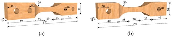
Figure 1.
Specimen configuration (unit: mm). (a) ParG specimen. (b) PerG specimen.
A total of twenty-four specimens were prepared and classified into six groups, as shown in Table 1. Before testing, all the samples were adjusted in standard room conditions with temperatures of 20 ± 2 °C and relative humidity of 65% ± 5% according to GB/T-1927.5 [28] to reach approximately 12% moisture content.

Table 1.
Grouping of the wood specimens.
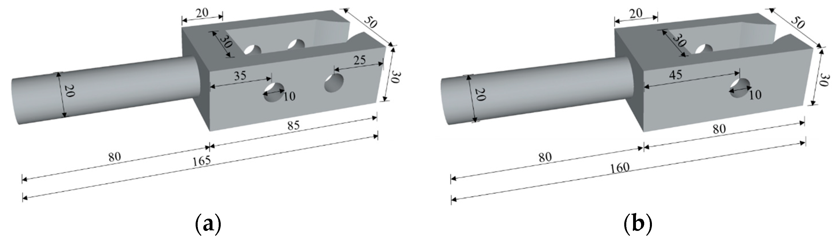
When the loading head of the testing machine is clamping the wood specimen, there will be a relatively large lateral pressure imposed on the specimen to avoid its slip. The lateral pressure may exceed the transverse compressive strength of the wood, so it is not possible to directly clamp the specimen using the self-contained clamp. In order to avoid the failure of the clamping section of the specimen before the end of the cycle loading, a transition connection device between the specimen and the clamp is specially designed. The shapes and sizes of the transition connection devices designed for ParG and PerG specimens are shown in Figure 2.
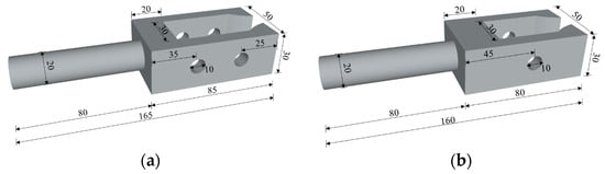
Figure 2.
Specimen fixtures (unit: mm). (a) ParG specimen fixture. (b) PerG specimen fixture.
2.2. Loading Scheme
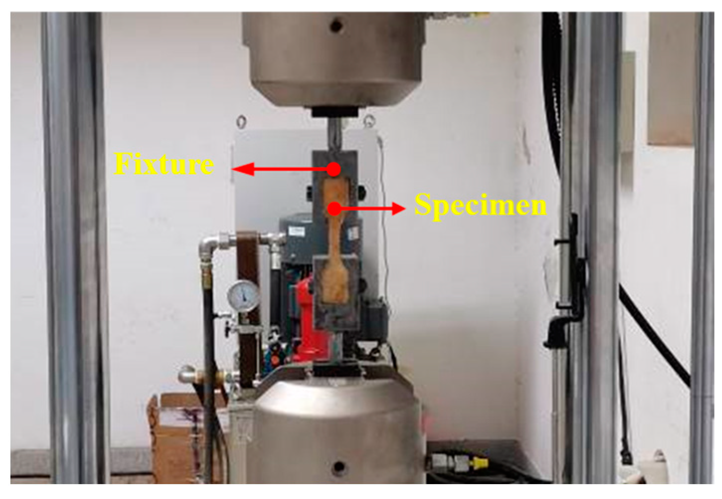
The test was carried out on an SDS100 electro-hydraulic servo fatigue testing machine, and the loading device is shown in Figure 3.

Figure 3.
Test setup.
The specimens and the fixtures were fabricated with high accuracy and can be closely assembled. The displacement control loading scheme is adopted, and the loading rate is 1.0 mm/min and 0.8 mm/min for ParG and PerG specimens, respectively. The cyclic loading schemes for the ParG and PerG specimens are shown in Figure 4. There are 5 cyclic cycles and 4 cyclic cycles for ParG and PerG loading cases, respectively. To avoid tensile failure of PerG wood specimens, a maximum tensile stress of 3 MPa is controlled. The displacement and load are automatically recorded by the test machine.
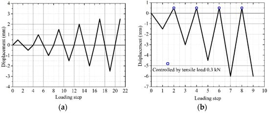
Figure 4.
Cyclic loading schemes. (a) ParG specimens. (b) PerG specimens.
3. Test Results and Analysis
3.1. Failure Mode
3.1.1. Parallel-to-Grain Tension
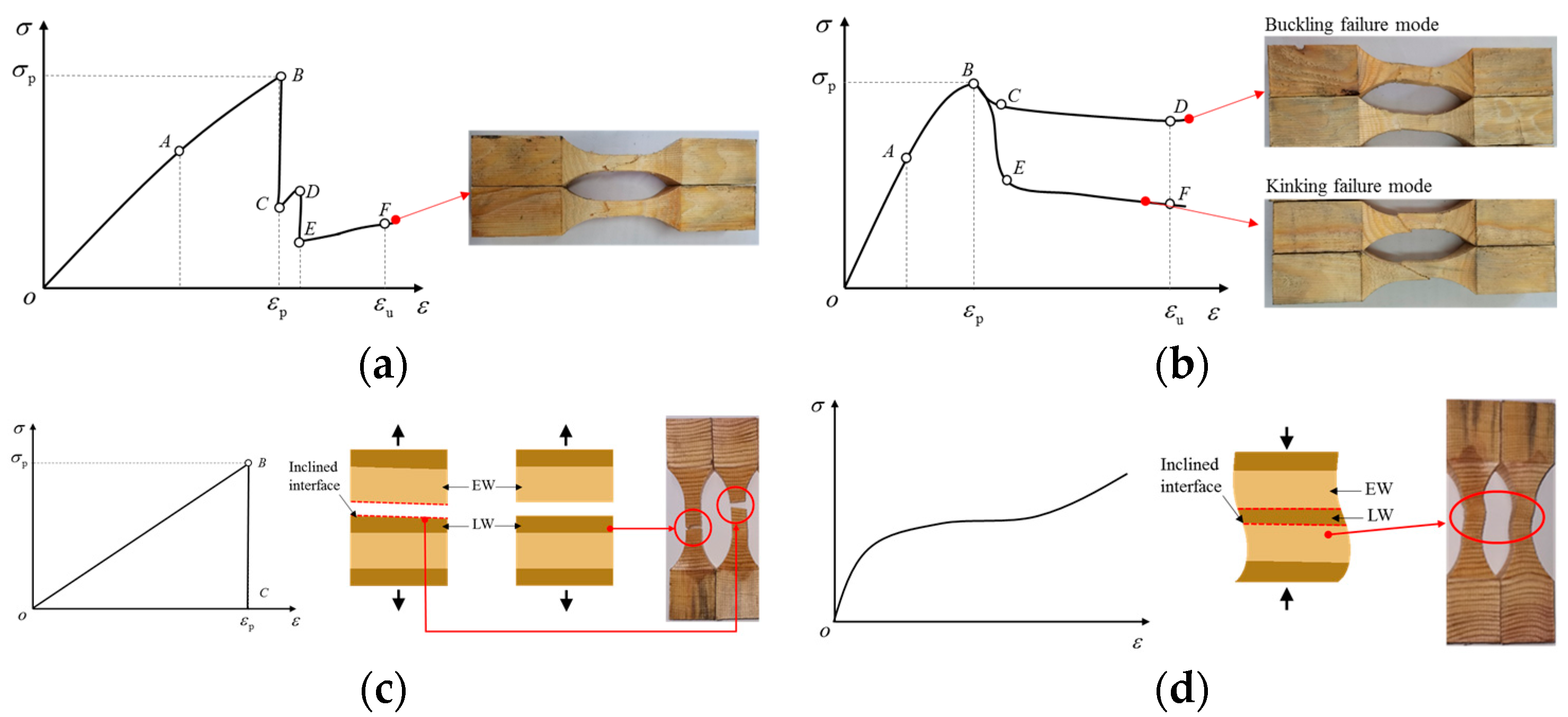
The ParG tensile and compressive failure mechanisms and failure modes of wood under both monotonic and cyclic loading are shown in Figure 5. It can be seen that the tensile process includes two stages divided by the peak point B, namely the stable tensile stage (OB) and the random progressive tensile fracture stage (BF).

Figure 5.
Failure modes of wood. (a) ParG tension. (b) ParG compression. (c) PerG tension. (d) PerG compression.
As the load linearly increases to peak point B, the initial defects within the wood begin to expand, and local wood fibers begin to fracture and sometimes emit a fiber fracturing sound. At this time, only a portion of the microfibers break, and there are no visible cracks on the specimen surfaces. Once reaching peak point B, the number of local fractures in wood fibers increases, gradually connects to form broken fiber bundles, and produces obvious local fracture areas on specimen surfaces. Stress drops occur (see branch BC in Figure 5a). It is worth noting that the fracture position and stress drop amplitude of the fiber bundle at the effective stress branch are usually random variables, depending on the internal wood microstructure and the distribution of growth defects.
The local fiber bundle fracture of the wood does not mean the failure of the whole specimen because it can continue to bear the load. The subsequent mechanical behavior is related to the performance of the remaining effective fiber bundles; thus, the stress slowly increases with the increase in strain (see Figure 5a). At point D, the strain of the remaining effective section gradually increases, and the next random fracture of the fiber bundle continues to occur. The stress once again drops in branch DE and continues to be felt in branch EF. The specific drop value is also a random variable.
3.1.2. Parallel-to-Grain Compression
The failure modes of wood under monotonic and cyclic compression are shown in Figure 5b. It can be seen that the compression process of wood parallel to the grain is more complex than that under tension. The ParG compression stress–strain curve can be divided into the linear segment (OA) and nonlinear segment (AB) before the peak point. After peak point B, two typical deformation modes can be observed according to the shape of the stress–strain curves and the failure process of the specimens. The first deformation mode is the compression buckling failure mode, with the stress after the peak point decreasing smoothly and slowly with the increase in load (B-C-D segment). The second deformation mode is characterized by the shear failure mode, in which the stress drops suddenly and then slowly decreases with the increase in load (B-E-F segment).
3.1.3. Perpendicular-to-Grain Tension and Compression
The parallel-to-grain tensile and compressive failure mechanisms and failure modes of wood under both monotonic and cyclic loading are shown in Figure 5. It shows the PerG tensile and compressive failure modes of wood. Brittle failure was evidently observed in the tensile tests. Two types of morphology of the exposed fracture surfaces can be noted depending on whether the interface of the early wood (EW) and late wood (LW) was inclined (see Figure 5c). The PerG compression deformation modes of wood present buckling characteristics due to the unevenness of the EW and LW (see Figure 5d). During the PerG compression process, the softer parts in the same wood area are damaged first, having small stiffness and large deformation, while the other parts have large stiffness and small deformation, leading to uneven deformation at the same section in the effective stress section of wood. An initial minor rotation was also produced. With the increase in load, the influence of material non-uniformity diffuses in the effective stress section, and the micro-rotation deformation also increases gradually, finally leading to the buckling deformation characteristics of the specimens.
3.2. Stress–Strain Curves
3.2.1. Monotonic Stress–Strain Curves
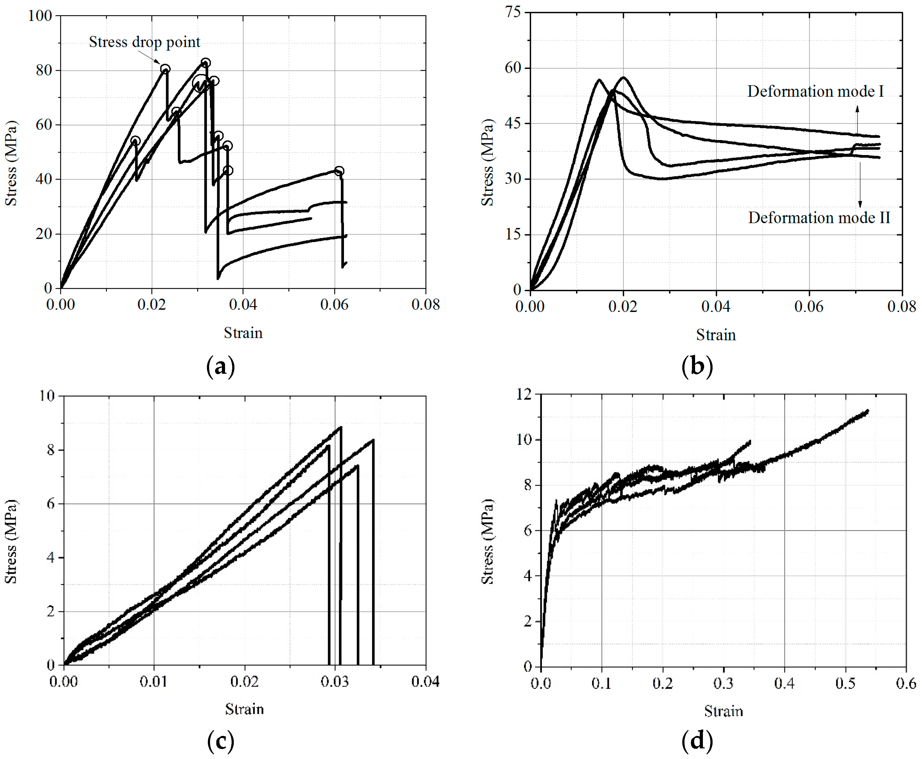
The stress–strain curves of wood under monotonic tension and compression are shown in Figure 6. It can be seen from Figure 6a that the ParG tensile stress–strain curves show different degrees of stress random drop phenomena with the increase in strain. Most of the stress drop phenomena in the specimens occur after the peak point. Although one specimen has a stress drop before the peak stress, the average peak strength of 75.8 MPa can still be reached in the subsequent loading process. It means that the stress drop before the peak value has little impact on its peak strength. Since no obvious damage was found on the surface of the specimen, the reason for the pre-peak stress drop is still unknown. When reaching peak strength, all the specimens produce different amplitudes of stress drop but are not completely destroyed. Instead, they continue to be tensioned based on the remaining effective fiber section until further random fracture of the wood fiber bundle occurs, resulting in the gradual destruction of wood.
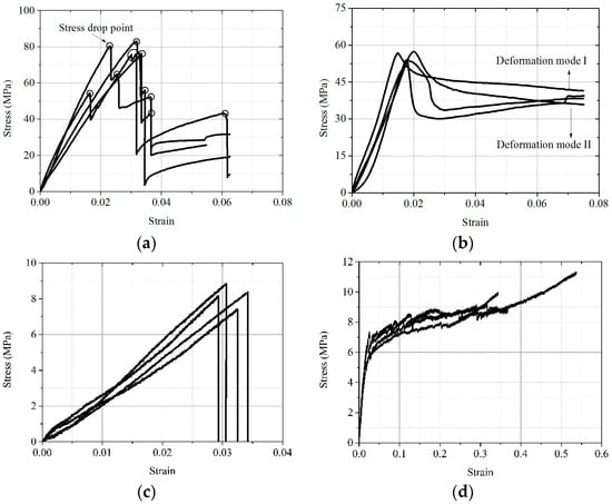
Figure 6.
Monotonic stress–strain curves. (a) Parallel-to-grain tension. (b) Parallel-to-grain compression. (c) Perpendicular-to-grain tension. (d) Perpendicular-to-grain compression.
It can be seen from the ParG stress–strain curves (Figure 6b) that the deformation process before the peak point is basically linear. After the peak point, there are two change laws corresponding to the buckling and shear failure modes, as previously described. The average values of the peak strengths of the two types of curves are 53.2 MPa and 58.8 MPa, respectively.
The monotonic PerG tensile and compressive stress–strain curves of wood are shown in Figure 6c,d. It can be seen from Figure 6c that the PerG tensile stress–strain curves of wood are generally approximately linear, and a relatively sudden brittle fracture occurs once reaching the peak point. The monotonic compression stress–strain curves under PerG loading show obvious three-stage deformation characteristics, namely linear elasticity, linear strain hardening, and secondary strain hardening. The average values of the peak strengths of the PerG tension and compression curves are 8.2 MPa and 6.7 MPa, respectively.
3.2.2. Cyclic Stress–Strain Curves
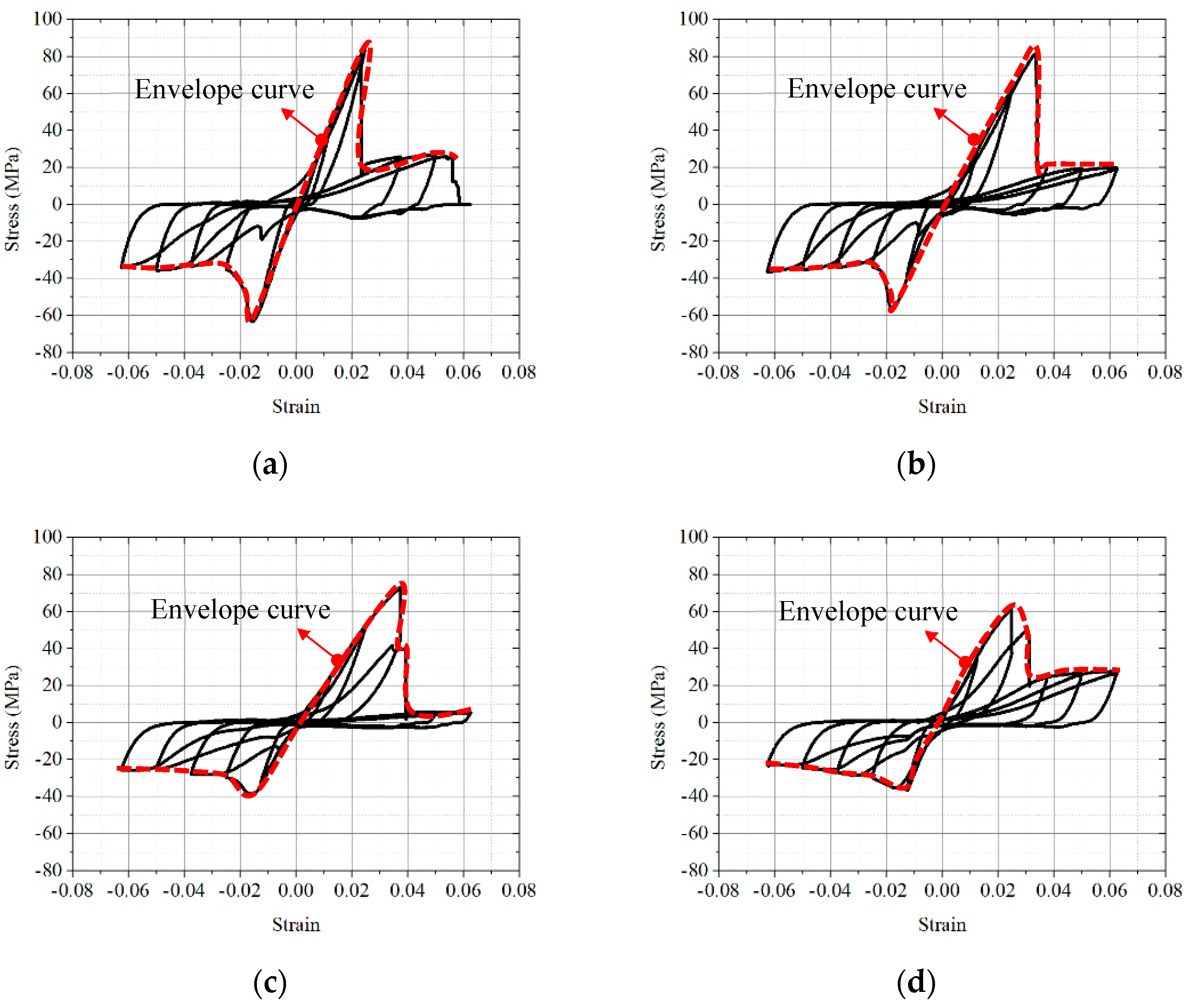
The stress–strain curves of wood under cyclic loading are shown in Figure 7. The tension part of the cyclic stress–strain curves is significantly asymmetric with the compression part. Generally, the ParG compression of wood shows similar ductile deformation to that under cyclic compression. Since the target stress of the reverse tension is set at 45 MPa, which is far less than the tensile strength of 60 MPa, all specimens are in the linear stress stage, and there is no random drop in tensile stress. Due to the influence of the ParG compression damage and the adverse effect of the tensile process on the compression damage, the stiffness under reverse loading has generally degraded.
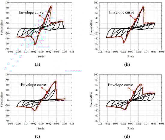
Figure 7.
ParG cyclic stress–strain curves of wood. (a) CS1-1. (b) CS1-2. (c) CS1-3. (d) CS1-4.
It can be seen from Figure 7 that the ParG cyclic stress–strain curves of wood consist of six parts, namely the tensile skeleton curve, the tensile unloading curve, the reverse compression curve after tensile unloading, the compression skeleton curve, the compression unloading curve, and the reverse tension curve after compression unloading.
The deformation characteristics of the skeleton curves under cyclic loading are similar to those under monotonic tension and compression. On the whole, the shapes of the unloading curves are very similar to each other, showing a downward convex trend to the right. However, there are generally different degrees of dispersion in each group of unloading curves at different unloading points. When unloading before the peak point, the discreteness is small. After the peak point, due to the stress drop phenomenon of different degrees, the unloading stiffness has a large discreteness. With the increase in strain at the unloading point, the discreteness is more significant. It can also be seen that the random drop in stress leads to the discreteness of the strain at the initial point of reverse compression (the strain when the tension unloading curve unloads to zero stress), which increases with the increase in the unloading point strain.
The cyclic stress–strain curves of wood under perpendicular-to-grain loading are shown in Figure 8. It can be seen that the general trend of the two types of cyclic curves at the compression side is similar to the corresponding cyclic compression situation, and the skeleton curve is similar to the corresponding uniaxial compression situation. Because of the influence of compression damage on the tensile side, when the strain at the compression unloading point is small, the reverse tensile curve shows an approximate linear change trend, which is similar to the change trend under monotonic loading. However, when strain at the compression unloading point is large, the nonlinear characteristics of the reverse tension curve are significant, showing a different trend from its monotonic case.
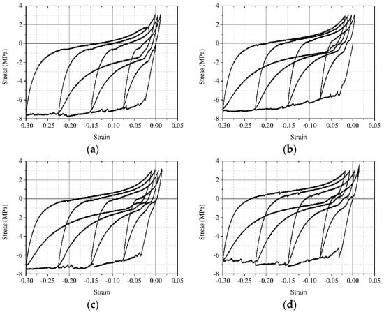
Figure 8.
PerG cyclic stress–strain curves of wood. (a) CR1-1. (b) CR1-2. (c) CR1-3. (d) CR1-4.
The PerG cyclic stress–strain curves of wood show significant asymmetry (see Figure 8). The overall stress–strain curve converges from the compression side to the tension side until the target tensile stress is reached. As the stress control scheme was adopted at the tensile side in the test, the stress–strain curve is unloaded from the compressive side and reaches the tensile target stress during the tensile process. The tensile strains corresponding to the target tensile stress that occur in individual specimens under different stress amplitudes are almost identical.
4. Constitutive Model of Wood
4.1. Monotonic Constitutive Model
4.1.1. Parallel-to-Grain Tension
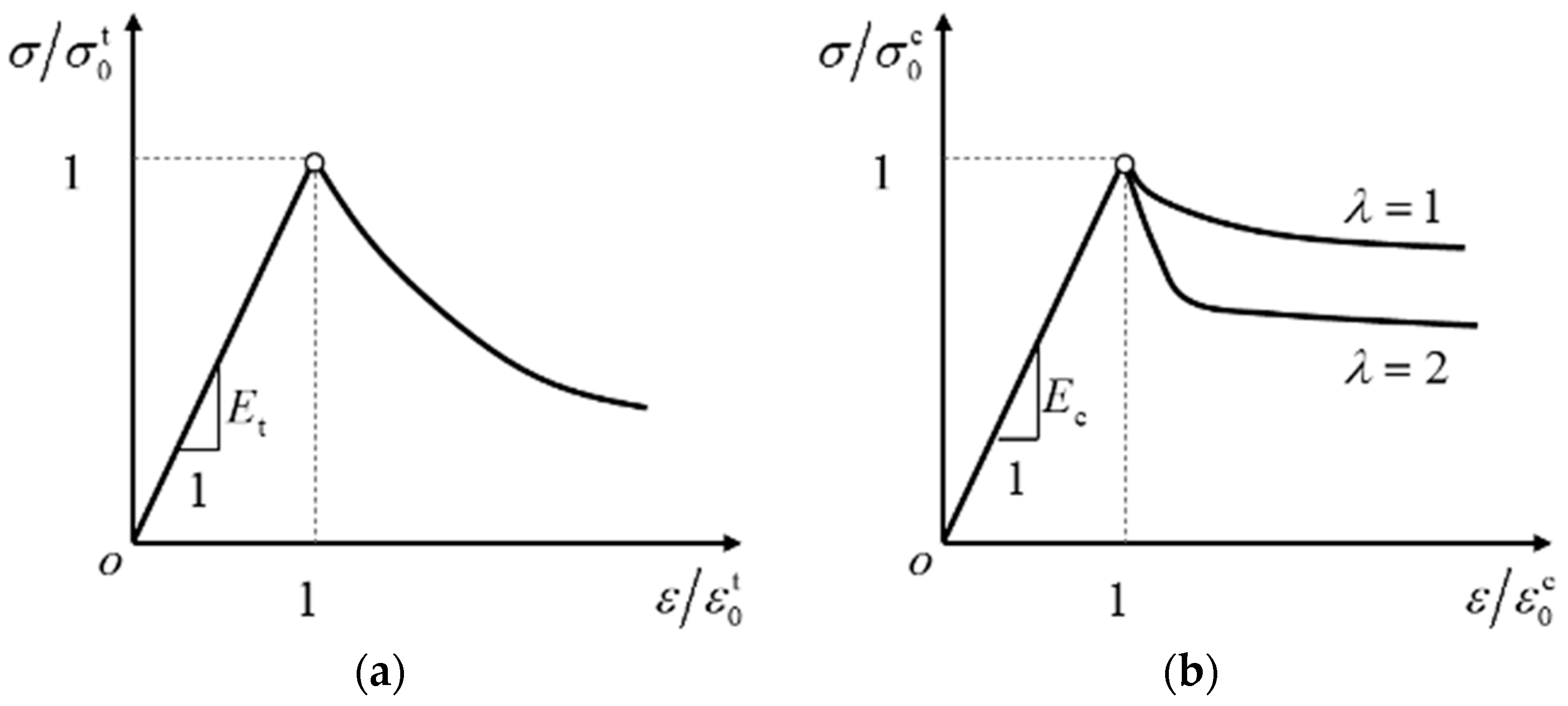
The monotonic tensile stress–strain curve of wood parallel to the grain shows approximately linear and random stress drop phenomena before and after the peak point, which can be described by a linear function and an exponential function before and after the peak point, respectively (see Figure 9a). The tensile stress–strain model of wood parallel to grain can be characterized by Equation (1).
where and represent the ParG tensile stress and strain, respectively; , , and represent the tensile modulus of elasticity, the peak tensile stress, and the peak tensile strain along the grain direction, respectively, with ; and , , and are dimensionless model coefficients that control the change in the tensile stress–strain curve of wood after the peak point. The average values of , , and are determined by experiment data to be 0.04, 211.1, and −2.3, respectively.

Figure 9.
Monotonic ParG constitutive model of wood. (a) Tension. (b) Compression.
4.1.2. Parallel-to-Grain Compression
The monotonic compression stress–strain curve of wood along the grain presents an approximate linear change trend before the peak point, and there are two bifurcation curves of compression and shear after the peak point, as shown in Figure 10b. The mathematical model is shown in Equation (2).
where , , and represent the elastic modulus, the peak compressive stress, and the peak compressive strain of wood in PerG compression, with ; and , , , and () are the ParG compression model coefficients, which control the change trend of the stress–strain curve after the peak point of the wood. The average values of parameters , , and are 0.7, −2.0, and 0.2, respectively; the average values of () are 3.39, −4.19, 2.19, −0.48, and 0.038; and is the control parameter of the wood compression failure mode along the wood grain and takes values 1 and 2 for compression and shear failure modes, respectively.
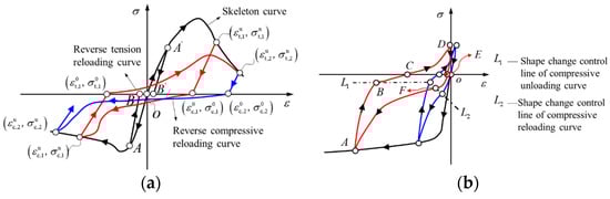
Figure 10.
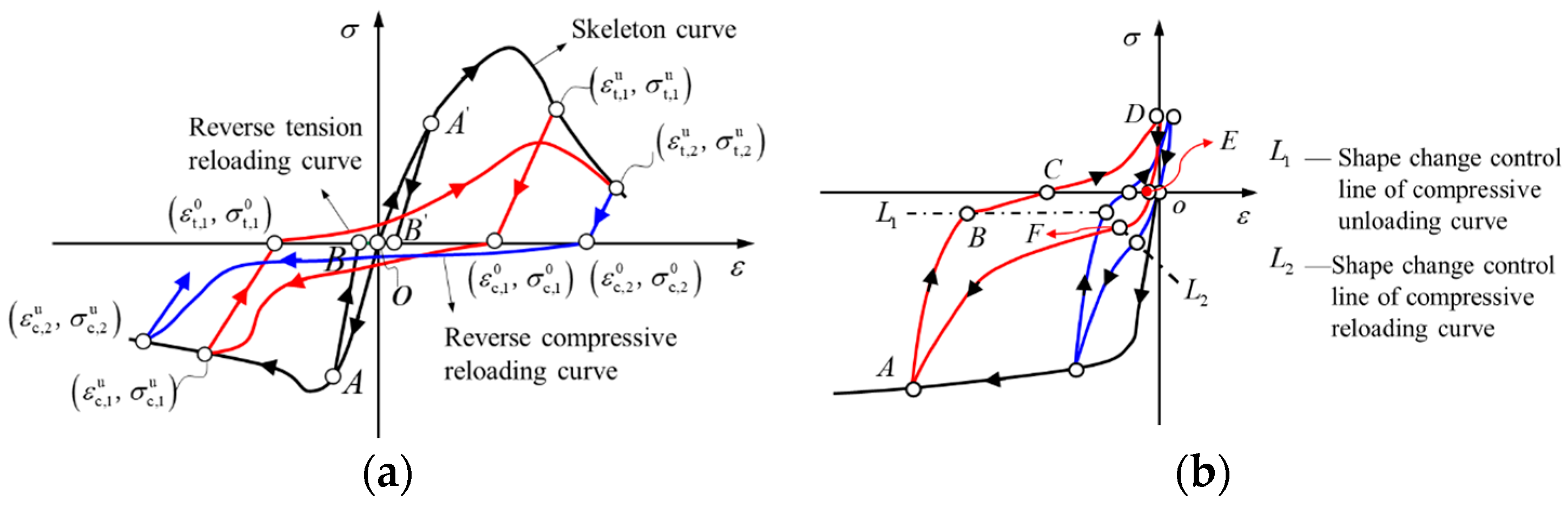
Schematic diagram of the hysteresis rules of wood under cyclic loading. (a) Parallel to grain. (b) Perpendicular to grain.
4.1.3. Perpendicular-to-Grain Constitutive Model
The perpendicular-to-grain monotonic constitutive model of wood includes the tensile model and the compression model. It can be seen from the test results that the monotonic tensile curves of wood in the radial direction are linear and can be characterized by a linear model, while the compression curve is nonlinear and can be approximately characterized by the bilinear model, as shown in Equation (3).
where is the correction coefficient of elastic modulus in the strain-hardening branch of wood after yielding on the compression side, and and are the ultimate strain in tension and the peak strain in compression in the transverse direction of the wood, respectively. The values of model parameters , , , , and are obtained by data fitting to be 260.4 MPa, 222.8 MPa, 0.04, 0.03, and −0.03, respectively.
4.2. Envelope Curve
The skeleton curves of wood under cyclic loading are composed of the tension side and compression side, which are similar to their corresponding uniaxial tension and compression curves, respectively. Therefore, the skeleton curve of wood can be obtained by modifying the uniaxial constitutive model.
4.2.1. Parallel-to-Grain Envelope Curve
The stress–strain skeleton curve of wood under parallel-to-grain cyclic loading is nearly the same as the monotonic curve, but the coordinates of the peak point are different. It means that the same expression for the uniaxial case can be used to describe the cyclic case, but the position of the peak point needs to be considered for model correction.
Based on the parallel-to-grain monotonic tension and monotonic compression stress–strain models expressed in Equations (1) and (2), the cyclic skeleton curve model can be obtained by adjusting the correlation coefficient through the modification of the peak point stress, the peak point strain, and the elastic modulus while keeping the model coefficients unchanged, as shown in Equation (4).
where , , , , , and are the parallel-to-grain peak strength, peak strain, and elastic modulus under cyclic loading, and , , , , , and are the model correction coefficients, whose values are shown in Table 2. Based on the monotonic model represented by Equations (1) and (2), the parallel-to-grain cyclic loading skeleton curve model can be obtained by substituting , , , , , and in Equation (4) for , , , , , and in Equations (1) and (2).
Table 2.
Model correction coefficients.
4.2.2. Perpendicular-to-Grain Skeleton Curve
The cyclic compression skeleton curve of the wood’s transverse grain can be directly described by the monotonic compression model, the second and third equations in Equation (3). The cyclic envelope curve model can be obtained by adjusting the correlation coefficient through the modification of the peak point stress, the peak point strain, the elastic modulus, and the correction coefficient of the hardening modulus while keeping the model coefficients unchanged, as shown in Equation (5).
where , , , and are the perpendicular-to-grain peak strength, peak strain, elastic modulus, and hardening modulus correction coefficients of wood under cyclic loading, respectively, and , , , and are the model correction coefficients, whose values are shown in Table 2. Based on the monotonic model represented by Equation (4), the perpendicular-to-grain cyclic skeleton curve model can be obtained by substituting , , , and in Equation (5) for , , , and in Equation (3).
4.3. Hysteresis Curve
4.3.1. Parallel-to-Grain Cyclic Model
Based on the results of the cyclic loading test of wood parallel to the grain, combined with its typical mechanical characteristics, the following hysteretic criteria for the stress–strain model are proposed:
- In the process of cyclic loading and unloading, both tension and compression unloading are expressed linearly by the corresponding unloading curve.
- After wood is unloaded under tension and compression, the reloading curve is described by the forward reloading model and the reverse reloading model, respectively.
- In the forward reloading model, the stress returns to the unloading starting point along the unloading curve and then continues to load according to the skeleton curve, while the reverse reloading model points to the skeleton curve in the opposite direction.
- At the unloading point, the strain and the corresponding irreversible deformation are small. The reverse reloading curve is usually assumed to continue loading along the reverse skeleton curve after loading along the strain axis (the stress is always 0) to the strain zero point.
- The tension skeleton curve implicitly considers the stress drop phenomenon and uses the smooth curve to express it, while the reverse tension reload curve explicitly describes the stress drop phenomenon.
The tensile and compressive unloading starting points of the cycle can be defined with (, ) and (, ). The tensile and compressive unloading completion points of the cycle can be defined with (, ) and (, ). The schematic diagram of the hysteresis rules of wood under cyclic loading is shown in Figure 10a.
- Compression and tension unloading models;
The unloading curve and forward reloading curve can be expressed as:
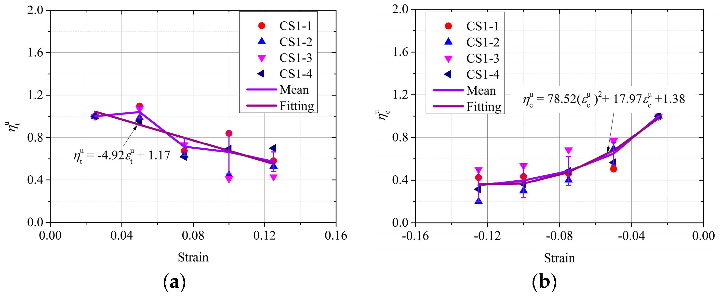
where and are cyclic tension and cyclic compression unloading moduli, respectively, whose values are determined by Equation (8) and Equation (9), respectively.
where is the unloading stiffness value corresponding to the unloading point strain of 0.0125, is the model parameter, and the relationship with the strain at the unloading point is shown in Figure 11a. is the unloading stiffness value corresponding to the unloading point strain of 0.0125, is the model parameter, and the relationship between the value and the strain at the unloading point is shown in Figure 11b.
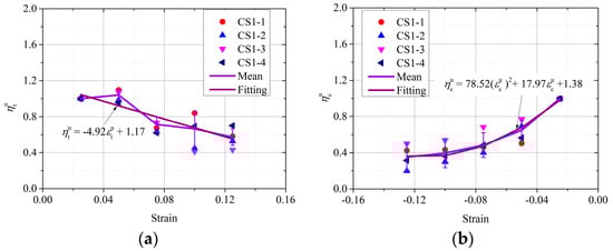
Figure 11.
Relation between model parameters and the strain of tensile unloading at the starting point. (a) . (b) .
- 2.
- Reverse compression reloading model;
According to the test results, when the strain at the unloading point in tension lies between 0.0125 and 0.025, the corresponding average strain at the starting point of reverse compression loading is 0.006 and 0.005, respectively. They are 4.8% and 8% of the total tensile strain of 0.0625 along the grain, respectively. Therefore, in the fourth quadrant, it can be described by loading along the strain axis to the coordinate origin and then continuing to load along the compression skeleton curve in the third quadrant.
When the strain is greater than 0.025, the reverse compression loading curve takes into account its part in the third and fourth quadrants and describes it according to the quintic polynomial until it is loaded onto the compression skeleton curve, as shown in Equation (9).
where are the model parameters whose values are related to the strain at the tension unloading point, as shown in Table 3.
Table 3.
Model parameters.
- 3.
- Reverse tension reloading model.
It can be seen from Figure 10a that when the unloading point of compression strain is greater than −0.025, the part of the curve in the second quadrant is very small. It can be approximately developed horizontally along the strain axis according to the stress and then loaded along the tensile skeleton curve after entering the first quadrant. When the stress drop occurs, it is necessary to analyze the stress drop position, stress drop amplitude, and continuous stress behavior of the drop and establish its stress–strain model through averaging. Without a stress drop, the shape and change trend of the stress–strain curves are similar through analysis, and the average stress–strain curve is established in three stages.
In the first stage, when the strain at the pressure unloading point exceeds −0.025 but has not reached −0.0375, a random stress drop generally occurs. The average value of a stress drop is 46.32 MPa, and the average strain at the stress drop point is 0.03. The complete reverse tensile stress–strain model can be defined as:
where is the reference stress, and its average value is −22.44 MPa; and are the model parameters with mean values of 30.02 and 35.40, respectively; is the initial point strain of reverse tension; and and are the stress and strain at the stress drop point, respectively.
In the second stage, when the strain at the compression unloading point is less than −0.0375 but greater than −0.1, part of the curve will extend to the skeleton curve after the stress drop, and then the unloading will occur. For this section of the tension and reloading curve, it is also necessary to carry out the work in sections, and it is considered necessary to introduce the parameter (stress drop switch) to distinguish stress drop from stress drop. The tensile reloading curve considering the effect of stress drop () is characterized by Equation (11), but the values of relevant parameters are different. The tensile reloading curve without considering the effect of stress drop () is characterized by Part 1 of Equation (11), that is:
- When (considering stress drop), Equation (10) is adopted, and the relevant parameters are a drop point strain of 0.038 and a drop stress of 27.3 MPa. The values of the other parameters are = −8.1 MPa, = 11.7, and = 32.6.
- When (without considering the stress drop), the first formula in Equation (10) is used, and the relevant parameters are = −10.7 MPa, = 15.8, and = 32.0.
- In the third stage, when the strain at the compression unloading point is less than −0.05, the reload curve is characterized by the first formula of Equation (10), and the corresponding parameter values are = −4.52 MPa, = 7.14 MPa, and = 81.34.
4.3.2. Perpendicular-to-Grain Cyclic Model
The perpendicular-to-grain cyclic constitutive model of wood includes the cyclic compression skeleton curve model and the cyclic hysteretic rule.
The skeleton curve model of wood is adopted according to uniaxial compression. The hysteretic rule of wood under cyclic loading is shown in Figure 10b. The mathematical description method of the cyclic loading process is established in two steps. First, the corresponding relationship between the critical control points of the hysteretic curve and the strain of the compression unloading control points is established. Second, the control equations for each section of the hysteretic curve are established.
- Strain analysis of critical control points;
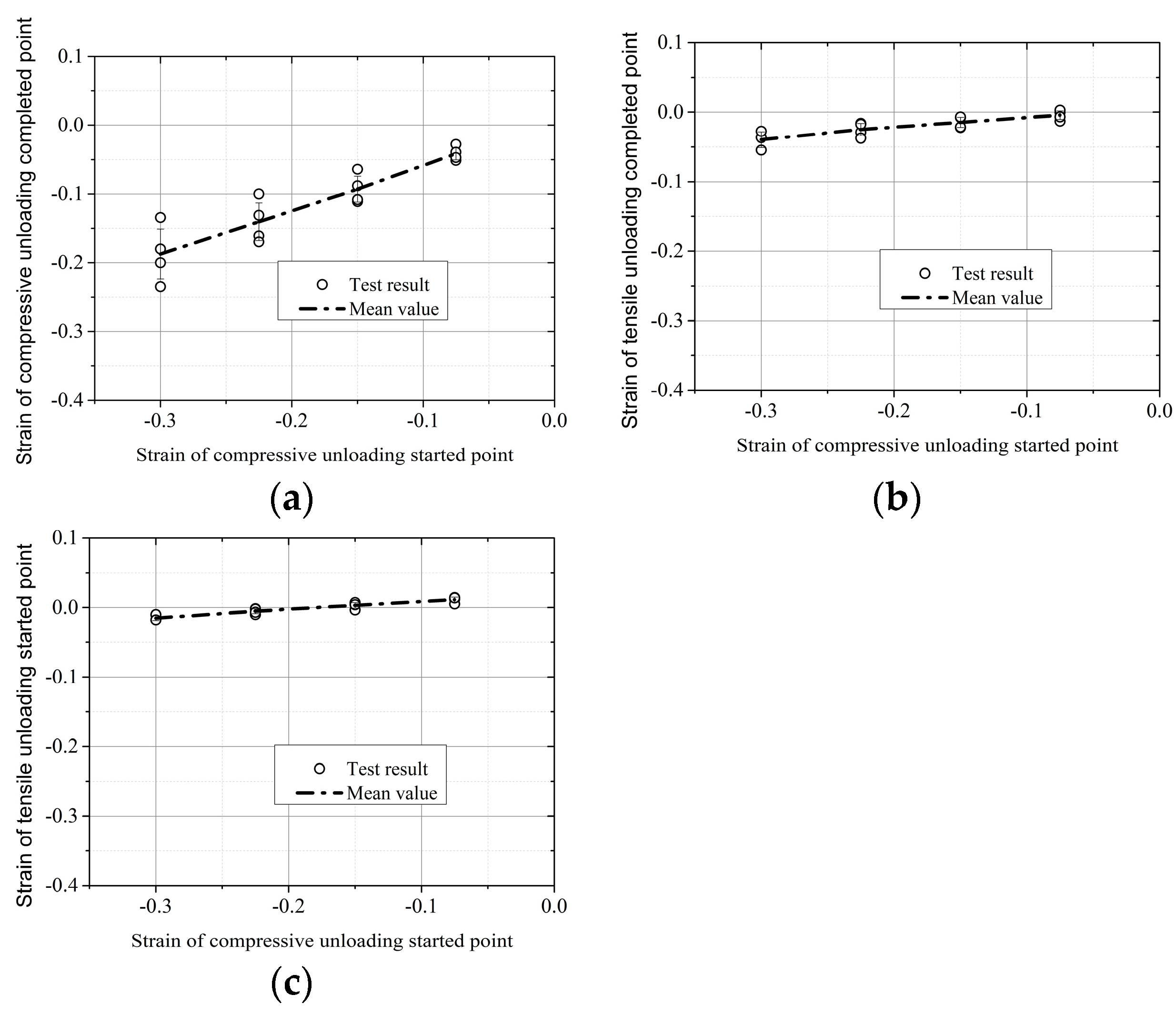
There are four key control points on the cyclic tension and compression path of wood cross grain, namely points A (, ), C (, 0), D (, ), and E (, 0). The strain and stress at the starting point A of compression unloading are determined by the skeleton curves of the cyclic tension and compression curves, respectively. The stress at points C and E is always 0, but it is necessary to determine its corresponding strain and relationship with the strain at the beginning of compression unloading. The stress at tension unloading point D remains constant at 3 MPa, but it is also necessary to determine the relationship between its strain and the strain at the beginning of compression unloading, as shown in Equation (12) and Figure 12.
where , , , , , and are model coefficients, the values of which are 0.554, 4.59 × 10⁻³, 0.142, 9.64 × 10⁻³, 0.038, and 3.05 × 10⁻³, respectively.
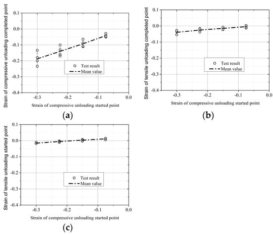
Figure 12.
Relation between the critical strain of the cyclic curves and the strain of compressive unloading at the starting point. (a) . (b) . (c) .
- 2.
- Compression unloading model;
The cyclic stress–strain hysteretic curve of wood includes the compression unloading curve and the reverse tension curve after compression unloading, as well as the compression unloading curve and reverse compression curve after tension unloading.
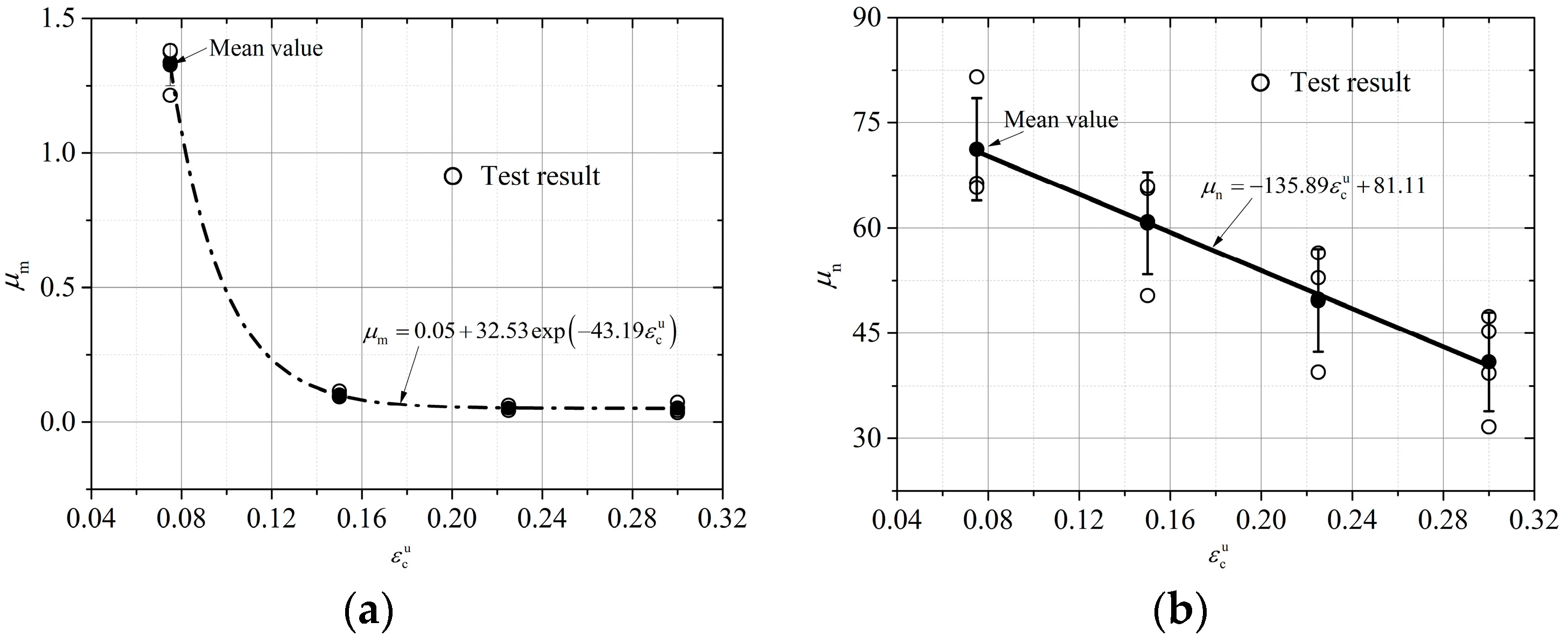
The shape of the compressive unloading curves corresponding to different unloading starting points is similar, but the residual deformation after unloading is quite different. Therefore, the same mathematical expression can be used to describe the perpendicular-to-grain compressive unloading curves of wood, expressed by a cubic polynomial in Equations (12)–(14).
where A and B are model parameters, and their expressions can be determined by fitting test data, and then the parameters , , , , and can be determined as 0.05, 32.53, −43.19, −135.89, and 81.11, respectively. The fitting results for parameters A and B are shown in Figure 13.

Figure 13.
Compression unloading stress–strain model parameters. (a) Parameter . (b) Parameter .
- 3.
- Reverse tensile stress–strain model;
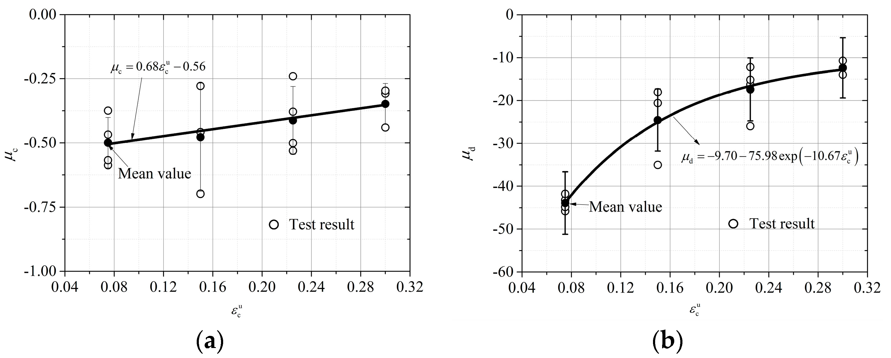
The reverse perpendicular-to-grain tensile stress–strain curves of wood specimens after compression unloading are shown in Figure 11b. It can be seen that since the two types of specimens have different degrees of residual strain after compression and unloading, the overall shape of the stress–strain curve under further tension is similar and can be described by Equation (16).
where and are model parameters whose correlation with the strain at the compression unloading starting point is shown in Equations (17) and (18) and Figure 14.
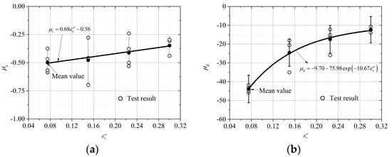
Figure 14.
Tensile stress–strain model parameters. (a) Parameter . (b) Parameter .
- 4.
- Tensile unloading stress–strain model;
The perpendicular-to-grain tensile unloading stress–strain curves of wood are shown in Figure 10b. It can be seen that there are different degrees of residual strain after unloading. The stress–strain curves can be approximately described by linear expressions, as shown in Equations (19) and (20).
where is the adjustment coefficient considering the jumping of the fitting curve at key numerical points. When is 0.075, 0.15, 0.225, and 0.3, the values of are 2, 1.842, 1.644, and 1.715, respectively, and the rest are determined by linear difference.
- 5.
- Reverse compressive stress–strain model.
The reverse perpendicular-to-grain compression curve after tension unloading in the cyclic stress–strain hysteretic curve is shown in Figure 10b. It can be seen that the overall shape of the curves has many similarities, while the reverse compression point deformation is different. The stress–strain curves can be described by Equation (21).
where M, N, K, and b are model parameters, and the correlation between them and the strain at the compression unloading point is shown in Equations (22) and (23).
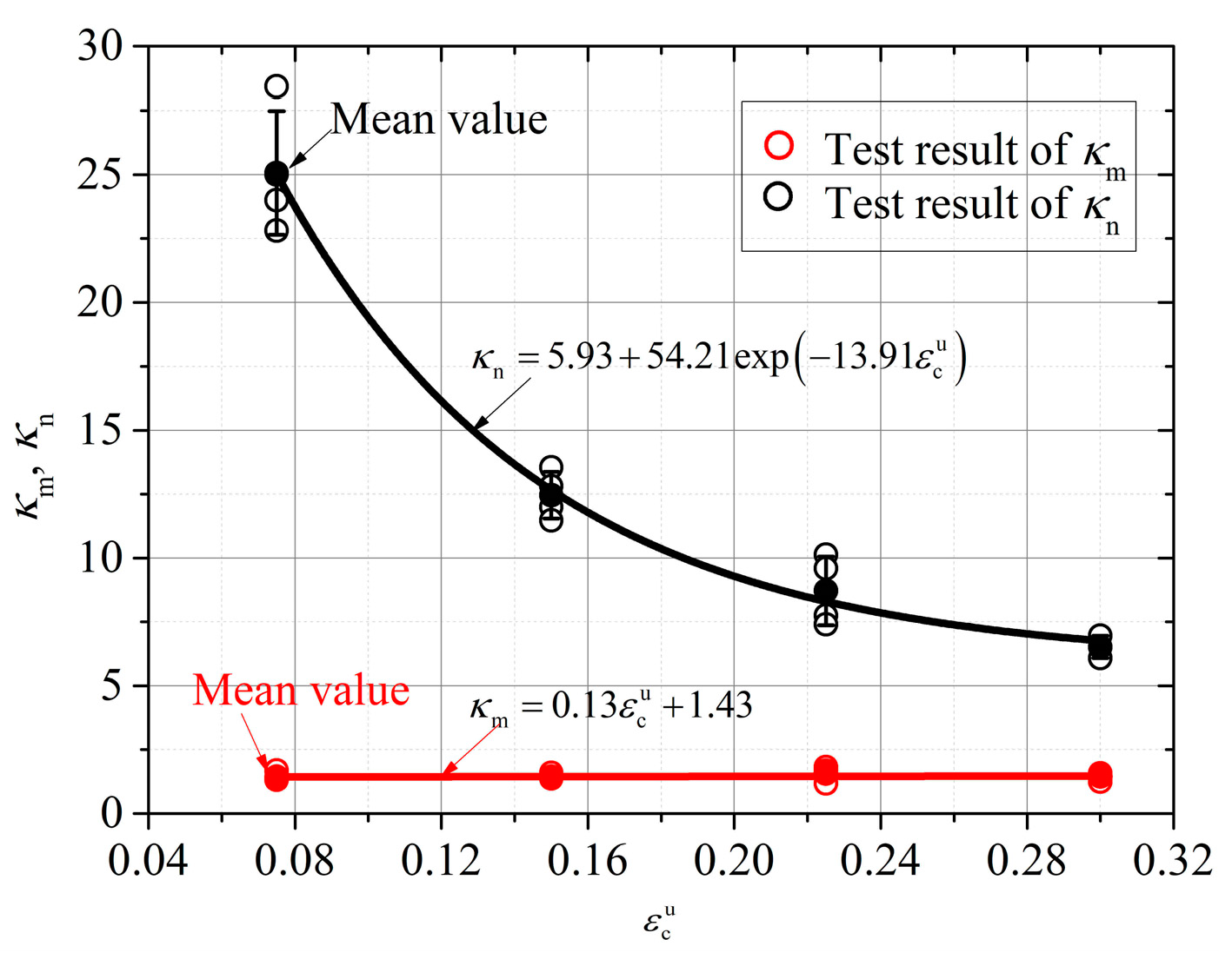
where the fitting results of parameters and are shown in Figure 15.
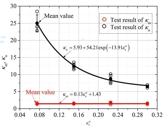
Figure 15.
Model parameters and .
5. Verification of the Constitutive Model
In order to verify the correctness of the established constitutive model of wood under the action of cyclic loading, the proposed model and relevant parameters in this paper are used to simulate the monotonic and cyclic loading processes of wood perpendicular and parallel to the grain.
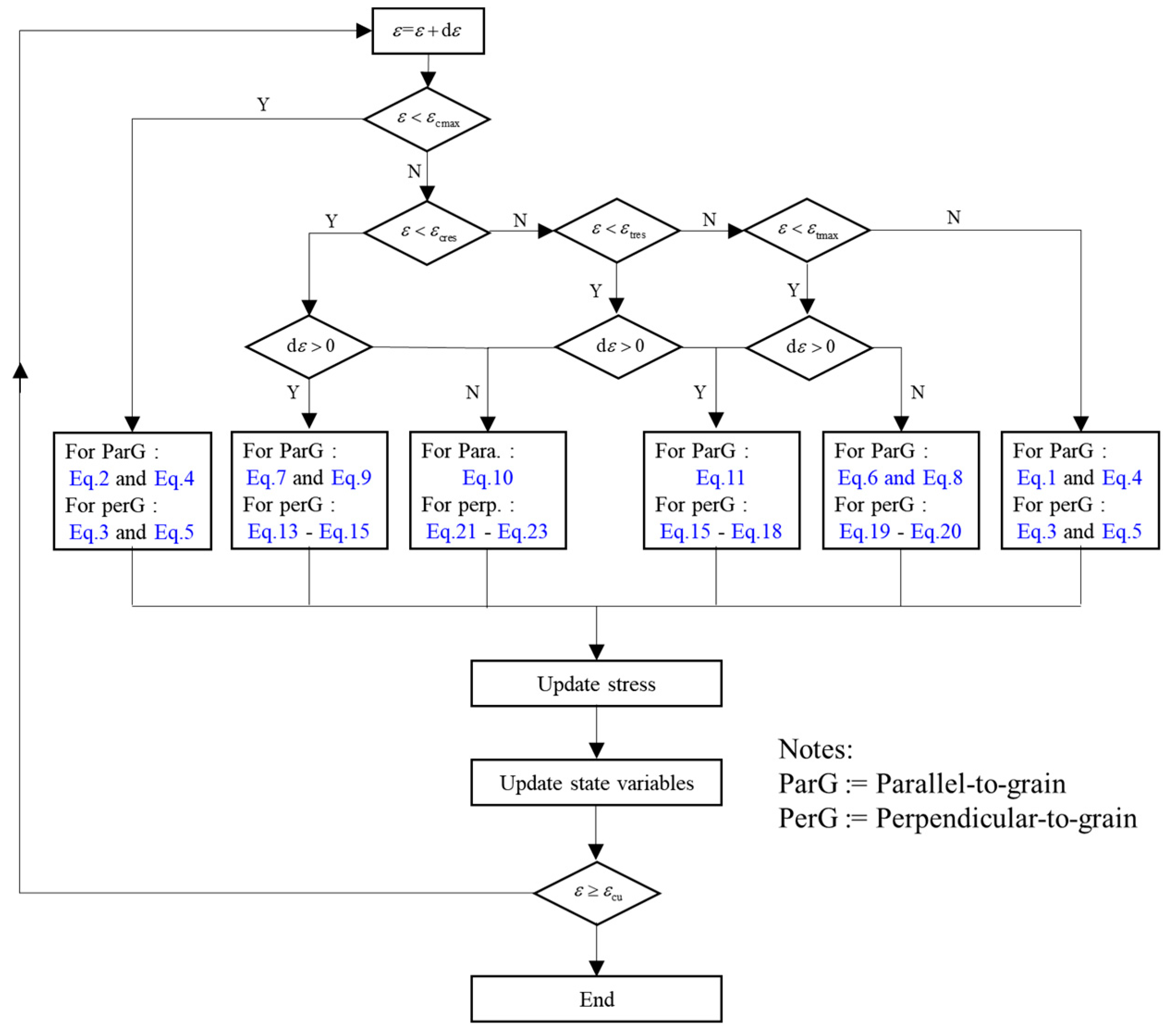
The calculation algorithm is shown in Figure 16. The aim was to update the stress according to the proposed cyclic constitutive model of wood parallel to the grain and perpendicular to the grain. The algorithm is driven by the strain increment, . The material parameters included in the proposed constitutive model were adopted. Four state variables were used to indicate the loading history, namely the maximum compressive (tensile) strain, (), and the residual compressive (tensile) strain, (), respectively. The loading and unloading criteria were indicated by , where means a compressive unloading or a tensile loading process and means a compressive loading or a tensile unloading process. The loading process will stop once the ParG and PerG compressive strains reach the ultimate value .
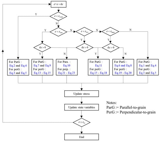
Figure 16.
Stress update algorithm.
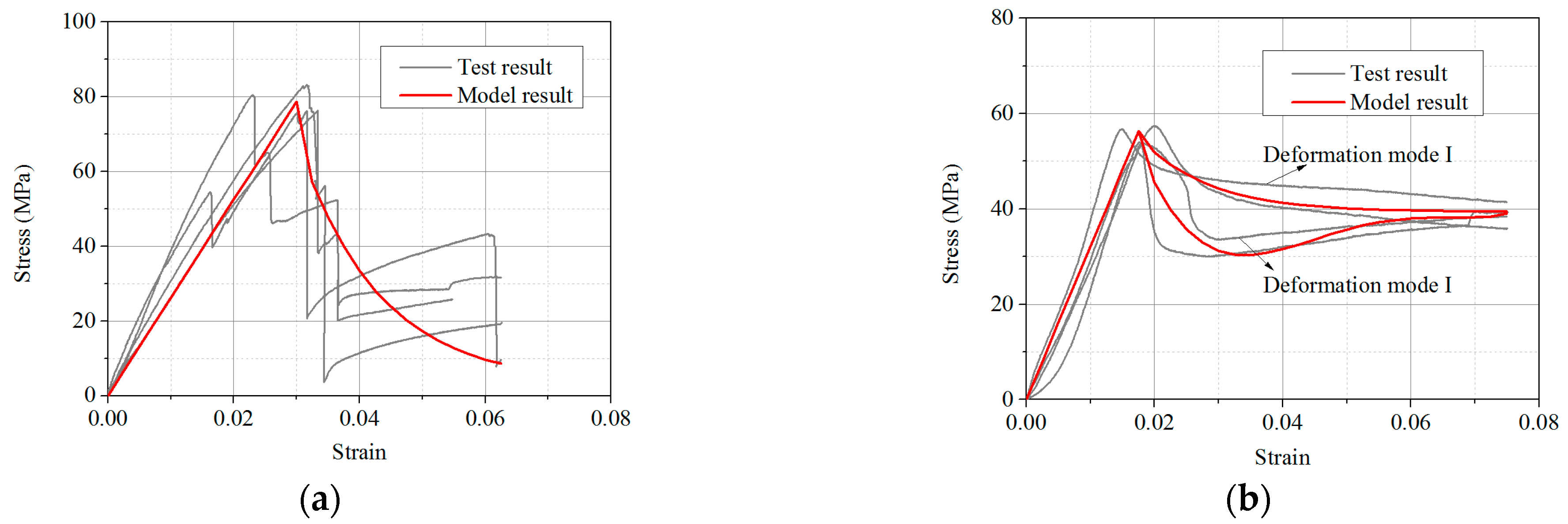
The model calculation results are compared with the tested stress–strain curves and shown in Figure 17. It can be seen that the monotonic tension and cyclic loading simulation curves are in good agreement with the test curves, verifying the correctness of the proposed constitutive model.
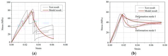
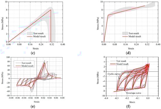
Figure 17.
Comparisons between test and model results. (a) Monotonic tension parallel to grain. (b) Monotonic tension perpendicular to grain. (c) Monotonic tension perpendicular to grain. (d) Monotonic compression perpendicular to grain. (e) Cyclic tension and compression parallel to grain. (f) Cyclic tension and compression perpendicular to grain.
6. Conclusions
Through the parallel-/perpendicular-to-grain cyclic loading test of the dog-bone specimens of the wood, the deformation mode, damage characteristics, and change rule were analyzed. The constitutive model that can comprehensively describe the cyclic loading behavior of the wood was established. The main conclusions are as follows:
- The main stress characteristics of monotonous and cyclic tension along the grain of wood are random fractures in different positions and different quantities of wood fibers after the peak point. The random drop in stress and the continuous loading mechanism based on the remaining effective section of wood until the specimen was completely broken were observed. In the process of cyclic tension, the loading and unloading of wood is coupled with a random drop in stress.
- There are two failure modes of wood observed under parallel-to-grain cyclic compression, namely buckling and shear. The stress–strain curve with the former failure characteristic shows that the stress after the peak point decreases smoothly and slowly with the increase in load, and the specimen has two damage bands. The stress–strain curve of the latter shows that the stress decreases suddenly and then rises slowly, and there is one kinking and torsion damage zone in the specimen.
- The complete stress–strain curve of wood under perpendicular-to-grain cyclic loading is significantly asymmetrical and converges from the compression side to the tension side. The compression unloading curve shows significant nonlinear stress characteristics, and irreversible deformation and unloading stiffness degradation are evident. There is an inflection point in the reverse compression stress–strain curve after unloading to zero under tension, which changes from convex to concave, and the stiffness degrades.
- Based on the test results of wood under parallel- and perpendicular-to-grain cyclic loading, the stress–strain model that can consider the degradation of cyclic compression unloading stiffness and the change in reverse compression (tension) stiffness after tension (compression) unloading is established. The model results are in good agreement with the test results.
- Although the proposed constructed constitutive model is able to describe the complex mechanical performance of wood in both the longitudinal and transverse directions under uniaxial and cyclic loading, there are still two aspects that need to be improved in the future. Firstly, the revelation of the damage mechanism of wood under different loading cases needs to be investigated. The second issue is to describe the hysteresis behavior of wood within the framework of damage mechanics and implement it into ABAQUS 6.14 software to provide support for nonlinear analysis of timber components and structures.
Author Contributions
Conceptualization, Q.X. and L.Z.; methodology, L.Z.; software, Y.H.; validation, Q.X., Y.H. and Y.W. (Yingjin Wang); formal analysis, L.Z.; investigation, L.Z.; resources, L.Z.; data curation, Y.H.; writing—original draft preparation, L.Z.; writing—review and editing, L.Z. and Y.W. (Yajie Wu); visualization, L.Z.; supervision, Q.X.; project administration, Q.X.; funding acquisition, Q.X. All authors have read and agreed to the published version of the manuscript.
Funding
This research was funded by the National Natural Science Foundation of China (Grant No. 52178303), the key R&D Program in Shaanxi Province (2023-GHZD-03), the Shaanxi Natural Science Basic Research Program (No. 2018JC-025, 2021JC-44 and 2023JC-QN-0409), and the 2023 R&D Program from XAUAT Engineering Technology Co., LTD (No. XAJD-YF23N015).
Data Availability Statement
Data will be available upon request.
Conflicts of Interest
The authors declare no conflict of interest.
References
- Xie, Q.F.; Zhang, L.P.; Li, S.; Zhou, W.J.; Wang, L. Cyclic behavior of Chinese ancient wooden frame with mortise–tenon joints: Friction constitutive model and finite element modelling. J. Wood Sci. 2018, 64, 40–51. [Google Scholar] [CrossRef]
- Xie, Q.F.; Zhang, L.P.; Miao, Z.; Zhou, W.J. Lateral behavior of traditional Chinese timber frames strengthened with shape memory alloy: Experiments and analytical model. J. Struct. Eng. 2020, 146, 04020083. [Google Scholar] [CrossRef]
- Hua, Y.W.; Chun, Q. Influence of Pu-zuo on progressive collapse behavior of ancient southern Chinese timber buildings built in the Song and Yuan dynasties: Experimental Research. Eng. Fail. Anal. 2022, 137, 137. [Google Scholar] [CrossRef]
- Babanc, M.B. Examination of the failures and determination of intervention methods for historical Ottoman traditional timber houses in the Cumalkzk Village, Bursa-Turkey. Eng. Fail. Anal. 2013, 35, 470–479. [Google Scholar]
- He, J.X.; Wang, J. Theoretical model and finite element analysis for restoring moment at column foot during rocking. J. Wood Sci. 2018, 64, 97–111. [Google Scholar] [CrossRef]
- Vazquez, C.; Gonçalves, R.; Bertoldo, C.; Baño, V.; Vega, A.; Crespo, J.; Guaita, M. Determination of the mechanical properties of castanea sativa mill. using ultrasonic wave propagation and comparison with static compression and bending methods. Wood Sci. Technol. 2015, 49, 607–622. [Google Scholar] [CrossRef]
- Bachtiar, E.V.; Sanabria, S.J.; Mittig, J.P.; Niemz, P. Moisture-dependent elastic characteristics of walnut and cherry wood by means of mechanical and ultrasonic test incorporating three different ultrasound data evaluation techniques. Wood Sci. Technol. 2017, 51, 47–67. [Google Scholar] [CrossRef]
- Jiang, J.L.; Bachtiar, E.V.; Liu, J.X.; Niemz, P. Comparison of moisture-dependent orthotropic young’s moduli of chinese fir wood determined by ultrasonic wave method and static compression or tension tests. Eur. J. Wood Wood Prod. 2018, 76, 953–964. [Google Scholar] [CrossRef]
- Oudjene, M.; Khelifa, M. Finite element modeling of wooden structures at large deformations and brittle failure prediction. Mater. Des. 2009, 30, 4081–4087. [Google Scholar] [CrossRef]
- Guan, Z.W.; Zhu, E.C. Finite element modelling of anisotropic elasto-plastic timber composite beams with openings. Eng. Struct. 2009, 31, 394–403. [Google Scholar] [CrossRef]
- Chen, Z.Y.; Zhu, E.C.; Pan, J.L. Numerical simulation of mechanical behaviour of wood under complex stress. Chin. J. Comput. Mech. 2011, 28, 629–634. [Google Scholar]
- Yang, N.; Zhang, L.; Qin, S.J. A nonlinear constitutive model for characterizing wood under compressive load and its test verification. China Civ. Eng. J. 2017, 50, 80–88. [Google Scholar]
- Sandhaas, C. Mechanical Behaviour of Timber Joints with Slotted-in Steel Plates. Ph.D. Thesis, Technische Universiteit, Delft, The Netherlands, 2012. [Google Scholar]
- Gharib, M.; Hassanieh, A.; Valipour, H.R.; Bradford, M.A. Three-dimensional constitutive modelling of arbitrarily orientated timber based on continuum damage mechanics. Finite Elem. Anal. Des. 2017, 135, 79–90. [Google Scholar] [CrossRef]
- Eslami, H.; Jayasinghe, L.B.; Waldmann, D. Nonlinear three-dimensional anisotropic material model for failure analysis of timber. Eng. Fail. Anal. 2021, 130, 105764. [Google Scholar] [CrossRef]
- Arruda, M.R.T.; Trombini, M.; Pagani, A. Implicit to Explicit Algorithm for ABAQUS Standard User-Subroutine UMAT for a 3D Hashin-Based Orthotropic Damage Model. Appl. Sci. 2023, 13, 1155. [Google Scholar] [CrossRef]
- Sirumbalzapata, L.F.; Málagachuquitaype, C.; Elghazouli, A.Y. A three-dimensional plasticity-damage constitutive model for timber under cyclic loads. Comput. Struct. 2017, 195, 47–63. [Google Scholar] [CrossRef]
- Wang, M.Q.; Song, X.B.; Gu, X.L. Three-Dimensional Combined Elastic-Plastic and Damage Model for Nonlinear Analysis of Wood. J. Struct. Eng. 2018, 144, 04018103. [Google Scholar] [CrossRef]
- Benvenuti, E.; Orlando, N.; Gebhardt, C.; Kaliske, M. An orthotropic multi-surface damage-plasticity FE-formulation for wood: Part I—Constitutive model. Comput. Struct. 2020, 240, 106350. [Google Scholar] [CrossRef]
- Zhang, L.P.; Xie, Q.F.; Zhang, B.Z.; Wang, L.; Yao, J.T. Three-dimensional elastic-plastic damage constitutive model of wood. Holzforschung 2021, 75, 526–544. [Google Scholar] [CrossRef]
- Chen, Z.Y.; Ni, C.; Dagenais, C.; Kuan, S. A temperature-dependent plastic-damage constitutive model, woodst, for numerical simulation of wood-based materials and connections. J. Struct. Eng. 2019, 146, 04019225. [Google Scholar] [CrossRef]
- Jiang, S.F.; Qiao, Z.H.; Wu, M.H.; Ouyang, Q. Study on wooden constitutive model considering long-term effects of environment and load. J. Build. Struct. 2021, 42, 160–168. [Google Scholar]
- Zhang, L.P.; Xie, Q.F.; Liu, Y.J.; Zhang, B.Z.; Wu, Y.J. Elastic-plastic damage constitutive model and numerical implementation for timber considering seismic strain rate effects. Chin. Civ. Eng. J. 2022, 56, 22–31. [Google Scholar]
- Yu, T.; Khaloian, A.; Jan-Willem, V.D.K. An improved model for the time-dependent material response of wood under mechanical loading and varying humidity conditions. Eng. Struct. 2022, 259, 114116. [Google Scholar] [CrossRef]
- Xie, Q.F.; Zhang, L.P.; Wang, L.; Wu, F.F. Research on radial stress-strain model of wood under repeated compressive loading. J. Hunan Univ. Nat. Sci. 2018, 45, 55–61. [Google Scholar]
- Edzang, A.C.E.; Nziengui, C.F.P.; Ango, S.E.; Ikogou, S.; Pitti, R.M. Comparative studies of three tropical wood species under compressive cyclic loading and moisture content changes. Wood Mater. Sci. Eng. 2021, 16, 196–203. [Google Scholar] [CrossRef]
- Zhang, C.H.; Liao, H.J.; Qian, C.Y.; Li, H.Z.; Song, L.; Zheng, J.G. Tensile-compressive fatigue experiment of wood of ancient building. Eng. Mech. 2016, 33, 201–206. [Google Scholar]
- GB/T-1927.5. Test Method for Physical and Mechanical Properties of Small Clear Wood Specimens—Part 5: Determination of Density; China Architecture & Building Press: Beijing, China, 2021. (In Chinese)
- GB/T 1927.4. Test Method for Physical and Mechanical Properties of Small Clear Wood Specimens—Part 4: Determination of Moisture Content; China Architecture & Building Press: Beijing, China, 2021. (In Chinese)
- GB/T 1927.3. Test Method for Physical and Mechanical Properties of Small Clear Wood Specimens—Part 3: Determination of the Growth Rings Width and Latewood Rate of Wood; China Architecture & Building Press: Beijing, China, 2021. (In Chinese)
- GB/T 1935. Method of Testing in Compressive Strength Parallel to Grain of Wood; China Architecture & Building Press: Beijing, China, 2009. (In Chinese)
- GB/T 1938. Method of Testing in Tensile Strength Parallel to Grain of Wood; China Architecture & Building Press: Beijing, China, 2009. (In Chinese)
- GB/T 1939. Method of Testing in Compressive Strength Perpendicular to Grain of Wood; China Architecture & Building Press: Beijing, China, 2009. (In Chinese)
- GB/T 1927.5. Test Method for Physical and Mechanical Properties of Small Clear Wood Specimens—Part 2: Sampling Methods and General Requirements; China Architecture & Building Press: Beijing, China, 2021. (In Chinese)
- GB 50005. Standard for Design of Timber Structures; China Architecture & Building Press: Beijing, China, 2017. (In Chinese)


Disclaimer/Publisher’s Note: The statements, opinions and data contained in all publications are solely those of the individual author(s) and contributor(s) and not of MDPI and/or the editor(s). MDPI and/or the editor(s) disclaim responsibility for any injury to people or property resulting from any ideas, methods, instructions or products referred to in the content. |
© 2023 by the authors. Licensee MDPI, Basel, Switzerland. This article is an open access article distributed under the terms and conditions of the Creative Commons Attribution (CC BY) license (https://creativecommons.org/licenses/by/4.0/).