Investigating the Effects of Parameter Tuning on Machine Learning for Occupant Behavior Analysis in Japanese Residential Buildings

Abstract

Global warming is currently progressing worldwide, and it is important to control greenhouse gas emissions from the perspective of adaptation and mitigation. Occupant behavior is highly individualized and must be analyzed to accurately determine a building’s energy consumption. However, most of the resident behavior models in existing studies are based on statistical methods, and their accuracy in parameter tuning has not been examined. The accuracy of heating behavior prediction has been studied using three different methods: logistic regression, support vector machine (SVM), and deep neural network (DNN). The generalization ability of the support vector machine and the deep neural network was improved by parameter tuning. The parameter tuning of the SVM showed that the values of C and gamma affected the prediction accuracy. The prediction accuracy improved by approximately 11.9%, confirming the effectiveness of parameter tuning on the SVM. The parameter tuning of the DNN showed that the values of the layer and neuron affected prediction accuracy. Although parameter tuning also improved the prediction accuracy of the DNN, the rate of increase was lower than that of the SVM.

1. Introduction

The building sector is currently responsible for more than 40% of global energy consumption and more than 30% of greenhouse gas (GHG) emissions [1]. The Intergovernmental Panel on Climate Change (IPCC)’s Sixth Assessment Report [2] states that anthropogenic GHG emissions increased approximately 1.6 times between 1990 and 2019, and the global average temperature increased by approximately 1.1 °C between 1850 and 2020. Achieving carbon neutrality is necessary to achieve a sustainable society, and it is imperative to address mitigation measures to reduce GHG emissions and adaptation measures to limit the damage that cannot be avoided by implementing mitigation measures alone [3].

Mitigation measures in the building sector include the use of more efficient buildings and renewable energy. To implement mitigation measures, understanding the indoor thermal environment and energy use by combining empirical measurements and computational simulations holds significant importance. However, the predictions obtained from current simulations differ from actual measurements [4,5]. One reason for the difference between the predicted and measured values is that the simulations do not reflect occupants’ behaviors in adapting to the indoor environment. Occupant behaviors include opening and closing windows, using heating and cooling equipment, and adjusting clothing. It is known that occupants’ behaviors change with thermal stress and can be considered in the simulations as a schedule model. For this purpose, it is necessary to develop a predictive model for occupant behavior based on observable variables. The analysis of occupant behavior is an adaptation measure to climate change.

In recent years, advances in hardware and information technology (IT) have brought machine learning to the forefront of data prediction. Machine learning is a technique for developing algorithms that make predictions by having the machine read data and iteratively learn to find hidden patterns [6]. Machine learning has been applied in various fields, including medicine, finance, agriculture, and commerce. Machine learning has also been used in the building sector, mainly to predict the energy consumption of buildings. However, there have been no studies in which machine learning has been used to predict occupant behavior. Machine learning techniques are also expected to improve prediction accuracy in the area of occupant behavior.

The effect of occupant behavior on energy consumption has been studied in a variety of buildings. Nicol and Humphreys [7] studied occupant behavior across Europe, including Pakistan and the United Kingdom, and presented a probabilistic approach to thermal comfort. Clevenger et al. [8] showed that occupant behavior affects annual energy consumption in residential and commercial buildings. Ioannou and Itard [9] showed that occupant behavior factors have a greater impact on heating energy consumption than building factors. Sun and Hong [10] demonstrated that a set of five indicators capturing occupant behavior, encompassing lighting, plug load, comfort, HVAC control, and window control, can reduce energy consumption by up to 22.9% alone and 41.0% in combination, respectively. Zhuang et al. [11] presented a data-driven predictive control method with time-series forecasting (TSF) and reinforcement learning (RL) to examine various sensor metadata for HVAC system optimization. The optimal TSF models were integrated with a Soft Actor-Critic RL agent to analyze sensor metadata and optimize HVAC operations, achieving 17.4% energy savings and 16.9% thermal comfort improvement in the surrogate environment. Zou et al. [12] presented Win Light, a novel occupancy-driven lighting control system that aims to reduce energy consumption while simultaneously preserving the lighting comfort of occupants. The experimental results demonstrated that Win Light achieved 93.09% and 80.27% energy savings compared to static-scheduling lighting control schemes and PIR sensor-based lighting control schemes while guaranteeing the personalized lighting comfort of each occupant. Duygu Tekler et al. [13] proposed Plug-Mate, a novel IoT-based occupancy-driven plug-load management system that reduces plug-load energy consumption and user burden through intelligent plug-load automation. Duygu Tekler et al. [14] proposed a hybrid active learning framework to reduce data collection costs for developing data-efficient and robust personal comfort models that can predict users’ thermal comfort and air-movement preferences. Andre et al. [15] reviewed recent publications on PCS to understand what has not yet been discussed on this topic. Wang and Greenberg [16] studied the effects of opening and closing windows on occupant behavior and showed that in summer months in different climates, mixed-mode ventilation can reduce heating and cooling energy consumption by 17–47%. Thus, there is a relationship between occupant behavior and energy consumption, and improving the accuracy of occupant-behavior prediction models is important for controlling building energy consumption.

In recent years, machine learning has been used to predict the energy consumption of buildings. Wei et al. [17] used a variety of machine learning techniques, such as artificial neural networks (ANNs) and support vector machines (SVMs), to predict energy consumption.

Robinson et al. [18] used machine learning models, such as SVM and random forest (RF), as well as statistical methods such as linear regression, to estimate energy consumption in commercial buildings. Machine learning models are expected to be highly accurate in predicting occupant behavior and energy consumption.

Predictive models for occupant behavior have been studied using statistical methods in a variety of buildings, including residential buildings, office buildings, and schools. Rijal et al. [19] conducted a study on window opening and closing in Japanese houses and condominiums and presented a probability model for window opening and closing using logistic regression. Shi et al. [20,21] determined the probabilities of opening windows in apartments in Beijing and Nanjing using multivariate logistic regression and showed that air pollution is a factor that influences the window-opening and -closing behavior of residents. Jeong et al. [22] analyzed the relationship between occupant behavior and window control in an apartment complex and found clear differences in window control behavior compared to office building occupants. Jones et al. [23] conducted a study in a United Kingdom residence and used multivariate logistic regression to build a probability model for window opening and closing in a master bedroom. Fabi et al. [24] used a Bernoulli distribution to study the predictive accuracy of window-opening and -closing models in Japanese, Swiss, and Danish homes. Lai et al. [25] measured the thermal environment in 58 apartments in five different climates in China and built a prediction model for occupants’ opening and closing of windows. Zhang et al. [26] studied the window-opening and -closing behavior of occupants in a United Kingdom office building and presented a probability model for window opening and closing using regression and probit analysis. Rijal et al. [27] developed a probabilistic model of the window-opening and -closing behavior of occupants in a United Kingdom office building and applied it to a building simulation plan model. Herkel et al. [28] conducted a field study of manual window controls in 21 individual offices located in a German institute and presented a schedule model for window controls. Yun et al. [29] used a probabilistic model to show differences in occupant behavior in private offices with and without night ventilation during the summer months. Haldi et al. [30] performed a logistic regression analysis in a Swiss office building during the summer to predict the probability of behavioral adaptations to both personal characteristics, such as clothing insulation and metabolic rate, and environmental characteristics such as windows, doors, and fans. Belafi et al. [31] studied the window-opening and -closing behavior in a Hungarian school and used regression analysis to build a model for the window-opening and -closing behavior in classrooms. Research on predictive models for occupant behavior has been conducted worldwide. Predictive models in previous studies have been based on statistical methods, and there have been limited studies using machine learning. The authors of [32] conducted a study using machine learning to analyze the natural ventilation behavior of occupants in summer housing. Ten machine learning models were compared, and the most suitable model for predicting occupant behavior was analyzed. They also examined the features that influence natural ventilation behavior in a multifaceted process. The analysis found that logistic regression, support vector machine, and deep neural network were the three most suitable algorithms for predicting occupant behavior. However, this study was not parameter-tuned, and further improvements in prediction accuracy are expected.

The purpose of this study is to improve the prediction accuracy of occupant behavior in a residential building in Gifu City. In this study, machine learning is used to analyze the accuracy of resident behavior predictions. The following are the objectives of this study:

(1)

Analyzing the factors affecting heating use behavior using the features obtained from the thermal environment survey.

(2)

Performing parameter tuning in the machine learning model to study the accuracy.

This study will address the aforementioned issues through the following research flow. In Section 1, we present the background of this study, existing research and issues, and the purpose of this study. The effectiveness of machine learning compared to statistical methods as a method for improving the prediction accuracy of resident behavior is described. Section 2 describes the basic theory of machine learning. Section 3 describes the methodology of this study. Section 4 describes the results and discussion of the analysis, where Section 4.1 describes the basic tabulation of the survey results, Section 4.2 analyzes machine learning in the initial conditions, Section 4.3 analyzes machine learning in feature selection, Section 4.4 analyzes parameter tuning in SVM, Section 4.5 analyzes parameter tuning in DNN, and Section 4.6 analyzes changes in resident behavior over time. Section 5 presents the conclusions.

2. Theory

2.1. Overview of Machine Learning

Machine learning is a method of analyzing data in which a machine automatically learns from the data to discover the rules and patterns behind it [6]. The difference between machine learning and statistics is that machine learning is about automatic machine learning based on data, whereas statistics is about the probabilistic determination of rules and patterns in data. However, it has become difficult to draw a clear dividing line today, as the use of computers has become commonplace, including in the world of statistics. Statistics and machine learning are the same in that both are about finding rules and patterns in data and building models; however, the difference is not in the method of data analysis but in the purpose. In the case of statistics, the focus is on whether the rules behind the data can be better explained. In the case of machine learning, the focus is on whether the data can be better predicted. In statistics, most models consist of explanatory variables that can be intuitively understood to some degree. However, in machine learning, explanatory variables that cannot be intuitively understood are also taken into account, so higher accuracy can be expected.

2.2. Overview of Cross-Validation

Cross-validation is a method used in machine learning to prevent overfitting and improve generalization ability [33]. Overfitting occurs when the learning process adapts to the training data to an excessive degree, resulting in poor estimation performance for unknown data. Generalization is based on the estimation performance. Cross-validation is performed to prevent models from being built with high predictive accuracy for learned data, but low predictive accuracy for unknown data.

Cross-validation is usually performed using K-fold cross-validation, in which the sample group is divided into K pieces. K-fold cross-validation is performed using machine learning with one of the K-folds as test data and the remaining K − 1 folds as training data to determine the prediction accuracy. Machine learning is performed K times so that each of the similarly folded sample groups serves as the test data once, and the average of the obtained prediction accuracy is used as the prediction value. An example with K = 5 is shown in Figure 1.

2.3. Feature Selection Overview

In machine learning, it is important to have a large number of features. However, this interaction may lead to poor prediction accuracy. Therefore, feature selection is important to improve prediction accuracy. Feature selection shortens the training time, simplifies model interpretation, improves model accuracy, and reduces overfitting [34].

Feature selection methods can be broadly classified into three categories: the Filter Method, Wrapper Method, and Embedded Method. The Filter Method does not use a machine learning model but is complete with only one dataset. This has the advantage of lower computational cost because it depends on the performance of the data. However, the disadvantage is that only one feature is considered at a time so the interaction of multiple features is not taken into account. The Wrapper Method uses machine learning models to evaluate feature combinations. It is possible to find relationships between features that are not found using the Filter Method and find the optimal combination of features for each model. The Embedded Method simultaneously performs feature selection in a machine learning model. In particular, there are lasso and ridge regressions. The Wrapper Method is widely used in machine learning for feature selection. The two primary Wrapper Methods are Forward Selection and Backward Elimination. Forward Selection is a method in which all features are first removed from the training data, and then the features are added one at a time. Features are added starting with the one that gives the greatest improvement in accuracy, and the process is iteratively repeated until there is no change in accuracy. Backward Elimination is a method that starts with all the features included in the training data and then reduces the number of features one by one. It starts with the features that yield the greatest improvement in accuracy, and the process is iteratively repeated until the accuracy no longer changes.

2.4. Evaluation Index

To determine the effectiveness of a machine learning model, an evaluation index must be established. The evaluation indexes described in this section are used to evaluate the predictions made by machine learning models when solving classification problems with machine learning. The prediction of classification problems cannot be evaluated using a single criterion; different evaluation indexes must be used for different purposes.

2.4.1. Confusion Matrix

A confusion matrix is a matrix formulation of the actual and predicted classifications in a binary classification problem.

Table 1. Confusion matrix.

		Predicted Class
		Positive	Negative
Actual Class	Positive	True Positive (TP)	False Negative (FN)
	Negative	False Positive (FP)	True Negative (TN)

lists the confusion matrices.

The machine learning results are classified into the four categories of the confusion matrix. The four categories are true positive (TP), false negative (FN), false positive (FP), and true negative (TN). TP is when the measured value is positive and also predicted to be positive by machine learning; FN is when the measured value is positive and predicted to be negative by machine learning; FP is when the measured value is negative and predicted to be positive by machine learning; and TN is when the measured value is negative and predicted to be negative by machine learning. In other words, TP and TN are classifications whose predictions are correct, whereas FN and FP are classifications whose predictions are incorrect.

2.4.2. Theory of Evaluation Index

There are many evaluation indices in machine learning based on the confusion matrix described in the previous section. Payet et al. [35] employed the metrics accuracy, precision, recall, and F1-score to assess the performance of various classification models on imbalanced datasets. These indicators are most commonly used in the field of machine learning, and accuracy, precision, recall, and F-measure indicators are also used for the analysis in this study. The four evaluation indices are described as follows:

Accuracy: Accuracy, also referred to as the percentage of correct responses, is a measure of how well the overall predictions match the actual measurements. Equation (1) shows the formula for accuracy.

Accuracy = (TP + TN)/(TP + FN + FP + TN)

(1)

Precision: Precision, also called the goodness-of-fit ratio, is an indicator of the percentage of data that are actually positive compared to those predicted to be positive. On the other hand, precision is an indicator that ignores data that are incorrectly predicted to be negative and therefore is not very effective when FN is a problem. Equation (2) shows the formula for precision.

Precision = TP/(TP + FP)

(2)

Recall: Recall, also known as the recall ratio, is an index of the percentage of data that can be correctly predicted as positive compared to the data that are actually positive. This is useful when a positive reading should not be incorrectly predicted as negative. Alternatively, recall is an indicator that ignores data that are falsely predicted to be positive and is, therefore, not very effective when FP is a problem. Equation (3) shows the formula for recall.

Recall = TP/(TP + FN)

(3)

F-measure: The F-measure is the harmonic mean of precision and recall, which have contrasting characteristics. This is an effective evaluation index for unbalanced datasets. Equation (4) shows the formula for the F-measure.

F-measure = (2 × Precision × Recall)/(Precision + Recall)

(4)

2.5. Parameter Tuning

The parameters in machine learning mainly refer to the weights that the model optimizes during the learning process. The parameters are usually tuned automatically by the machine learning model. However, there are also parameters that need to be set manually before machine learning can be performed. Parameter tuning is necessary to control the behavior of each machine learning algorithm. Parameter tuning in machine learning is about balancing the nonlinearity and generalization capability of the model. The purpose of parameter tuning is to improve the prediction (generalization ability) of unknown data.

The parameter tuning method used is a grid search, which is commonly used in parameter tuning and is highly interpretable. A grid search is a machine learning method that uses brute force to find the optimal combination of prespecified parameter combinations on a grid. A grid search has the advantage of being highly interpretable. However, the disadvantage is that the number of combinations increases exponentially with the number of parameters, making the computational cost very high. In this study, parameter tuning is performed on two machine learning models: SVM and deep neural network (DNN).

2.5.1. Overview of Parameter Tuning in SVM

The binary classification problem in machine learning is solved by drawing a line or plane that serves as a boundary between two classes. The line or plane that serves as the boundary is called the decision boundary. SVM aims to find the decision boundary with the largest margin between the two classes. In addition, two hyperparameters of SVM, C and gamma, are known to have a significant impact on the decision boundaries. The basic theories of SVM, C, and gamma are described below [36].

The margin is the distance between the decision boundary and the data closest to the decision boundary. The data closest to the decision boundary are called support vectors. In this case, the margin of the support vector is the same for each class. A conceptual diagram of the margin and support vectors is shown in Figure 2.

To achieve high identification performance, margin maximization should be considered. Although there are myriad possible boundaries for classifying binary values, setting a boundary at the extreme edge of one or both class values increases the likelihood of misclassification for slightly misaligned data. Therefore, setting a boundary with high generalization capability is the reason for maximizing the margin. The decision boundary of SVM is a straight line when the features are two-dimensional. The concept of SVM in two dimensions is shown in Equations (5) and (6).

The equation of the two-dimensional line is as follows:

$$ax+by+c=0$$

(5)

Based on the distance equation between a point (x_i, y_i) and a straight line, finding the combination of a and b that maximizes the margin for all training data (i = 1, 2,…, n) is the learning of SVM in two dimensions.

$$margin=\frac{\left|a{x}_i+b{y}_i+c\right|}{\sqrt{a^2+b^2}}$$

(6)

In general, features in machine learning are rarely two-dimensional but often three-dimensional or more. Generalizing beyond three dimensions in an SVM would mean that the decision boundary is on a hyperplane rather than a straight line. The concept of SVM in three or more dimensions is shown in Equations (7)–(16).

The equations for an n-dimensional hyperplane are as follows:

$$w_1{x}_1+w_2{x}_2+w_3{x}_3+\cdots w_n{x}_n+w_0=0$$

(7)

Convert to vector notation.

$$W^T{X}_i+w_0=0$$

(8)

Let K₁ be positive data and K₂ be negative data in the binary classification. Thus, the following equation is satisfied:

$$W^T{X}_i+w_0>0 (X_i \in K_{1 })$$

(9)

$$W^T{X}_i+w_0<0 (X_i \in K_{2 })$$

(10)

Using the variable t, with t_i = 1 if the i-th data x_i belongs to K₁ and t_i = −1 if they belong to K₂, the conditional expression can be expressed as follows:

$$t_i\left(W^T{X}_i+w_0\right)>0 (i=1, 2, 3, \cdots N)$$

(11)

The distance between this hyperplane and point X_i is also shown below.

$$d=\frac{\left|w_1{x}_1+w_2{x}_2+w_3{x}_3+\cdots w_n{x}_n+w_0\right|}{\sqrt{w_1^2+w_2^2+w_3^2+\cdots +w_n^2}}=\frac{\left|W^T{X}_i+w_0 \right|}{‖W‖}$$

(12)

From Equations (11) and (12), the condition for maximizing the margin M can be expressed by the following equation:

$${max}_{w,w_0}M,\hspace{1em}\frac{t_i\left(W^T{X}_i+w_0\right)}{‖W‖}\ge M (i=1, 2, 3, \cdots N)$$

(13)

Dividing both sides by M and fitting W′ and w₀′ so that $\frac{W}{M ‖W‖}=W\prime$ $\frac{w_0}{M ‖w_0‖}=w_0\prime$, the conditional expression becomes

$$t_i\left({W^{\prime }}^T{X}_i+w_0\prime \right)\ge 1 (i=1, 2, 3, \cdots N)$$

(14)

M′, which is a simplified version of the margin M, can be expressed by the following equation:

$$M^{\prime }=\frac{t_i\left({W^{\prime }}^T{X}_i+w_0\prime \right)}{‖W\prime ‖}=\frac{1}{‖W\prime ‖} (i=1, 2, 3, \cdots N)$$

(15)

In other words, maximizing the margin M = $\frac{1}{‖W‖}$ is the goal of SVM.

To simplify the calculation, transforming the equation into a normalized space yields the following equation:

$${min}_{w,w_0} f\left(W\right)=\frac{1}{2} {‖W‖}^2,{ t}_i\left(W^T{X}_i+w_0\right)\ge 1 (i=1, 2, 3, \cdots N)$$

(16)

Therefore, when ${ t}_i\left(W^T{X}_i+w_0\right)\ge 1$, it is possible to maximize the margin by minimizing $\frac{1}{2} {‖W‖}^2$.

C: The above theory is called the hard margin, which assumes that the two classes can be completely classified. However, hard margins have the disadvantage that they make complete separation impossible for data that cannot be separated by a straight line, which reduces the generalization ability. Therefore, the theory of soft margins is used, which allows some degree of misclassification.

$$t_i\left(W^T{X}_i+w_0\right)\ge 1-{\xi }_i (i=1, 2, 3, \cdots N)$$

(17)

In this case, ${\xi }_i$ is called a slack variable and the margin constraint can be relaxed by introducing a slack variable. The larger the value of ${\xi }_i$, the greater the degree of misclassification. Therefore, this is a variable that should be small from the perspective of avoiding misclassification. Therefore, by defining a function for Equation (16) that adds the sum of the slack variable multiplied by the coefficient C, a balance between margin maximization and misclassification tolerance can be achieved in learning.

$$f\left(W\right)=\frac{1}{2} {‖W‖}^2+C \sum _{i=1}^n{\xi }_i$$

(18)

C is a parameter that indicates the degree to which misclassification is tolerated. If C is small, the value is not large, even if the number of misclassifications is large, so some misclassification is allowed. In contrast, if C is large, the larger the number of misclassifications, the larger the value, which does not allow many misclassifications. Figure 3 shows a conceptual diagram of the decision boundary for a change in C.

Gamma: A possible countermeasure to the hard margin is the boundary definition of nonlinearity using kernel tricks, as well as the relaxation of conditions through soft margins. The kernel trick is equivalent to adding a z-axis when linear separation is difficult in the xy coordinate system, allowing linear separation, and drawing a nonlinear decision boundary when this separation plane is transformed back to the base x-coordinate system. Thus, by transforming φ to a higher-dimensional coordinate system that combines the original features, classification with nonlinear decision boundaries becomes possible even when linear separation is not possible. This transformation is usually performed by defining a kernel function, and the transformation method that uses kernel functions is called a kernel trick. The kernel functions are as follows:

$$K \left(X_i, X_j\right)=\varphi {\left(X_i\right)}^T\varphi \left(X_j\right)$$

(19)

The most commonly used kernel function is the radial basis function (RBF) kernel, where γ (gamma) in the equation is a hyperparameter. The RBF kernel is given in Equation (20).

$$\begin{array}{ll}K \left(X_i, X_j\right)& =exp(-\frac{{‖X_i-X_j‖}^2}{2{\sigma }^2})\\ & =exp(-\gamma {‖X_i-X_j‖}^2)\end{array}$$

(20)

Gamma is a parameter that represents the distance at which one point in the training data affects the decision boundary. The larger the gamma, the smaller the area of influence of a single point of the training data, so the curvature is a large decision boundary. The smaller the gamma, the larger the influence area of a single point of the training data, resulting in a decision boundary with a small curvature. Figure 4 shows a conceptual diagram of the decision boundary for a change in gamma.

2.5.2. Overview of Parameter Tuning in a DNN

A DNN is a mathematical model that simulates a collection of neural networks in the brain. The number of neurons and layers in the hidden layer are parameters that affect the prediction accuracy and computational cost [37]. An overview of the DNN is shown in Figure 5.

Neuron: A neuron is a function that takes multiple inputs, performs some kind of calculation on them, and produces the result as a single output. Some of these calculations are called activation functions, which are used to convert unlimited inputs into predictable ranges. The number of neurons can be adjusted as desired, depending on the complexity of the problem that needs to be solved. However, the larger the increase, the more time is required for computation, resulting in higher processing costs. Moreover, because the internals of neurons are black-boxed, it is impossible to express them in a mathematical equation.

Layer: Layer refers to the number of layers in the hidden layer. As with neurons, the same is true here: the larger the number of layers, the more complex the problem that can be represented and the higher the computational cost. Increasing the number of layers differs from increasing the number of neurons in that the results processed by the first neuron are continued in the second and third layers, allowing for more complex expressions.

3. Methods

3.1. Survey Description

In this study, the indoor thermal environment was measured, and a subjective survey was conducted on the thermal comfort of the occupants of a detached wooden house in Gifu, Japan. The annual mean outdoor temperature in Gifu City is 16.2 °C, and the annual mean precipitation is 1860.7 mm. Therefore, the city falls under the warm and humid climate (Cfa) in the Köppen climate classification. The house studied was a detached wooden house with one or two floors.

The participants were provided prior information regarding the survey’s content, and their consent was obtained prior to the commencement of the survey. Votes were obtained by asking the residents to turn in their records four times a day during a specified period. Younger and older respondents confirmed that they accurately understood the content of the survey. Participants with medical conditions and young children who had difficulty understanding the survey were excluded. Any requests or offers to temporarily discontinue the survey during the specified time period were promptly accommodated. To protect residents’ privacy, no data on square footage, specifications, or photographs of individual homes were collected due to lack of consent.

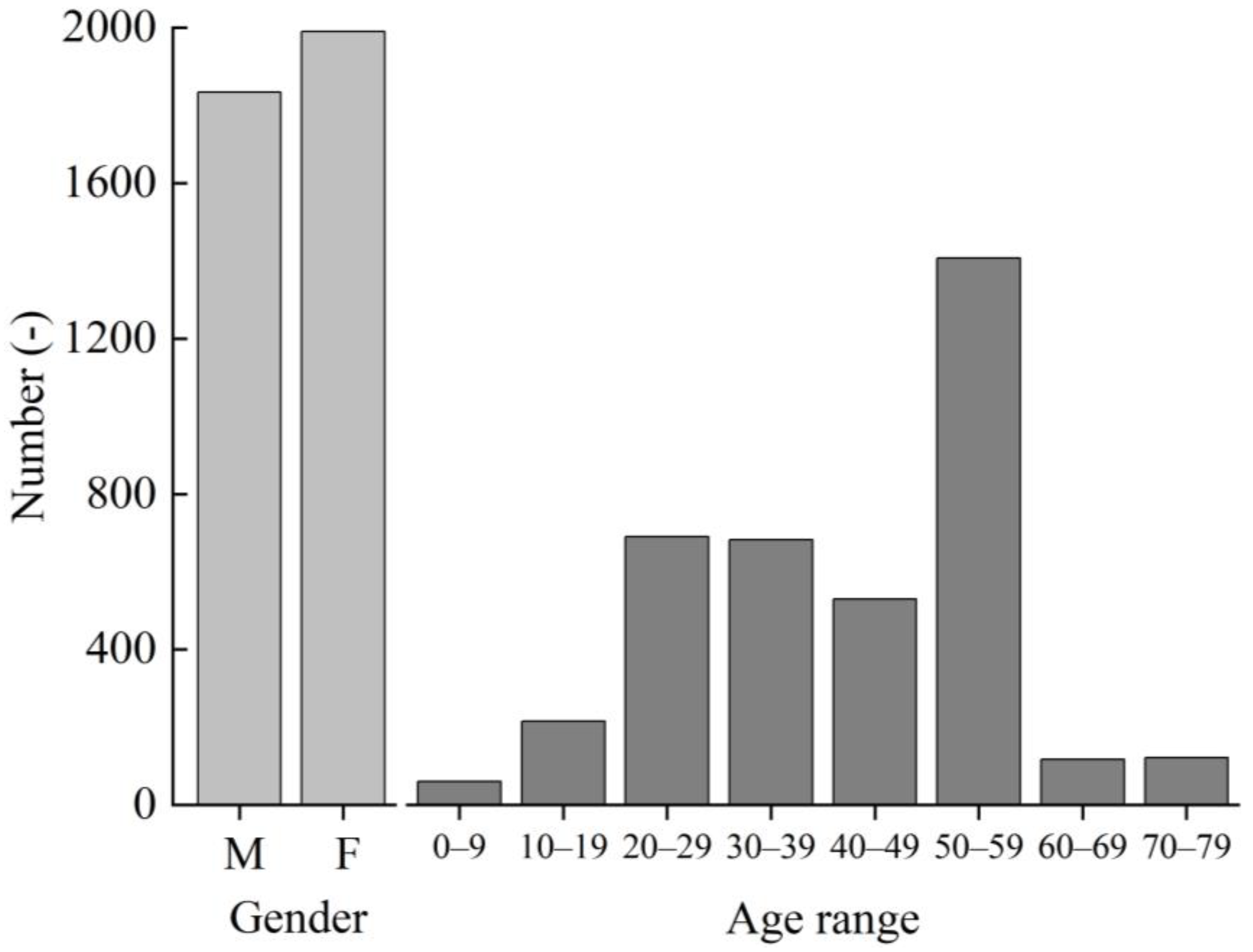
The survey was conducted from 1 December 2010 to 28 February 2011. During this period, 3821 votes were collected without missing all the features. A total of 65 participants took part in the survey, with 30 units being included in the study. Among the participants, there were 32 males and 33 females. The age of the participants ranged from 7 to 79 years, with an average age of 41.1 years.

Table 2. Gender and age distribution of survey participants.

Gender		Age Group
Male	Female	0–9	10–19	20–29	30–39	40–49	50–59	60–69	70–79	80+
32	33	2	3	13	12	8	23	2	2	0

shows the age and gender distribution of the survey participants in the winter analysis.

During the actual measurement period of the indoor thermal environment, questionnaires were administered regarding the participants’ occupant behavior four times a day. Each of the four surveys necessitated a report for distinct time periods: from waking until 12:00, 12:00 to 16:00, 16:00 to 20:00, and 20:00 until bedtime. However, if it was difficult to respond within the allotted time, respondents were allowed to respond at any interval of at least one hour. The survey was administered to individuals who agreed to participate after being informed of the survey’s content in advance. Anonymity was maintained during the study to avoid any personal exposure of participants. The questionnaire used in this study was in Japanese because the participants were Japanese.

3.2. Thermal Environmental Data Collection

The air temperature, relative humidity, and globe temperature were measured in the thermal environment of a room. The survey asked about opening/closing windows, heating, opening/closing interior doors, opening/closing curtains, and kotatsu use. To capture the indoor environment, measurements of the indoor air temperature, relative humidity, and globe temperature were taken at a height of 600 mm, as the living room was designated as the seating area at floor level.

To measure the temperature difference between the height of the floor seat and the feet, the foot temperature was measured at a height of 100 mm, which is the height of the ankles. The measuring instruments were installed in a location that was not affected by solar radiation or heat generation and did not interfere with daily life. In the case of indoor wind speed, measurements were conducted for a duration of 5 min following the initiation of the survey, and the resulting average value was utilized as the representative measure. No anemometers were installed for continuous indoor measurement because the number of anemometers was limited. Due to equipment limitations, the subjects were divided into three groups, with each group being measured approximately 10 days per month. Photographs of the measurement equipment used to measure the indoor air temperature, globe temperature, and indoor relative humidity are shown in Figure 6, and an overview of the measurement equipment is presented in

Table 3. Summary of the measurement equipment.

Parameter	Instrument	Resolution	Accuracy	Manufacturer
Air temperature	Thermo Recorder TR-71	0.1 °C	±0.3 °C	T&D Corporation
Air temperature	Thermo Recorder TR-72	0.1 °C	±0.3 °C
Relative humidity		1%	±5%
Globe temperature	Globe Thermometer 150 mm φ	–	–	SIBATA

.

Two variables associated with the human body were assessed: clothing insulation and the rate of metabolism. The measurement of anthropometric factors was completed by the participants themselves when they answered the subjective report. Metabolic rates were estimated based on work intensity prior to voting. Clothing insulation was estimated using the Hanada weight method [38] by asking respondents to enter the total weight of the clothing they were wearing.

Publicly available data from the Japan Meteorological Agency [39] were used to determine the outdoor thermal environment. The outdoor temperature, outdoor relative humidity, outdoor wind speed, barometric pressure, cloud cover, and precipitation were tabulated. The observation point was Gifu City, Gifu Prefecture, which is located in the center of the studied residence.

3.3. Thermal Indices

A thermal index was used as a characteristic in this study. The thermal indices employed encompassed the operative temperature (Top), average radiant air temperature (MRT), dew point temperature (Td), modified effective temperature (ET*), standard modified effective temperature (SET*), wet-bulb globe temperature (WBGT), neutral temperature (Tn), and the disparity between the action temperature and neutral temperature (Tdiff). The difference between the operative temperature and 18 °C (T_op-18) was used as a characteristic to analyze the limits of adaptation to cold environments.

The operative temperature is an evaluation index of the thermal environment of the human body. As this study was conducted indoors under calm airflow conditions, the temperature was calculated using the average room air temperature and mean radiant air temperature according to ASHRAE Standard 55 [40].

$$T_{op}=A{t}_a+\left(1-A\right)\overline{t_r}$$

(21)

• T_op = operative temperature (°C)
• t_a = average air temperature (°C)
• t_r = mean radiant air temperature (°C)
• A = constant as a function of air velocity (0.5)

The mean radiant air temperature (MRT) was calculated based on Benton’s formula [41], and the formula for calculating the MRT is given below:

$$T_r={\left(\frac{6.32*D^{-0.4}*v^{0.5}}{\sigma *\epsilon }*\left(T_g-T_a\right)+T_g^4\right)}^{0.25}$$

(22)

• D = diameter of globe thermometer (m)
• ε = emissivity of globe thermometer (0.95)
• σ = Stefan–Boltzmann constant (5.67 * 10⁻⁸ [W/m²K⁴])
• Ta = air temperature (K)
• Tg = globe temperature (K)
• Tr = MRT (K)
• v = air velocity (m/s)

The globe thermometer used in this study was a Vernon type (0.15 m diameter).

The dew point temperature was calculated using Tetens’ formula [42]. The dew point temperature was calculated using the following formula:

$$T_d=\frac{237.3 {\log }_{10}\left(\frac{6.1078}{e}\right)}{{\log }_{10}\left(\frac{e}{6.1078}\right)-7.5}$$

(23)

• Td = dew point temperature (°C)
• e = water vapor pressure in the air (hPa)

The new effective temperature is an evaluation index based on a thermal equilibrium equation. It can comprehensively evaluate the air temperature, humidity, airflow, radiation, clothing insulation, and metabolic rate, and takes into account the thermoregulatory function of the body through sweating using a two-node model. The standard new effective temperature was specified as a standard environment with an air velocity of 0.135 (m/s), metabolic rate M (met), and standard clothing insulation to allow the comparison of thermal environments under different conditions. The new effective temperatures were obtained from the ASHRAE thermal comfort tool, and the standard new effective temperatures were obtained from ASHRAE Standard 55 [40]. Atmospheric pressure data for Gifu City, Gifu Prefecture, Japan, were obtained from the Japan Meteorological Agency [39]. Body weight data were obtained from the Ministry of Health, Labor, and Welfare [43], and body surface area was calculated using the Kurazumi formula [44]. The Kurazumi formula is as follows:

$$S=72.18 * W^{0.425} *{ H}^{0.725}$$

(24)

• S = body surface area (cm²)
• W = weight (kg)
• H = height (cm)

The WBGT was proposed in the United States in 1954 to prevent heat stroke in U.S. military personnel. The WBGT is an index that focuses on the heat exchange between the human body and the outside air and takes into account humidity and solar radiation, which have a great influence on the heat balance of the human body. The calculation formula is as follows:

$$\mathrm{W}\mathrm{B}\mathrm{G}\mathrm{T}={0.7T}_w+0.3T_g$$

(25)

• Tw = wet-bulb temperature (°C)
• Tg = globe Temperature (°C)

The neutral temperature is the operative indoor temperature at which occupants are comfortable, as dictated by temperature/cooling sensation. There are two methods for calculating neutral temperature: linear regression and the Griffith method [45]. The Griffith method is generally used because linear regression methods are susceptible to highly biased data. The formula for calculating the neutral temperature using the Griffith method is as follows:

$$T_n=T_i+\frac{0-TSV}{a}$$

(26)

• Tn = neutral temperature (°C)
• Ti = room air temperature (°C)
• TSV = thermal sensation vote (-)
• A = sensitivity constant (0.5)

4. Results and Discussion

4.1. Basic Aggregation

The results of the survey in this study were tabulated. A total of 3821 votes were collected. Figure 7 shows the distribution of the gender and age of residents in the received votes. The survey involved the participation of approximately an equal number of males (1833) and females (1988), resulting in a near 1:1 ratio. The age distribution of the survey participants was primarily characterized by individuals in their 50s, followed by those in their 20s.

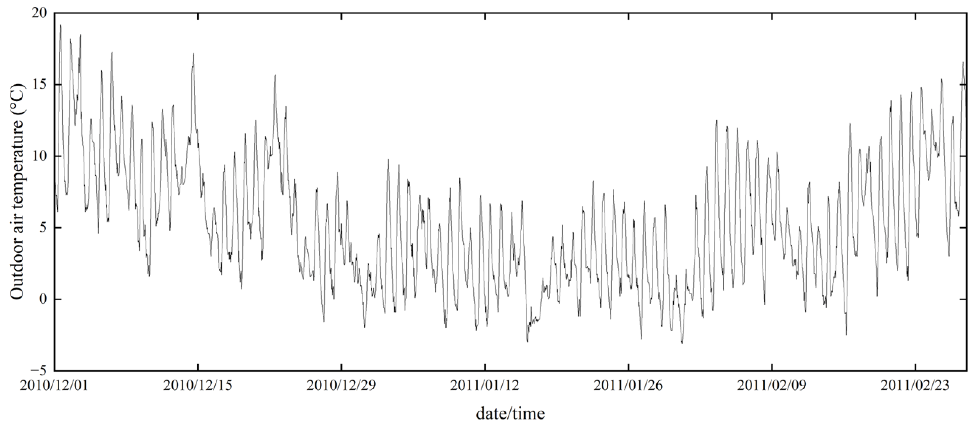
Figure 8 shows the outdoor air temperature trends in Gifu City during the study period.

Table 4. Statistical summary of thermal environment data and thermal comfort indices.

	Feature	Mean	Max.	Min.	Median	S.D.
Indoor	Air temperature (°C)	15.7	28.5	−0.5	16.5	4.65
	Relative humidity (%)	53.5	89	19	53	10.56
	Air velocity (m/s)	0.1	0.1	0.1	0.1	0.00
	Globe temperature (°C)	15.1	32.1	−1.6	15.8	4.55
	Wet-bulb temperature (°C)	10.6	19.9	−1.6	11.1	3.75
	Foot temperature (°C)	13.3	23.2	−0.5	13.8	3.84
Outdoor	Air temperature (°C)	4.7	18.5	−3.1	4	4.10
	Relative humidity (%)	66.0	91	15	68	15.64
	Air velocity (m/s)	2.4	10.9	0	1.9	1.61
	Atmospheric pressure (hPa)	1014.1	1025.2	997.9	1015.4	6.05
	Cloud cover (-)	6.9	10	0	9	3.79
	Precipitation (mm)	0.1	11.5	0	0	0.63
Thermal index	Operative temperature (°C)	15.4	29.1	−0.6	16.2	4.58
	MRT (°C)	15.1	32.1	−1.6	15.8	4.55
	Dew point temperature (°C)	6.0	18.1	−6.7	6.2	4.39
	WBGT (°C)	11.9	21.5	−1.3	12.6	3.93
	ET* (°C)	16.1	32.8	−0.5	16.6	5.00
	SET* (°C)	17.8	36.9	−3.9	17.9	6.69
	Neutral temperature (°C)	17.7	29.1	1.4	18.4	4.37
	Tdiff (°C)	−2.3	2	−8	−2	1.94
	Top-18 (°C)	−2.6	11.1	−18.6	−1.8	4.59
Human factor	Metabolic rate (met)	1.3	2	0.8	1.2	0.39
	Clothing insulation (clo)	0.8	2.7	0.3	0.7	0.32

MRT, mean radiant air temperature; WBGT, wet-bulb globe temperature; ET*, new effective temperature; SET*, standard new effective temperature; Tdiff, difference between operative temperature and neutral temperature; T_op-18, difference between 18 °C and current T_op.

also provides a statistical summary of the indoor and outdoor thermal environments and thermal comfort index. The minimum and maximum indoor air temperatures were −0.5 °C and 28.5 °C, respectively, with an average value of 15.7 °C. The minimum and maximum indoor relative humidity values were 19% and 89%, respectively, with an average value of 53.5%. The indoor thermal environment was similar to that of a typical Japanese house during winter. The minimum outdoor air temperature was −3.1 °C, the maximum was 18.5 °C, and the mean was 4.7 °C. The minimum and maximum outdoor relative humidity values were 15% and 91%, respectively, with an average value of 66.0%. The outdoor thermal conditions mirrored the overall winter climate of Gifu City.

Table 5. Indoor environmental conditions in the poll during the period.

Occupant Behavior	Number	On (Open)	Off (Close)
Heating	3821	2442	1379
Window	3821	112	3709
Door	3821	611	3210
Curtain	3821	1263	2558
Kotatsu	3821	1019	2802

lists the indoor environmental conditions indicated by the votes during this period. Approximately 64% of the respondents were using heating at the time they cast votes during this period. In addition, the results were low for open windows and interior doors in the living room during the winter months. Approximately 33% of the curtains were open at the time of voting. The kotatsu was in use approximately 26.5% of the time at the time of voting. A higher percentage of openings were closed during the winter months to improve the air-tightness of the rooms. The percentage of respondents who used a heater was higher than those who used a kotatsu, indicating that the use of a heater is common in homes.

Table 6. Statistical summary of subjective votes in the winter analysis.

Subjective Vote	Proportion (%)
Thermal sensation	Cool	Neutral	Warm
	32.0	68.0	0.0
Thermal conscious	Unconscious		Conscious
	37.6		62.4
Thermal acceptability	Unacceptable		Acceptable
	12.3		87.7
Thermal tolerance	Intolerable		Tolerable
	9.7		90.3
Affective assessment	Uncomfortable		Comfortable
	18.9		81.1
Thermal preference	Cooler	No change	Warmer
	0.2	34.3	65.5

provides a statistical summary of the subjective votes. In tabulating the data, a reclassification was made in terms of thermal sensation and affective assessment. For thermal sensation, “very cold”, “cold”, and “cold” were classified as cold, with scale values from −4 to −2; “slightly cold”, “neither hot nor cold”, and “slightly warm” were classified as neutral, with scale values from −1 to +1; and “warm”, “hot”, and “very hot” were defined as hot, with scale values from +2 to +4. When rating the affective assessment, “very uncomfortable”, “extremely uncomfortable”, and “unpleasant” were classified as unpleasant, with scale values from +1 to +3, and “somewhat uncomfortable” and “comfortable” were considered comfortable, with scale values from +4 to +5. In the winter indoor environment, there were only votes for “cold” or “neutral” and no votes for “hot”.

4.2. Analysis According to Initial Conditions

Machine learning has been shown to be effective for many predictions due to its high accuracy and ease of use in analyzing training data [46]. For this reason, a number of studies have been conducted using machine learning techniques to predict energy consumption and analyze the impact of energy conservation measures such as renewable energy technologies [47,48,49]. Although machine learning has been used extensively in predicting building energy consumption, few analyses have been conducted on predicting occupant behavior using machine learning. Machine learning varies in its ease of use, ability to build predictive models with interpretable structures, and computational cost, depending on the method [50]. Therefore, it is imperative to explore the utilization of machine learning models in order to ascertain the optimal approach for predicting the behavior of residents when it comes to opening and closing windows.

First, the analysis was performed under the initial conditions using three machine learning models: logistic regression (LR), SVM, and DNN. The initial conditions were analyzed using all features and no parameter tuning. A total of 37 features were used in the analysis. The features used in the analysis are listed in

Table 7. Features used in the winter analysis.

		Features
Thermal environmental data	Indoor	Indoor air temperature, indoor relative humidity, indoor air velocity, globe temperature, wet-bulb temperature, foot temperature
	Outdoor	Outdoor air temperature, outdoor relative humidity, outdoor air velocity, atmospheric pressure, cloud cover, precipitation
Thermal comfort indices		Operative temperature, MRT, dew point temperature, WBGT, ET*, SET*, neutral temperature, Tdiff, Top-18
Subjective vote		Thermal sensation, thermal conscious, thermal acceptability, thermal tolerance, affective assessment, thermal preference
Human factor		Gender, age, metabolic rate, clothing insulation, posture
Occupant behavior		Window, door, curtain, kotatsu
Other		Date/time

.

The default values were used for the parameters of the initial conditions, which are in machine learning. For the LR, no parameter tuning was performed because no parameters could be set. For SVM, gamma and C are tunable parameters. The values used for the initial conditions were gamma = 0 and C = 0. A DNN has parameters that can be tuned by the layers and neurons. The values used for the initial conditions were layer = 2 and neuron = (50, 50).

Table 8. Comparison of accuracies of machine learning models as a function of initial conditions.

	Accuracy	Precision	Recall	F-Measure
LR	0.783	0.862	0.787	0.823
SVM	0.770	0.829	0.807	0.818
DNN	0.827	0.882	0.843	0.862

shows a comparison of the accuracies of the machine learning models as a function of the initial conditions.

Under the initial conditions, the accuracies were 0.783, 0.770, and 0.827 for LR, SVM, and DNN, respectively. When comparing the three machine learning models, DNN showed the best accuracy, but no significant differences were found when compared to LR or SVM. In addition, the fact that extremely low values for precision, recall, and F-measure were not obtained indicates that the machine learning models’ predictions were not biased toward either “heating on” or “heating off”. Thus, the validity of the machine learning models was confirmed in this study. It needs to be investigated to what extent the accuracy can be improved through feature selection and parameter tuning.

4.3. Analysis by Feature Selection

4.3.1. Machine Learning Features

Feature selection was performed to analyze the features that affect the use of winter heating. Feature selection was performed in two ways, forward selection (FS) and backward elimination (BE), which are widely used in machine learning. FS is a method that starts with no features and increases the number of features individually to find the most accurate combination. BE is a method that starts with all the features included and decreases the number of features one by one to find the most accurate combination. The objective was to investigate the difference in accuracy between the two methods and the combination of common features.

Table 9. Comparison of the evaluation indices by feature selection.

Models	Feature Selection	Accuracy	Precision	Recall	F-Measure
LR	FS	0.795	0.872	0.796	0.832
	BE	0.795	0.871	0.798	0.833
SVM	FS	0.793	0.810	0.884	0.845
	BE	0.802	0.813	0.898	0.853
DNN	FS	0.843	0.891	0.860	0.875
	BE	0.847	0.896	0.861	0.878

shows a comparison of the accuracy by feature selection.

There was no difference in the prediction accuracy between FS and BE in the LR, SVM, and DNN models. Compared to the initial accuracy, LR’s accuracy increased by approximately 1.5%, SVM’s increased by approximately 2.9% to 4.2%, and DNN’s increased by approximately 1.9% to 2.4%. Although feature selection improved the accuracy, it did not produce the expected results in predicting resident behavior.

Table 10. Features selected for forward selection and backward elimination.

			LR		SVM		DNN
			FS	BE	FS	BE	FS	BE
Thermal environmental data	Indoor	Air temperature	0	0	0	0	1	1
		Relative humidity	1	0	1	1	1	1
		Air velocity	1	1	0	0	1	1
		Globe temperature	0	1	0	0	0	1
		Wet-bulb temperature	1	0	0	0	1	1
		Foot temperature	1	1	0	0	1	1
	Outdoor	Air temperature	1	1	1	1	1	1
		Relative humidity	1	0	1	0	0	0
		Air velocity	0	0	0	0	1	0
		Atmospheric pressure	1	0	1	0	1	1
		Cloud cover	0	1	0	0	0	0
		Precipitation	0	0	0	0	1	1
Thermal comfort indices		Operative temperature	1	0	0	0	1	0
		MRT	1	0	0	0	1	1
		Dew point temperature	0	1	0	1	0	1
		WBGT	1	0	0	0	1	1
		ET*	1	1	0	0	0	1
		SET*	0	1	0	0	0	1
		Neutral temperature	1	0	0	0	1	0
		Tdiff	0	1	0	0	0	1
		Top-18	0	0	1	0	1	1
Subjective vote		Thermal sensation	1	1	1	1	1	1
		Thermal conscious	0	1	1	0	1	1
		Thermal acceptability	1	1	1	0	1	1
		Thermal tolerance	1	0	1	1	1	1
		Affective assessment	0	0	1	1	1	1
		Thermal preference	1	0	1	0	1	1
Human factor		Gender	0	0	1	0	1	1
		Age	1	1	1	1	1	1
		Metabolic rate	0	0	1	0	1	1
		Clothing insulation	0	0	0	0	0	1
		Posture	1	1	1	1	1	1
Occupant behavior		Window	1	1	1	1	1	1
		Door	1	1	1	1	1	1
		Curtain	0	0	1	1	1	1
		Kotatsu	1	1	1	1	1	1
Other		Date/Time	1	1	1	1	1	1

A 1 indicates that the feature was selected in FS and BE. A 0 indicates that the feature was not selected in FS and BE.

lists the selected features in FS and BE. With the exception of relative humidity, no indoor thermal environment features were selected for the SVM. In the DNN, however, features were selected for the indoor thermal environment, except for the FS globe temperature. Thermal indicators were selected infrequently for the SVM, but irregularly for LR and the DNN. Occupant behavior was selected for all but the LR curtain. The DNN selected a relatively large number of features for both FS and BE, whereas the SVM tended to select fewer features compared to the DNN. There was no regularity in the features selected for the LR, SVM, or DNN models. There was also no difference in the selected features between FS and BE.

4.3.2. Examination of Features through Linear Regression

In the previous section, machine learning was used to select features. However, no regularity was found in the selected features. In this section, linear regression is performed on the features used in machine learning to analyze the relationships between the features and the features that affect heating usage.

Table 11. Comparison of indicators by linear regression.

			Coefficient	Std. Error	t-Stat	p-Value
Thermal environmental data	Indoor	Air temperature	0.362	0.002	235.1	0.000
		Relative humidity	0.012	0.001	20.7	0.000
		Air velocity	−0.001	NaN	NaN	NaN
		Globe temperature	0.083	0.002	54.8	0.000
		Wet-bulb temperature	−0.093	0.002	−48.6	0.000
		Foot temperature	−0.043	0.002	−25.7	0.000
	Outdoor	Air temperature	−0.036	0.002	−23.8	0.000
		Relative humidity	−0.001	0.000	−1.8	0.072
		Air velocity	0.008	0.004	2.1	0.038
		Atmospheric pressure	0.000	0.001	0.0	0.996
		Cloud cover	−0.001	0.002	−0.4	0.703
		Precipitation	0.013	0.010	1.4	0.175
Thermal comfort indices		Operative temperature	−0.143	0.002	−92.7	0.000
		MRT	0.083	0.002	54.4	0.000
		Dew point temperature	0.030	0.002	18.8	0.000
		WBGT	−0.036	0.002	−19.8	0.000
		ET*	−0.013	0.001	−9.1	0.000
		SET*	0.027	0.001	26.1	0.000
		Neutral temperature	−0.101	0.002	−67.2	0.000
		Tdiff	−0.044	0.003	−12.7	0.000
		Top-18	−0.149	0.002	−96.7	0.000
Subjective vote		Thermal sensation	−0.022	0.007	−3.2	0.001
		Thermal conscious	−0.007	0.013	−0.6	0.560
		Thermal acceptability	0.033	0.019	1.7	0.087
		Thermal tolerance	0.118	0.022	5.4	0.000
		Affective assessment	0.008	0.008	1.0	0.305
		Thermal preference	0.022	0.013	1.6	0.100
Human factor		Gender	0.024	0.012	2.0	0.049
		Age	−0.003	0.000	−6.4	0.000
		Metabolic rate	−0.115	0.016	−7.2	0.000
		Clothing insulation	−0.255	0.019	−13.2	0.000
		Posture	−0.014	0.002	−6.4	0.000
Occupant behavior		Window	−0.269	0.037	−7.3	0.000
		Door	−0.204	0.017	−11.9	0.000
		Curtain	0.098	0.013	7.5	0.000
		Kotatsu	0.071	0.014	5.1	0.000
Intercept			−2.892	Infinity	0.0	1.000

shows the values obtained using linear regression.

The coefficient of determination, standard error, t-value, and p-value were used as the indices for linear regression. The coefficient of determination indicates the degree of fit of the estimated regression equation; the closer it is to 1, the stronger the explanatory power for the target variable. The standard error is the standard deviation of the estimator and represents the variability of the estimator obtained from the sample. The t-value and p-value are indicators of the statistical significance or dominance of the coefficient of determination for a feature. For a feature to reach the 5% significance level, the absolute value of the t-value must be greater than 2 or the p-value must be less than 0.05.

No linear regression index could be determined for the characteristic room air velocity because only representative values from 5 min of measurements were used due to the availability of equipment. For acceptance and preference, precipitation, comfort, barometric pressure, cloud cover, indoor awareness, and outdoor relative humidity, the absolute t-values were greater than 2 and the p-values were greater than 0.05. Therefore, these features did not appear to have a statistically significant effect on heating use.

The highest coefficient of determination was 0.362 for indoor air temperature. In addition, features such as thermal tolerance, curtains, and globe temperature were observed to have a positive influence on heating use. Clothing insulation and interior doors also had negative coefficients of determination, which may have resulted in a negative influence on heating consumption. The highest absolute value of the coefficient of determination was obtained for indoor air temperature, suggesting that indoor air temperature is the feature that has the greatest influence on heating use among the features used in this study.

Linear regression showed the features that influenced heating use. In addition, feature selection using machine learning revealed the feature combinations that yielded the highest accuracy. While the summer analysis showed that the trade-off features had a significant influence on the objective variable, the winter analysis did not identify any features with a particularly large effect.

4.4. Analysis by Parameter Tuning of SVM

Because no significant improvement in prediction accuracy was observed with feature selection, parameter tuning was performed. The purpose of parameter tuning is to maximize the estimation performance of unknown data by balancing the nonlinearity and generalization ability of the machine learning model with the parameters. There are two parameters in SVM: C and gamma. Because the range of parameters can be set infinitely, it is difficult to find the point where the prediction accuracy is maximized. For this analysis, the parameters were set on a logarithmic scale, and a grid search was performed to find the maximum prediction accuracy over a wide range. Eleven Cs were set (10^N, N = −1 to 9), with a global minimum of 10⁻¹ and a global maximum of 10⁹, and 11 gamma rays were set (10^N, N = −6 to 4), with a global minimum of 10⁻⁶ and a global maximum of 10⁴. In the analysis of the initial conditions, the precision, recall, and F-measure values did not show any problems with data imbalance. Therefore, in the parameter tuning analysis, accuracy was used to study the forecast accuracy. 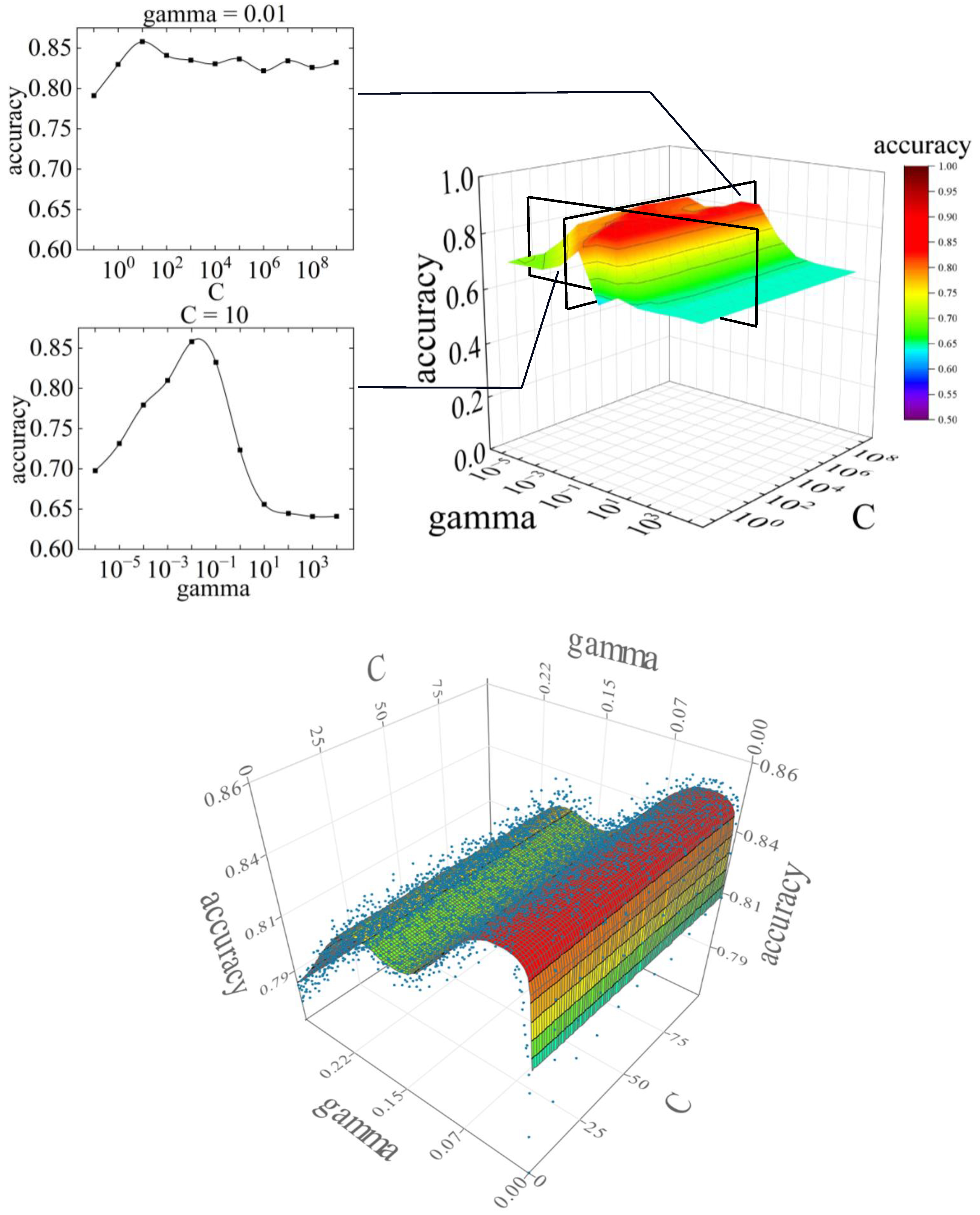Figure 9 shows the variation in accuracy in the difference between C and gamma, and the variation in accuracy represented by the response surface. The relationship between C and accuracy at a fixed gamma is shown in Figure 10, and the relationship between gamma and accuracy at a fixed C is shown in Figure 11.

The parameter tuning results showed that accuracy was highest at C = 10¹ and gamma = 10⁻². The accuracy at gamma = 10⁻² was above 0.82, except at C = 10⁻¹, suggesting that larger values of C do not significantly affect the prediction accuracy. However, the accuracy of gamma varied compared to C, which may have significantly affected the prediction accuracy.

The response surfaces were created and optimized based on the accuracy obtained by tuning the SVM parameters. The response surface is a model that approximates the relationship between the predictor variables and the predicted response. The computational optimization time can be significantly reduced by using the response surface method. Evolutionary design, an approximation method, was used for the response surface technique. Evolutionary design is a method that uses genetic algorithms to search for optimal combinations of elementary functions. The predictor variables were C and gamma, which are SVM parameters, and accuracy was used for the response. Ten values of C were set on a linear scale, with a global minimum of 1 and a global maximum of 100. Three hundred gamma values were set on a linear scale, with a global minimum of 0.001 and a global maximum of 0.3. The optimality obtained for the response surface ranged from gamma = 0.0289 to 0.0346, with an accuracy of 0.8486. The value of C did not affect the accuracy.

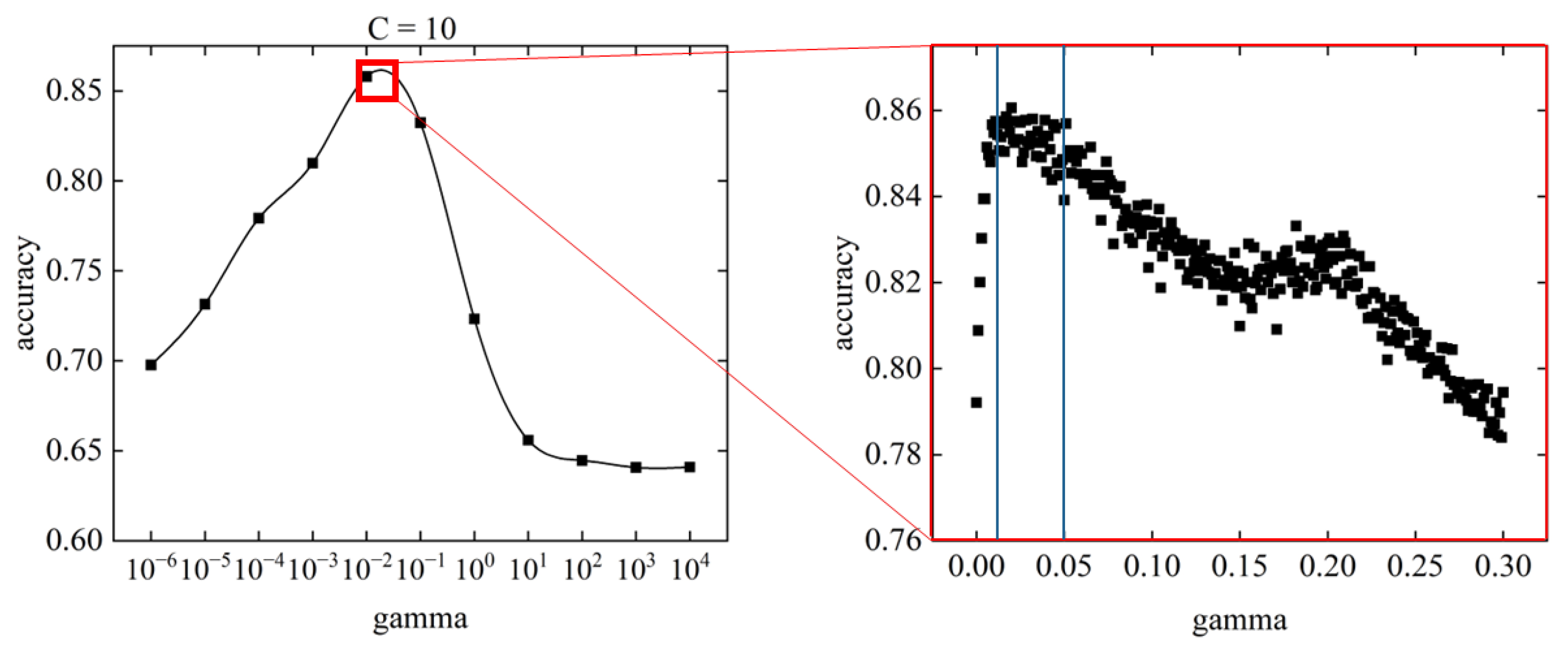
When tuning the parameters of the SVM, the value of gamma was found to have a greater influence on the prediction accuracy compared to the value of C. Therefore, we set the value of C to 10, where the best value was obtained, and tuned the gamma value by decreasing the range. Because the local maximum of the gamma was found near 10⁻², 300 gamma values were set on a linear scale, with a global minimum of 0.001 and a global maximum of 0.30. Figure 12 shows the relationship between gamma and accuracy at C = 10.

The range of gamma where the accuracy was highest was between gamma = 0.01 and gamma = 0.05, the range indicated by the blue line in the figure. The point with the highest accuracy was in the range from gamma = 0.01 to gamma = 0.05, specifically gamma = 0.028, with an accuracy of 0.862. All points within this range had accuracies greater than 0.84, indicating high prediction accuracy. In the gamma range above 0.05, the accuracy tended to decrease with increasing gamma. A local maximum in the accuracy occurred around gamma = 0.2, but it was not a global maximum.

The prediction accuracy obtained through SVM parameter tuning had a global maximum value of 0.862. The prediction accuracy of the SVM initial conditions was 0.770, which means that parameter tuning improved the prediction accuracy by approximately 11.9%. Parameter tuning may be effective in improving the fit to unknown data in occupant heating behavior.

4.5. Analysis through Parameter Tuning of the DNN

Similar to the parameter tuning for the SVM, parameter tuning was also performed for the DNN to investigate the prediction accuracy. There are two DNN parameters: the layer and the neuron. The larger the values of the layers and neurons, the more complex the interior of the hidden layer becomes. Therefore, it is necessary to consider the values of the layers and neurons that yield the highest prediction accuracy. In addition, because the DNN is a black-box model, the computational process of the hidden layer is not revealed. Instead, it is expected to have higher prediction accuracy compared to the white-box models. Figure 13 shows the change in accuracy for different numbers of layers and neurons. Figure 14 shows the relationship between the number of layers and accuracy when the number of neurons is fixed, and Figure 15 shows the relationship between the number of neurons and accuracy when the number of layers is fixed.

When the number of neurons = 1, the accuracy decreased as the number of layers increased. When the number of neurons = 100 to 600, there was no significant change in accuracy as the number of layers changed. When the number of neurons = 700 to 1000, the accuracy was stable until the number of layers was about six but became unstable as the number of layers increased beyond seven.

The DNN showed excellent prediction accuracy when the number of layers = 2–6 and the number of neurons = 200–500, indicating that too small or too large values for the layer and neuron parameters can have a negative effect on the prediction accuracy. The highest accuracy achieved by parameter tuning was 0.847, and the accuracy under the initial conditions of the DNN, i.e., with the number of layers = 5 and the number of neurons = 200, was 0.827, which improved the prediction accuracy by approximately 2.4%. Because the accuracy under the initial conditions of the DNN was higher than that of the other machine learning models, the expected prediction accuracy was not achieved in parameter tuning.

Compared to SVM parameter tuning, DNN parameter tuning resulted in a lower rate of increase in accuracy. DNNs provide relatively high prediction accuracy without parameter tuning, which should allow for easy verification of accuracy in future analyses. In contrast, the SVM outperformed the DNN in terms of accuracy after parameter tuning, confirming the importance of parameter tuning in SVM. In future studies of prediction accuracy in resident behavior, the tuning of SVM parameters may help improve prediction accuracy.

The accuracy obtained by tuning the DNN parameters was used to create and optimize the response surface. Evolutionary design, an approximation method similar to SVM, was used for the response surface method. The DNN parameters (neuron and layer) were used as the predictor variables, and accuracy was used as the response. Ten neuron values were set on a linear scale, with a global minimum of 1 and a global maximum of 1000. Ten layer values were set on a linear scale, with a global minimum of 1 and a global maximum of 10.

The response surface of the DNN, obtained using the evolutionary design, is shown in Figure 13. The DNN showed more stable values for prediction accuracy over a wider range compared to the SVM. The neurons achieved high prediction accuracy mainly in the range of 200 to 600, whereas the layers achieved high prediction accuracy in layers 5 and 6. For both the neurons and layers, the response surface showed that the prediction accuracy decreased above a certain value.

4.6. Time-Series Changes in Forecast Accuracy Due to Parameter Tuning

To investigate the relationship between the time series and forecast accuracy during the study period, the daily and weekly forecast accuracies were determined. The machine learning model used was SVM, and the parameters were C = 10 and gamma = 0.028, which showed the best accuracy. Figure 16 shows the change in the forecast accuracy over time on a daily basis, and Figure 17 shows the amount of data on a daily basis. Figure 18 shows the change in the forecast accuracy over time from week to week, and Figure 19 shows the amount of data from week to week. Although there were daily variations in the accuracy values, there was no significant variation in the forecast accuracy of the time series, with values averaging close to 0.8. The first week of December and the first and second weeks of January also showed high forecast accuracy, with values above 0.90. While the accuracy of the forecast for the first week of January may have been affected by the small amount of data, the accuracy for the first week of December was high, despite the large amount of data. This suggests that seasonal changes in early December may improve the accuracy of the heating consumption forecasts.

5. Conclusions

This study investigated the prediction accuracy of occupant behavior using machine learning with thermal environment training data measured in a house in Gifu City.

The heating behavior of the occupants in the winter months was predicted. We analyzed the factors affecting heating behavior and performed parameter tuning in machine learning models to examine their accuracy. For feature selection, FS and BE were performed using machine learning. Compared to the baseline, the prediction accuracy improved, but only by 1.5% to 4.2% for LR, SVM, and DNN. Linear regression analysis was also performed to analyze the effects of the features on heating use. Indoor air temperature was the feature that most strongly influenced heating use, with a coefficient of determination of 0.362, but no features were found to have a particularly large effect on heating use.

Parameter tuning of the SVM showed that the values of C and gamma affected the prediction accuracy. The value of gamma was found to have a greater influence on the features than the value of C. Accuracy was highest at 0.862 when C = 10 and gamma = 0.028. Compared to the baseline condition, the prediction accuracy improved by approximately 11.9%, confirming the effectiveness of using parameter tuning in SVM.

Parameter tuning of the DNN showed that the values of the layers and neurons affected the prediction accuracy. Excellent prediction accuracy was observed for layers 2–6 and neurons 200–500. The highest accuracy value was 0.847 when the number of layers = 5 and the number of neurons = 200. Although parameter tuning also improved the prediction accuracy of the DNN, the rate of increase was lower than that of the SVM.

The time-series change in the forecast accuracy after parameter tuning showed high accuracy in the first week of December, the first week of January, and the second week of January. In early January, the small amount of data could have affected the accuracy of the forecast, whereas in early December, the forecast accuracy was high despite the relatively large amount of data. This is expected to improve the accuracy of predicting occupant heating consumption in early December as the season changes.

Future issues that need to be addressed include the following.

Improved accuracy of forecasting models:

Machine learning models that have been widely used in previous studies were used, but there are other models besides those used in this study. In addition, parameter tuning was performed on only two models: SVM and DNN. Therefore, considering the machine learning model and parameter tuning methods used may contribute to further improvements in forecast accuracy. Feature selection also affects prediction accuracy. It is possible that the features not measured in this study have a significant impact on occupant behavior. Although a large amount of data should be collected through new surveys to improve forecasting accuracy, it is also necessary to study the features before the survey.

Automatic schedule generation based on lifestyle considering time history:

Because this study was based on point data at the time of the poll, time history was not taken into account, and we could not get to the point where the daily schedule could be clarified. Accurate surveys of the living environment and analyses using line data from continuous measurements are needed.