A Machine Learning Pipeline to Forecast the Electricity and Heat Consumption in a City District

Abstract

The shift towards renewable energy integration into smart grids has led to complex management processes, which require finer-grained energy and heat generation/ demand forecasting while considering data from monitoring devices and the integration of smaller multi-energy sub-systems at the community, district, or buildings level. However, energy prediction is challenging due to the high variability in the electrical and thermal energy demands of building occupants, the heterogenous characteristics of the energy assets or buildings in a district, and the length of the forecasting horizon. In this paper, we define a data-driven machine-learning pipeline to predict the electricity and thermal consumption of buildings and energy assets from a city district in 24 h intervals. Each pipeline’s step is divided into sensors’ data processing and model integration, data enrichment and features engineering, and multilayer perceptron model training. To address some of the drawbacks of using the multi-layer perceptron model, such as slow convergence rate and risk of overfitting, and to ensure a lower error in the energy prediction process features, an engineering technique was employed. We incorporated weather data features and interaction features derived from fusing the energy data with statistical models to capture the nonlinear patterns of the electrical and heat demands. The proposed approach was successfully validated in a real-world environment, a city district in Gent, Belgium. It featured good prediction results for electricity and heat production and consumption of various assets without considering the physical characteristics, making it viable and easily applicable in broader urban areas. The evaluation of energy prediction accuracy yielded good results, with a Mean Absolute Error (MAE) falling within the range of 0.003 to 3.27, and a Mean Absolute Scaled Error (MASE) ranging from 7 × 10⁻⁵ to 2.57 × 10⁻³.

1. Introduction

The energy demand is growing at an unprecedented rate due to population growth, urbanization, and industrialization. The shortage of traditional fuel-based energy resources and the ambitious targets for greenhouse gas emissions reductions in Europe is driving a significant shift towards renewable energy. In this context, there is a growing need to decentralize the energy system’s management considering community or district-level sub-systems and to coordinate the energy supply, storage, energy carrier conversion, and consumption within the local geographical area [1]. Such solutions require finer-grained energy generation and demand forecasting that uses Internet of Things (IoT) energy monitoring devices to define programs for integrating buildings and other non-grid-operated energy assets for taking advantage of their flexibility. As the buildings account for a significant amount of district energy consumption and operate at the crossroads of different utility networks, research efforts should focus on transforming them into active players in local grid management [2]. To be effective, such solutions should go beyond the energy efficiency in individual buildings and should consider the potential district-level optimization and interrelations across different energy carriers (e.g., electrical and heat), bearing good estimations of the electrical and thermal energy production and demand [3].

However, finer-grained energy prediction of buildings using regression models is still a challenge due to the high variability in the electrical and thermal energy demands generated by complex factors requiring the consideration of multiple heterogeneous data sources, process temporal, spatial, and computational scalability, and the need for generalization and replicability [4].

Energy forecasting should integrate heterogeneous streams of buildings’ data, making it challenging to combine them effectively in the analysis process [5]. The data-driven black box models offer several advantages, such as machine learning (ML) flexibility and adaptability in using data with heterogeneous structures or content. They may need to consider energy data, weather data, occupancy data, building characteristics, and different types of temporal targets such as hourly or daily energy prediction. This allows for consideration of the complexity of energy systems and the uncertainty of external factors [4]. The district-level energy ecosystem can be complex, with multiple factors affecting electrical and thermal energy consumption and production. Additionally, factors such as economic conditions and social dynamics can impact energy demand, further adding to the complexity. Thus, a substantial amount of historical data, as well as external data sources, are necessary to effectively train ML models for this purpose.

At the same time, there is a need to increase the scalability of energy prediction with the amount, granularity, and velocity of sampled building data, which is an open research direction that requires further investigation [6]. The ML models implemented on data-driven pipelines are more scalable than traditional regression models [7]. They can be trained on big data sets and can handle large volumes of energy data, a feature with which most regression models are struggling because they can become computationally expensive as the size of the dataset increases [8]. Moreover, the ML pipelines can be easily distributed across multiple physical or virtual machines, thus increasing their scalability. Moreover, they have good temporal and spatial scalability and are successfully used for learning and generalizing patterns at different time granularities (hours, days months, etc.) as well as spatial dimensions (i.e., buildings of different dimensions, district level, etc.) [9]. The prediction horizon can also influence forecasting accuracy, the large forecasting horizons being vulnerable to significant uncertainty [10]. Good accuracy results are reported in the literature for one value ahead energy predictions, but as the time horizon grows, the prediction accuracy decreases; thus, efforts should be committed to multi-steps ahead energy prediction aiming to improve the reliability of energy forecasts over longer time horizons.

ML models have good generalization features, being capable of learning complex nonlinear relationships between input variables and output targets. Moreover, they have better replicability when considering a variety of assets or building types from a district. Because they do not require detailed information about the energy assets behind the energy meter, data-driven models can be applied more quickly to a larger number of buildings and assets, making them more easily applicable than physics-informed models. They can successfully support district managers, building owners, and energy stakeholders to decide on energy supply and demand planning, investment, and policy formulation [11]. Moreover, risk mitigation strategies can be defined by relying on data-driven energy forecasting on large geographic scales to help cut carbon emissions, promote renewables as key energy sources, and significantly increase energy system efficiency.

In this paper, we address some of the challenges related to energy prediction by defining a data-driven pipeline based on ML to forecast the electricity and thermal demand of buildings and energy assets from a district in Belgium. We address aspects related to sensors’ data processing and data model integration, data enrichment and features engineering, multilayer perceptron (MLP) model training, and utilization to forecast energy 24 h ahead. The quality and resilience of the model are improved by adding heterogeneous data sources and interaction features into the pipeline, which are engineered by fusing the energy data with statistical models to capture nonlinear electrical and heat demand.

The rest of the paper is organized as follows: Section 2 presents the state-of-the-art approaches to ML models for energy prediction, Section 3 describes the forecasting pipeline, discussing aspects related to data enrichment and feature engineering, Section 4 shows prediction results for electrical and thermal profiles of buildings in a pilot setting while Section 5 concludes the paper and presents future work.

2. Related Work

The energy prediction solutions using data-driven ML aim to learn the forecasting model out of monitored data, making it more adaptable to the uncertain and fast-changing real-world environment [12]. In this context, deep neural networks are extensively used for predicting the energy profiles of various energy assets in the smart grid, due to their good accuracy results.

Salkuti et al. employ artificial neural networks (ANN) for short-term load predictions pairing with differential evolution and wavelet transformations [13]. The ANN captures the nonlinear behavior of the energy consumption data source, wavelet transforms are used to stabilize the time series, and the evolutionary-based differential evolution algorithm is used to solve local minima problems. Viegas et al. couple ANN with genetic algorithms to discover the optimal collection of features for model training and increase the prediction accuracy [14]. Recurrent neural networks (RNN) are designed to process sequential input such as time series of energy data and use their internal state to store and disseminate information between time steps, which is useful when dealing with energy forecasting challenges. A deep RNN technique is employed in [15]. To tackle the uncertainty and volatility of load profiles and to prevent the overfitting problem, customers’ load profiles are clustered into a pool of inputs. They boost the forecasting accuracy on several standard approaches, reducing the mean absolute error.

Even though RNNs can show improvements in forecasting when combined with other techniques, the persistence of the vanishing gradient problem is still a concern. To address this issue, long short-term memory (LSTM) networks are used for load forecasting problems [16] on different prediction horizons and feature selection methods. In [17], LSTM models are compared against backpropagation neural networks showing that they outperform backpropagation models for prediction tasks on both singular consumer load datasets and aggregate grid or substation load. A hybrid approach based on LSTM and convolutional neural networks (CNN) is presented in [18]. LSTM models the sequence in the learning phase and is used to extract features more effectively from the input data. Stratigakos et al. combine LTSM with a Singular Spectrum Analysis (SSA)-based decomposition [19]. Trend, oscillating, and noise components are computed using SSA and employed in a LSTM model enriched with exogenous variables that describe weather conditions. Results show the advantage of LSTM in translating trends and long-term dependencies into accurate energy predictions. Eskandari et al. propose an architecture based on CNN and RNN [20]. CNNs are used for extracting load and temperature features from data, while two-dimensional convolutional kernels are employed for the univariate input to transform it into multidimensional features, which may improve the predicting capacity of RNNs. LSTM networks are used in combination with Prophet [21], indicating a consistent accuracy improvement of energy prediction. Solutions based hybrid or ensemble of neural networks have proven useful for improving the forecasting process in different contexts such as solar power generation prediction [22] or data centers energy demand management [23].

Massaoudi et al. coupled gradient boosting’s benefits with an MLP, lowering the prediction error for renewable energy [24]. The feature engineering technique can improve prediction accuracy by revealing hidden patterns in the data and merging the old findings with the new ones. Multiple different methods for updating the dataset or enhancing it with weather or contextual characteristics, along with an MLP-based strategy, are supported by other papers as effective ways to achieve good results [25,26,27]. Faraji et al. consider the energy and weather data uncertainty and employ a hybrid ML-based forecasting approach that integrates the adaptive neuro-fuzzy inference system, MLP, and radial basis function [25]. The heating and cooling demand of a residential building is predicted using the MLP and support vector regression (SVR) [26]. To improve the prediction accuracy, the authors map the input and output variables linearly and consider building characteristics during training. For predicting heating energy demand, the MLP has better accuracy. SVR, MLP, and CatBoost models are used to define an ML-based hybrid model for energy consumption prediction [27]. The study underlines the need for accurate power load forecasting for energy conservation, lowering power generating costs, and enhancing social and economic benefits. To forecast heating, cooling, and building integrated photovoltaic generation, a multi-objective prediction framework based on ML is proposed in [28]. ANN, support vector machines, and LSTM neural networks are used with good results for a reference office building.

The significant volatility and reliance on randomly initialized parameters characterize ANN prediction performance. To decrease variation in prediction performance corrective approaches based on the autocorrelation of forecasting error and online learning were proposed in [29]. They show better results than existing grey-box and black-box forecasting techniques in a case study of a large building with district energy system characteristics. To provide short-term hourly predictions of building power usage in [30], an ANN model is defined with parameters optimized using Particle Swarm Optimization. Principal Component Analysis selects the relevant modeling inputs and streamlines the model structure. Building energy usage is predicted in [31] using deep neural networks. The rough set theory is employed to decrease the number of input variables and pinpoint relevant aspects influencing energy consumption. The combined rough set and deep neural network technique provide more accurate results than backpropagation and fuzzy neural networks. Wang et al. use a deep CNN for hour-ahead building load forecasting based on ResNet [32]. The model includes a feature fusion technique to improve the model’s capacity for learning as well as an external factor integration branch that accepts weather features as input. The findings show that, in terms of forecasting precision, computational effectiveness and generalization for various buildings, the suggested model performs better than the other models, such as LSTM.

Other hybrid models are evaluated for energy consumption forecasting in smart buildings [33]. The model uses bidirectional LSTMs, RNN stacking, and dropout regularization to anticipate energy usage. Similarly, in [34] the identification of hybrid discriminative features is done using CNNs combined with stacked and bi-directional LSTM networks. CNN is used to extract spatial features, while the stacked LSTM and bi-directional LSTM are used to capture the temporal dependencies in the data. In [35], a prediction model is proposed for sub-item energy consumption in high-rise buildings using the Levenberg–Marquardt algorithm to improve training speed and enable real-time prediction considering hourly average outdoor temperature, humidity, weather characteristics, holidays, wind speed, 24 h a day. Authors of [36] propose a framework for forecasting building energy consumption using deep RNNs. The authors compare four different methodologies for imputing missing data and test the sensitivity of gap size and available data percentage on imputation accuracy. Moreover, they explore the use of deeper networks and regularization methods to overcome the problem of overfitting in deep models. Finally, in [37], the authors propose an adaptive hybrid model based on a genetic algorithm and LSTM neural networks. The adaptive LSTM neural network has better accuracy and resilience than the conventional feedforward neural network considering several variables, including weather profiles and different time horizons.

As presented above, in the state-of-the-art literature, a significant number of prediction models applied to smart grid used cases are reported. Their effectiveness depends on various factors, including the quality and availability of data, the specific characteristics of the energy assets, and the selection and tuning of hyperparameters. However, finer-grained energy prediction of buildings and energy assets is still challenging, especially in real-world environments requiring the consideration of multiple heterogeneous data sources, process temporal, spatial, and computational scalability, and the need for generalization and replicability. The data-driven ML models, as proposed in this paper, have several benefits, such as versatility and suitability for data with diverse structures or content as well as scalability in data processing, and they also have good generation features. The defined pipeline is effective in making energy predictions for various assets (buildings, heat pumps, water treatment, etc.) in a city district as well as for different types and scales of energy (renewable, electrical and heat consumption, etc.). The multilayer perceptron (MLP) model is versatile and can be trained with data at different granularities (15 min, 1 h, etc.) and can provide good prediction results for 24 steps ahead, which is suitable for day ahead planning of the district grid operation [38]. Finally, the pipeline is scalable and able to consider big energy data streams and is more robust and reliable by incorporating diverse data sources and interaction features that are engineered by combining the energy data with statistical models to capture nonlinearities of electrical and heat demand.

3. Materials and Methods

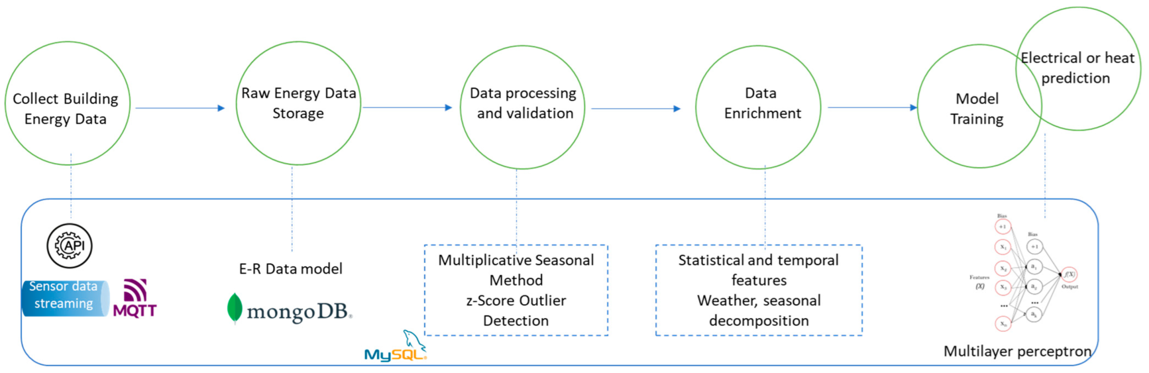
To forecast the electrical and thermal energy profiles of heterogeneous energy assets, we designed an ML-based pipeline, presented in Figure 1.

Figure 1. ML pipeline designed for building energy prediction.

The asset-related data can be acquired by Application Programming Interface (API) calls linked to IoT energy-measuring devices or by directly accessing data storage with energy data. The data may include historical values on load demand or renewable generation and real-time data streams on load consumption patterns for buildings, heat pumps, or other types of assets from a city district. The IoT data sources integration is based on a publish-subscribe broker such as Message Queuing Telemetry Transport (MQTT). The sensors push data through MQTT queues, each to a different topic, and the connection to the MQTT broker is secured using credentials. The format of the received data is a JavaScript Object Notation (JSON) object, and it is stored in a MongoDB database. In this way, records in heterogeneous formats can be safely kept without worrying about the data structure that may change in the future.

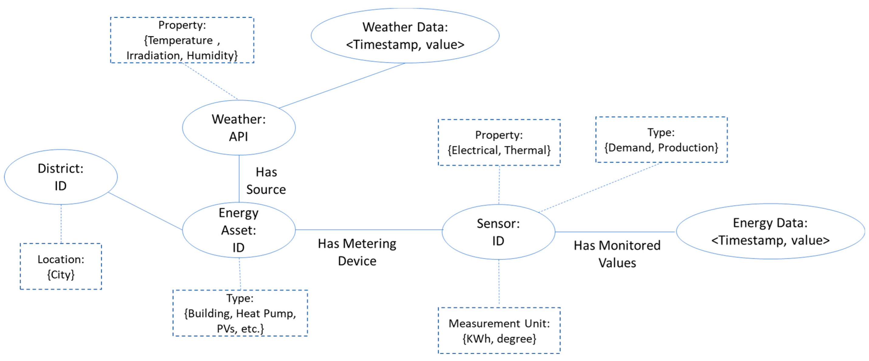
The energy and non-energy data received on the subscribed topics is pre-processed to follow the defined data model structure and then inserted into the appropriate sensor collection (see Figure 2). We use an entity relation data model to store data as immutable time series, also linking it to different relevant properties of the physical asset. In this way, the ML model can benefit from a more comprehensive understanding of the asset’s performance and history over time. A process of cleaning and preparation is carried out to ensure the data’s correctness and consistency.

Figure 2. Data model considered in the prediction pipeline.

The blank or incoherent data points were replaced with values calculated using a missing data imputation method:

$$MSM\left(E_t,d\right)=\frac{\sum _x{\left(\frac{E_t}{\sum _{t=1}^{24}{E}_t}\right)}_{d-x}}{x}$$

(1)

where $d$ represents the duration interval and $x$ represents the number of backwards steps. The missing energy data value $E_t$ is calculated by multiplying the average seasonal factor with the daily average considering several days in the past. The seasonal factor for $E_t$ is calculated by dividing the energy measurement at that hour by the average energy value for that day. In this way, a more complete and reliable dataset is obtained.

The outliers are identified using the z-score method that indicates the deviations in energy data $E_t$ from the mean. It is determined by dividing the difference between the data point and the mean by the standard deviation:

$$z-score\left(E_t\right)=\frac{E_t-\mu }{\gamma }$$

(2)

where μ is the mean and γ is the standard deviation.

As it may have some limitations, such as the sensitivity to extreme values, other methods can be used for normally distributed data (e.g., interquartile range).

The next activity in the pipeline is data enrichment and features engineering (see Figure 1). The accuracy, consistency, comprehensiveness, and applicability of the data used to train the ML model play a significant role in the model’s effectiveness. The quality and resilience of the model may be improved by adding new data sources or features if the data is frequently missing or inadequate. Moreover, to enhance the performance of the model, feature engineering entails choosing and modifying the most important variables or features from the data acquired.

We aim to find and incorporate new data sources relevant to the electricity and heat prediction process. As the pipeline already integrates data on power generation and consumption of district-level buildings and other assets, the integration of weather data is a crucial step to improve the model’s accuracy and create relationships with the energy data. Historical weather data are obtained for the regions of interest, including temperature, humidity, wind speed, solar irradiance, cloud cover percentage, and data describing precipitation amounts. The data were integrated into the pipeline and data model, using the DateTime as the merging variable, while weather data were obtained via API calls (e.g., Visual Crossing Weather API [39]).

The time-related characteristics are also considered since energy consumption and production patterns differ according to the hour of the day, the day of the week, and period of the year. These include the time of day, the day of the week, and the season and lagging features that recorded the energy usage or production over the past several days or hours. This enhanced the accuracy of the model by allowing it to consider the temporal relationships in the data. Outside variables, including vacations and events that may affect load patterns, were considered, in addition to meteorological data. A binary variable indicating whether a particular day was a holiday was included in the dataset as a feature.

Statistical techniques such as the moving average or rolling median have been applied to energy consumption or heat generation to identify trends in energy consumption over time, smooth out any short-term fluctuations in the data, and identify anomalies that may affect the overall trend. The moving average captures the short-term relationships between characteristics and smoothing the energy profiles and was utilized to reduce the impacts of outliers and noise in data. We determined the moving average feature for the previous 6 h and 24 h of energy data observations using the following Simple Moving Average (SMA) formula:

$$SMA\left(E_t\right)=\frac{{\sum }_{t=t-1}^{t=t-n}{E}_t}{n},n=\{6,24\}$$

(3)

The variability in the data was considered using the rolling standard deviation ($\sigma )$ within 24 h. By using it as a feature, the anomalies and hidden load patterns are discovered:

$$\sigma =\sqrt{\frac{1}{24}}\sum _{t=1}^{24}{(E_t-SMA(E_t\left)\right)}^2$$

(4)

The recent trends and patterns in the energy profiles are tracked using a rolling median with a window of 24 h. As new data becomes available, the rolling window moves forward, tracking recent trends and patterns in the energy data. Seasonal effects may have a big impact on the energy patterns. Thus, seasonal adjustment was used to identify and remove the seasonal component of the data, leaving behind the underlying trend and any irregular or unexpected changes in the energy data.

Energy data profiles can be complex to interpret when there is a lot of noise or variability in the data (e.g., residential buildings). A quantitative or statistical measure, the exponentially weighted moving average (EWMA), is utilized to better interpret such energy data profiles. The moving average is designed so that older observations are given lower weights. The parameter $\alpha$ controls the weighting of the current observation in the EWMA computation:

$$EWM{A}_{energy}\left(t\right)=\alpha \times E_t+\left(1-\alpha \right)\times EWM{A}_{energy}(t-1)$$

(5)

We have used the seasonal decomposition approach [40] to split and separate the energy profiles into trend, seasonal, and residual components. Due to their ability to capture many facets of the underlying patterns in the data, each of these elements is used as features in an ML model for energy forecasting. The trend component indicates the long-term changes in the data regardless of seasonality or short-term variations, therefore, using it as a feature allows us to capture a growing or declining trend or a trend that changes direction at predetermined intervals. The hourly trend feature determines the average amount of energy used throughout the day and uses that number to determine the trend component for each hour. This feature can assist the model to capture the daily trends in energy usage or production. The daily trend feature denotes how much energy is typically consumed on each day of the week and uses that number as the trend component for each day. The model can better capture weekly trends in energy use with the aid of this feature, which is crucial for predicting energy demand and production throughout the week. The seasonal component marks the repeated patterns in the data such as daily, weekly, or monthly cycles. Seasonal tendencies in energy use are identified by utilizing the seasonal component as a feature, such as higher energy use during hot summers or cold winters or higher energy use during periods of the day or week. Finally, the residual component holds the randomness in the data that cannot be explained by the trend or seasonal components. By employing the residual component as a feature, we capture unexpected variations in the energy data profiles generated by elements like weather events, sudden shifts in resident behavior, or equipment breakdowns.

To identify more complex patterns and correlations that may not be evident by looking at the energy data alone, interaction features are constructed by combining energy data with moving average, moving median, and rolling standard deviation features (see Table 1). An interaction feature that combines the last energy value with the moving average of the energy observations for a specific time window (24 h in this case) reflects how much current energy usage deviates from the window’s average value, which helps spot abnormalities or shifts in load patterns. We combine energy data and rolling median values to capture the energy patterns that the moving average may miss while the degree of volatility and variability of a specific observation is determined using an interaction feature between energy values and the rolling standard deviation of the previous 24 h. Hourly and daily trends in energy data can provide valuable insights into how energy is produced or consumed over time. The gradient of the energy profiles representing the rate of change in the energy data over a period is used to capture them. Using the gradient as an interaction feature allows the identification of more complex patterns and correlations (see Table 1).

Table 1. Type of features used in our energy prediction pipeline.

Basic Features		Derived		Interaction Features
Electric and thermal energy profiles	Timestamp	Hour, day of the week, week of the year Month, day of the year, holiday
	Energy Data (24, 48, 168 values before)	moving average	On 6 or 24 energy values	Among the moving average, moving median, moving standard deviation, and the energy monitored value from 24 h, energy gradient
		moving median
		exponential weighted
		rolling standard deviation
		trend	seasonal decomposition
		seasonal
		residual
Weather Data	Temperature, humidity, precipitation, cloud cover, solar irradiation, wind speed

The pipeline is designed in a way that is flexible and adaptable to different types of sensors and neural network topologies if they conform to the defined data model. In this paper, we have focused on an MLP model featuring an input layer, hidden layers, and an output layer. The MLP model can detect the nonlinear relations between input and output variables, such as complex interactions between various factors that influence energy usage, and can handle large amounts of data. We have used the gradient descent error backpropagation technique to reinforce the learning process [33]:

$$y_p={\mathsf{\varphi }}_o\{\sum _{j=1}^F{w}_{jp}^o\left[{\mathsf{\varphi }}_H\left(\sum _{i=0}^n{w}_{ij}^H{x}_i\right)\right]\}$$

(6)

where $w_{ij}^H$ and $w_{jp}^0$ represent the weights of the hidden and the output layer, Φ₀ and Φ_H represent the activation function for the output and hidden layers.

The MLP model has some drawbacks, such as slow convergence, high computational cost, and high risk of overfitting [24], thus, the data enrichment and features engineering were critical processes to avoid such problems and ensure a lower error in the energy prediction process. We used 24 different MLP models, each trained to estimate energy output or consumption for a specific hour of the day. This strategy takes into consideration the fact that energy usage patterns can vary significantly over a day, featuring different usage peaks and valleys, and each model can be optimized to predict them. It has advantages over employing a single model, including the capacity to capture fluctuations in energy consumption or production throughout the day and the flexibility to integrate hour-specific variables into the model training process. The training data were divided into smaller groups according to the hour of the day, which facilitated quicker training and inference times. The estimated energy consumption or production for the following day was obtained by combining the outputs of these 24 models.

4. Results

In this section, we have evaluated the proposed ML-based pipeline using electricity and heat data acquired from sensors installed in a De Nieuwe Dokken city district in Gent, Belgium. The district consists of 74 apartments, six office spaces, eight commercial venues, and a city building and has a range of technologies in place (see Table 2), all monitored in terms of energy production and consumption. Data acquisition happens centrally on a smart living gateway that connects either directly to an asset or to the district-level power line communication (PLC). From the gateway, it is sent to the time-series database instance hosted on the cloud platform of the district’s supplier of smart living hard- and software. Data are available with a minimum frequency of 15 min. Datasets containing electricity consumption for 2021 and 2022 were published and are openly accessible [41].

Table 2. Assets technical details, relevant operational data, and communication protocol used for data acquisition.

Asset	Technical Details	Sensor Data	Communication
PV installation	78 kWp	Power production	HTTP
Battery	240 kW/50 kW	Power (production, demand)	MQTT
Public EV charging stations	11 kW/16 stations	Aggregated power demand	Modbus TCP (through PLC)
Heat pump Water-water	125 kWth, three 15 kWel compression stages	Electric power demand, thermal power production
District heating network	1.5 MWth	Thermal power (production, demand)
Wastewater treatment plant	Designed for 400-person equivalent	Power demand

Historical data are taken directly from the data set and passed through the defined pipeline. Moreover, they are complemented with closer to real-time data on energy production and weather data taken from an API [39]. We applied a combination of regression and classification methods to train MLP models using the energy data profile characteristics presented in Table 3.

Table 3. Energy data characteristics used in the evaluation.

Energy Data Sources		Granularity	Maximum Value (kWh)	Average Value (kWh)
Total District level	Electricity Production	1 h	9.91	1.89
	Electricity Consumption	15 min	370	82.46
	Heat Demand		198	376.39
Buildings individual electricity demand	Private Unit 2		9.5	0.72
	Private Unit 5		2.29	0.24
	Private Unit 27		6.7	0.45
Other assets electricity demand	Wastewater Treatment		69.84	22.06

The performance of MLP is highly dependent on the values set to the hyperparameters. The optimal combination of hyperparameter values was determined through experimentation for each of the 24 models corresponding to an hour of the day. Various combinations for the number of hidden layers, number of epoch count, and batch size were considered, and the performance of the MLP model was evaluated using validation data to select the best hyperparameters. To optimize the process, we defined a search space for hyperparameters values. We started from 50 epochs and increased the number in each iteration to 50. For the batch size, depending on the volume of training data, we experimented with a power of 2, between 1 and 512. We experimented with different combinations of the number of hidden layers and neurons per layer in the neural network. The number of hidden layers was determined to be a maximum of 2 due to the high risk of overfitting for higher numbers. The optimal values found for the hyperparameters to be used in training and prediction are presented in Table 4.

Table 4. The hyper-parameter values selected for training the MLP model.

Parameter	Values
No. Epoch	[100, 1000, 10,000]
Batch size	[8, 16, 32, 64, 128, 256]
Hidden layers: [No of neurons per layer]	1:[128], 2:[10, 20], 2:[32, 128], 2:[15, 10], 2:[16, 14]

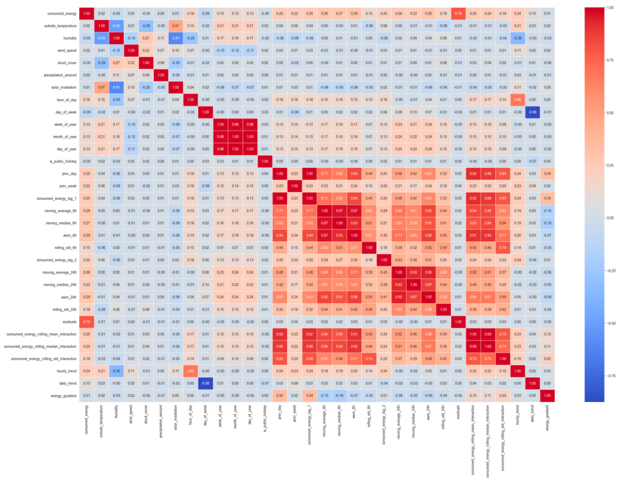
For feature selection, we used the correlation matrix. Figure 3 shows the correlation matrix for total energy production prediction, but a similar matrix was determined for all sources of energy data. We computed the correlation coefficients between all pairs of features and used them to identify features strongly related to each other. The pairs of features holding high correlation coefficients may have redundant information in the prediction process. We identified pairs with a strong positive correlation (represented by the dark red color) and others with a strong negative correlation (represented by the dark blue color). For energy production, strong positive correlations are identified among current energy values and previous values (i.e., day, week), statistical and interaction features. Moreover, temperature and solar irradiation show a strong correlation with the produced energy. Strongly negative correlations are shown between humidity and the quantity of energy generated. To reduce redundancy in our model, we selected only features with high correlation with the energy values, while the features with low correlation coefficients were discarded, not being useful in energy prediction. Even though the correlation scores between temporal features and the energy values are low, we decided to keep them in the training process to preserve a certain degree of order. We decided to keep only features with correlation scores higher than 0.25 or lower than −0.25 to the energy values.

Figure 3. The correlation matrix for total energy production.

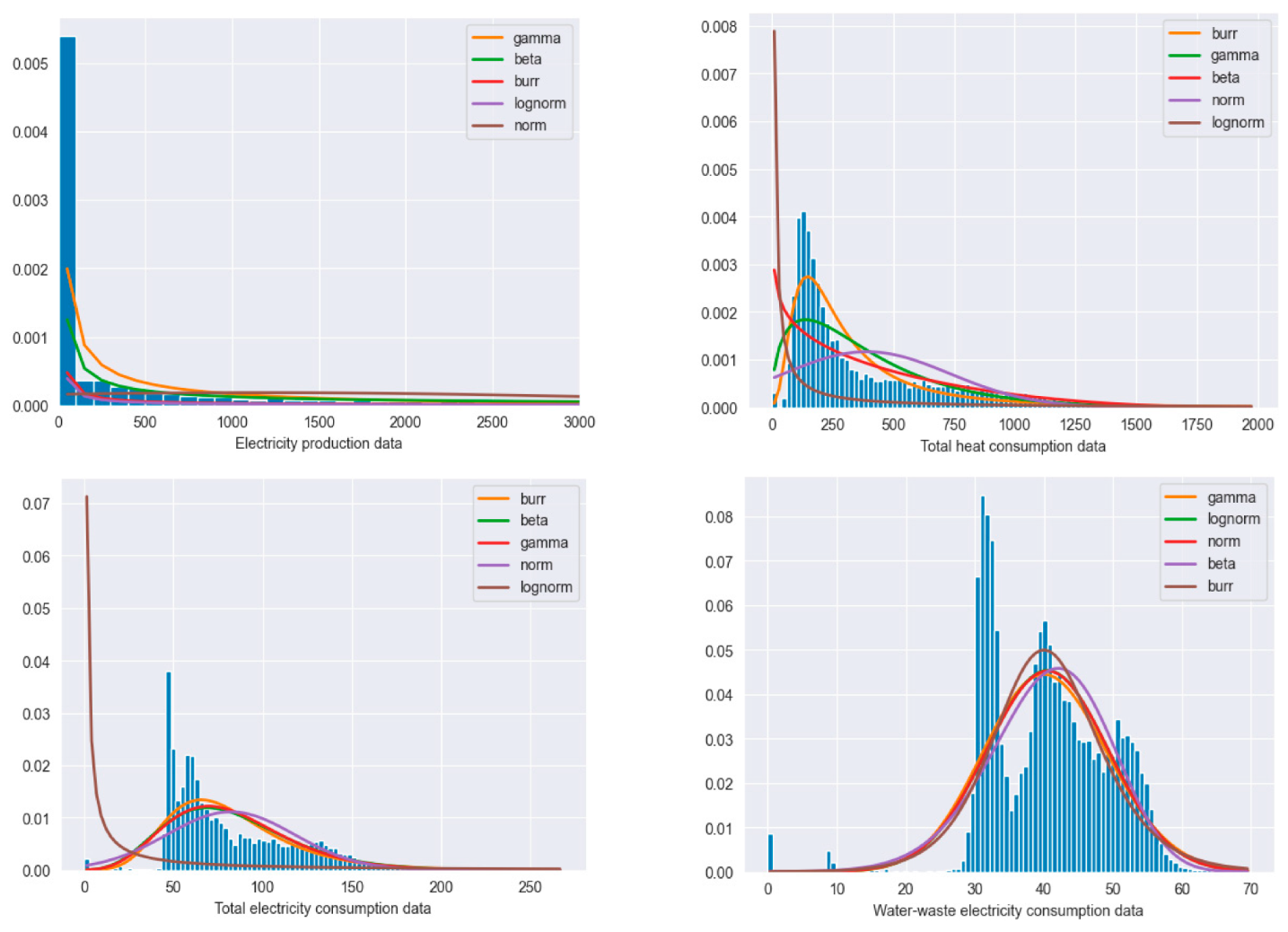
To gain a more insightful look into the different energy data used for the MLP model training and to help us choose the appropriate statistical methods for modeling the data (see Figure 4), we analyzed which of the following distributions best suited our data: normal, gamma, beta, log-normal, and Burr. The least squares estimation statistical technique was used to determine the energy data distribution models. The main principle underlying least squares estimation for distribution fitting is to minimize the sum of the squared errors between the observed data and the fitted distribution’s projected values [42]. In the case of energy production data (see Figure 4 top left), a gamma distribution is the best fit. The data appear to be heavily skewed, with a very long right-tail, values around 0, which is the common value for nighttime. The total electricity consumption follows a Burr distribution model (see Figure 4 top right). The distribution is more left-peaked around the value 50 and right-skewed with a heavier tail on the right side. It reflects that the data can underly more complex trends and patterns. The heat demand data follow a Burr distribution as well (Figure 4 bottom left), with data being right-skewed with a heavy tail on the right side, meaning that extreme values are present in the data that can have an important impact on the training process. Finally, wastewater treatment energy demand data distribution follows the pattern of a gamma distribution (see Figure 4 bottom right).

Figure 4. Distribution models fitting the district-level energy data sources.

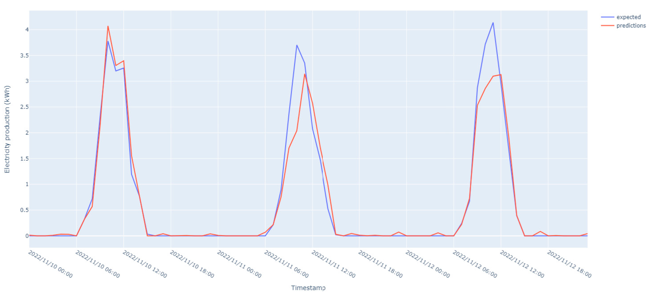
The results of the energy prediction models for different data sources are presented in the following figures, where the blue line represents the expected values, and the orange line represents the predictions obtained by the models. They offer a visual representation of the accuracy of the models based on the closeness and deviation of the two lines. To assess the accuracy of the prediction, the symmetric mean absolute percentage error (SMAPE) is calculated by summing the absolute difference between the forecast ($F_t$) and anticipated values ($A_t$) divided by the total of the two.

$$SMAPE=\frac{100}{n}{\sum }_{t=1}^n\frac{\left|F_t-A_t\right|}{\left|A_t+F_t\right|/2}$$

(7)

SMAPE is symmetric, which implies that it handles over- and under-predictions equally, in contrast to other error measures. The value of SMAPE is given as a percentage and varies from 0% to 200% and the energy prediction accuracy increases for lower values.

Figure 5 shows that the model trained on electricity production data performs well and is able to capture the patterns and trends in renewable energy generation. However, there is a certain amount of uncertainty in the prediction process caused by the stochastic nature of renewable generation. Possible causes regarding this could be the high weather variability. The local weather conditions heavily influence energy production, which is strongly dependent on the variations in weather conditions such as sunlight, temperature, or humidity. Their localized variations are not always accurately reflected by the weather services APIs that provide data for wider regions. Moreover, it being a data-driven pipeline, it does not consider the physical characteristics and setup of renewable generation infrastructure regarding azimuth, solar inclination, effects of latitude and longitude on solar irradiation, and photovoltaic panel characteristics affecting the amount estimation potential.

Figure 5. Energy production prediction results over 3 days (SMAPE = 5.94).

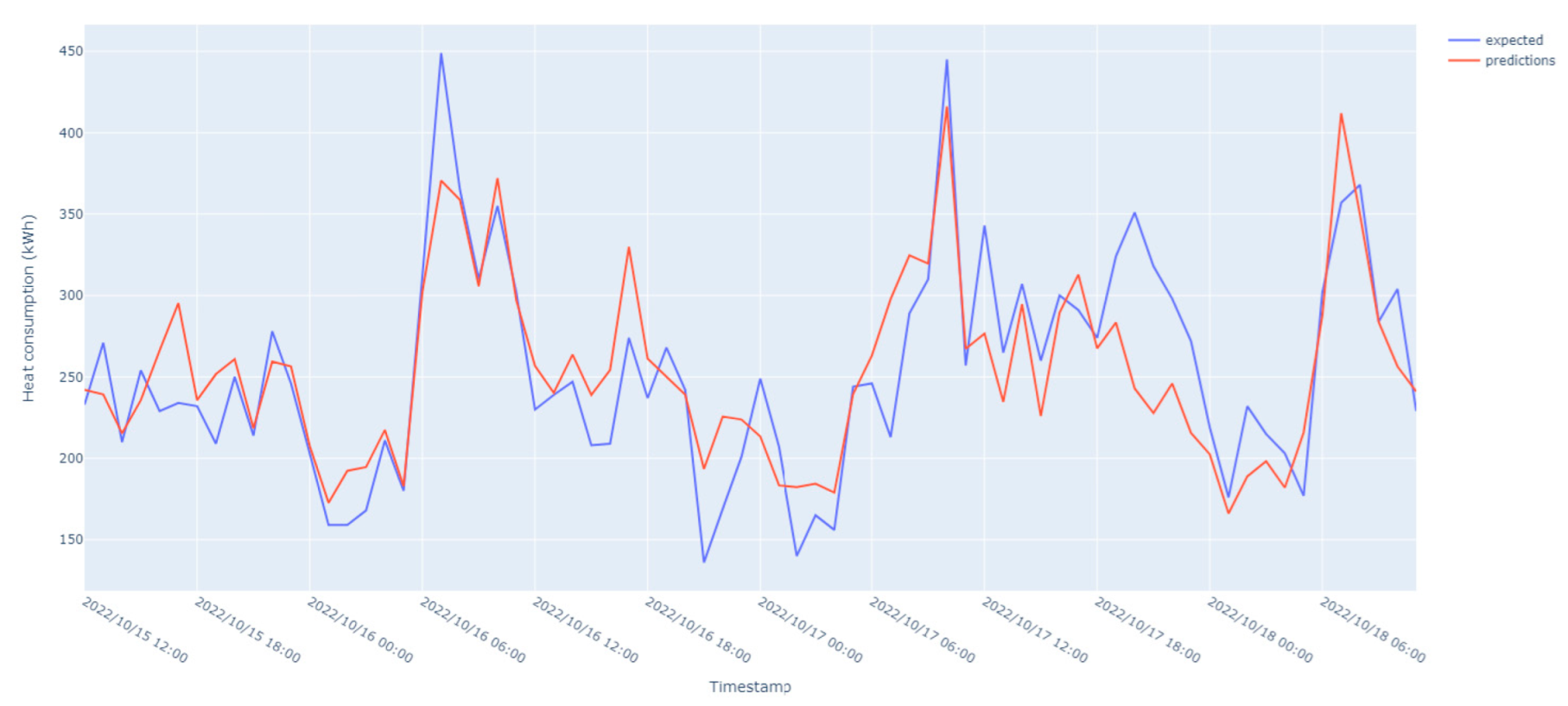
The prediction heat demand results (see Figure 6) show that even though the model captures the trend in data well, there is a variability in performance across different periods of a day that may be generated by several factors, such as changes in resident behavior.

Figure 6. Heat demand prediction results over a three-day period (SMAPE = 11.1%).

The number of people living in the building and their patterns of activity are not used by the model and can significantly influence heat demand, generating a high variability in data. Further investigation is needed to determine the exact factors contributing to the variability in prediction accuracy at different periods of the day. The best predicted periods, which are shown in the figure, demonstrate that the model’s predictions are most accurate during the early morning and early evening hours. The model’s strong performance during these periods suggests that it could be useful for predicting the heat demand in the district during periods of a high peak, which is important for thermal energy management and planning.

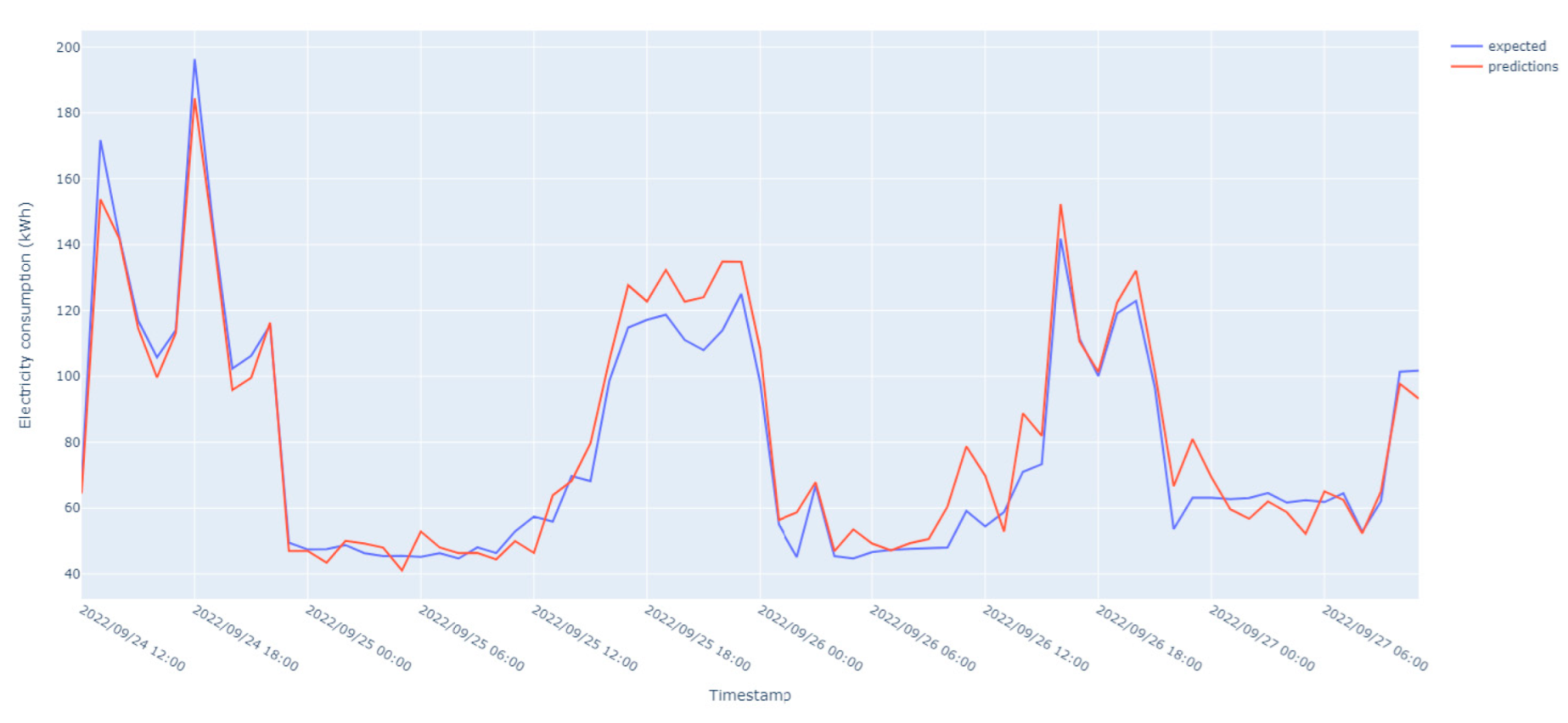
The prediction results for electricity consumption prediction are shown in Figure 7. The trained MLP model performs well, being capable of generalizing and identifying the demand trends. The problem of noise present in the dataset and high variability during the intraday hours need to be assessed in further iterations. This suggests that the model can capture the overall trends in energy demand but may have difficulty predicting the more subtle variations that occur during certain periods, such as sudden surges, or drops in the total energy consumption determined by weather conditions, system malfunctions, or changes in household behavior.

Figure 7. Energy consumption prediction results over a three-day period (SMAPE = 8.32%).

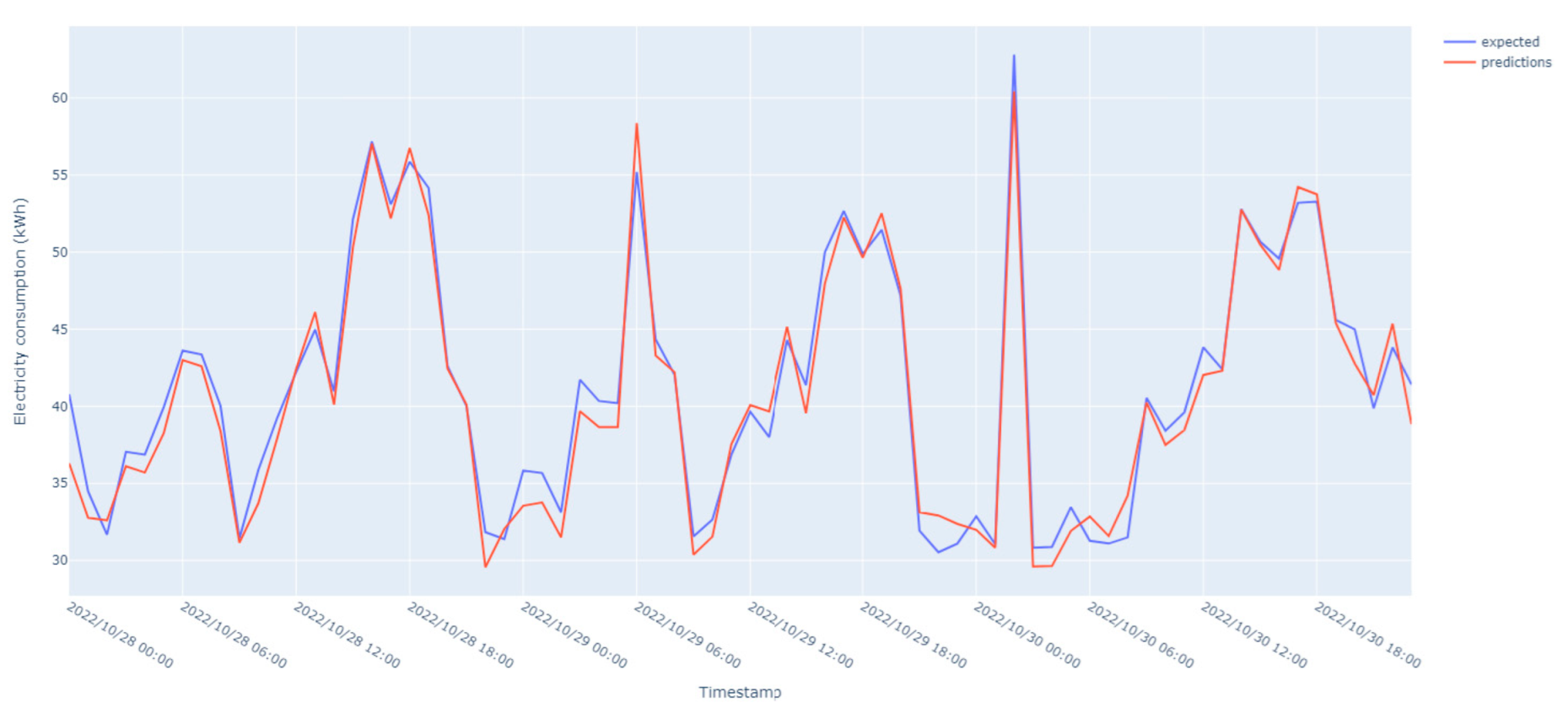
The model trained using wastewater treatment facility data performed better than the others, being helped by the shape of the data, and its value distribution was more compact and had a relatively strong trend component (i.e., steady increase or decrease trend over time).

As can be seen in Figure 8, the dataset exhibits very good performance overall, with great accuracy and precision. Low mean error levels and strong correlation coefficients between anticipated and actual values demonstrate this.

Figure 8. Wastewater electricity consumption predictions over 24 h (SMAPE = 2.65%).

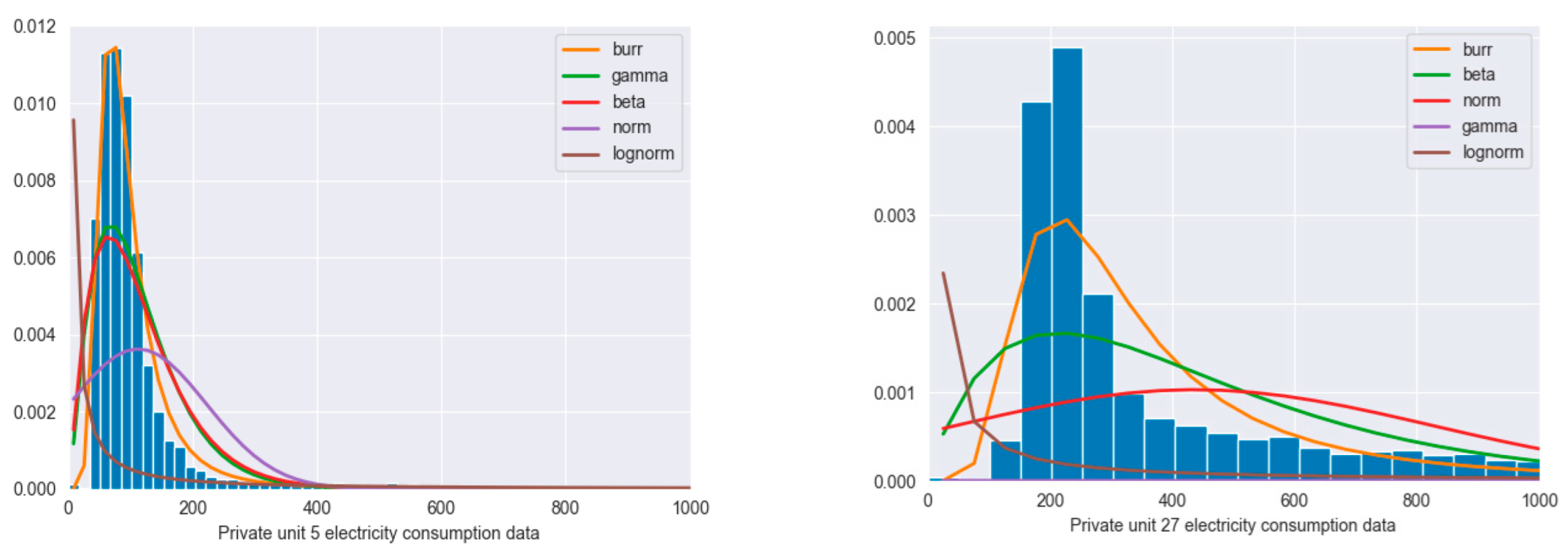
For predicting energy demand for individual units, the MLP model’s accuracy is negatively affected by two factors: the scale of the data and the variability of the data that feature a larger range of variation or fluctuation. Figure 9 shows that the energy data corresponding to the private units follow the Burr distribution. In the case of private unit 5, the data distribution presents moderately skewed data with a peaked shape around the value 100 and a heavy tail to the right that can affect the training process if no outlier detection methods are employed. The data distribution for private unit 27 has a moderately skewed distribution, with a moderate peak around the value 200, with a lighter right-tail, meaning that higher values will not necessarily punish the model’s performance.

Figure 9. Distribution of energy demand data for the private units.

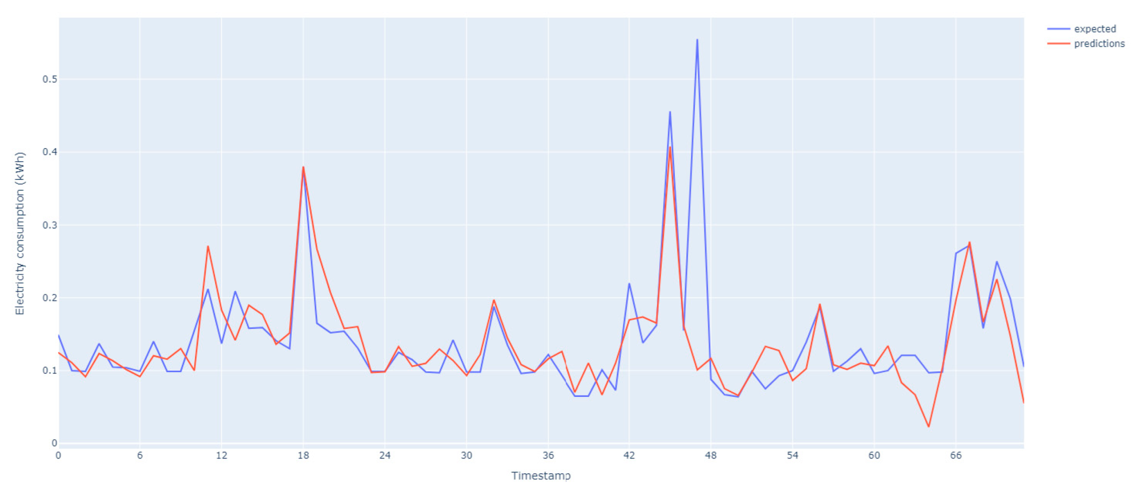
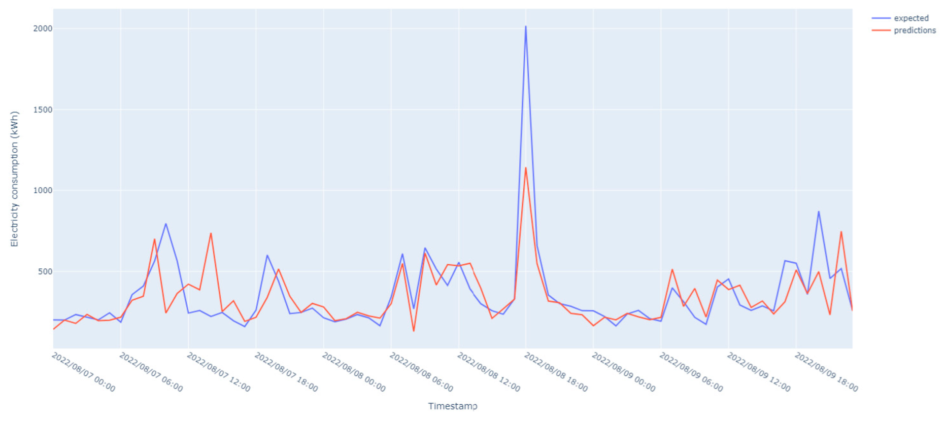
The results of energy forecasting for private units are shown in Figure 10 and Figure 11. The prediction accuracy tends to fluctuate due to numerous variables that impact energy usage in households. These variables, such as the behavior of people and families, can make it difficult for models to accurately predict energy usage levels for individual households. However, the model can still capture the overall trend of consumption patterns and provide valuable insights into energy use.

Figure 10. Private unit 5 electricity consumption predictions for three days.

Figure 11. Private unit 27 electricity consumption for three days.

The model tested on these datasets aimed to forecast energy consumption levels for individual households by analyzing historical energy use data. The model did not consider variables such as the number of people living in a home, their daily schedules, energy-saving practices, and the use of energy-intensive gadgets, and the model struggled to accurately predict energy usage levels for individual households due to the variability of these variables between households.

The data over the year 2022 are noisy and with variable behavior, with sudden surges and drops in energy consumption over short and very short periods. Despite these challenges, the model was able to capture the overall trend of energy consumption patterns for households. The models performed well, especially during the early morning hours, struggling to accurately forecast energy consumption during afternoon and evening hours. Moreover, during periods of constant energy consumption, the model did not perform well and could not capture the constant value, even though the resulting error was small.

However, SMAPE is known to be more sensitive to smaller values that are closer to zero, which are heavily penalized. For the private units their monitored energy values are often below 0.5, thus SMAPE is not the best metric to use for measuring prediction accuracy in their case. To provide a more thorough assessment (see Table 5) of the forecast accuracy, we used Mean Absolute Error (MAE) and Mean Absolute Scaled Error (MASE). MASE was selected because it is scale-invariant, robust to seasonality, and suitable for intermittent demand (for load datasets with multiple values closer to zero. MASE normalizes the error by a measure of the variability of the historical data. Using these metrics, it can be seen how the model will generalize in comparison with a baseline naive model.

Table 5. Accuracy results of the energy prediction process.

Data Sources	MAE	MASE
Total Electricity Production	1.6	5 × 10−4
Total Electricity Consumption	1.64	7 × 10−5
Total Heat Demand	0.03	3 × 10−4
Wastewater Treatment Electricity Consumption	3.27	2.5 × 10−3
Private Unit 5	0.036	1.9 × 10−4
Private Unit 27	0.18	4 × 10−4

5. Conclusions

In this paper, we developed a data-driven pipeline based on ML to forecast the electricity and thermal demand of buildings and energy assets. We covered all pipeline activities from processing the energy data, model integration, data enrichment and features engineering, and MLP model training. The pipeline was designed in a way that is flexible and adaptable to different types of sensors and neural network topologies, allowing the integration of weather data, and with new features engineered by fusing the energy data with statistical models to capture nonlinear relations in energy usage.

The results obtained for the energy data and assets of a city district in Belgium show the effectiveness of a ML pipeline for accurately predicting electricity and heat demand. The data-driven approach and incorporation of various statistical and interaction features enabled the detection of complex patterns and trends in energy usage. Moreover, it successfully handles large amounts of energy data from different types of sensors with heterogeneous formats offering good generalization features without considering the characteristics of the energy assets behind the meter.

As future work, we plan to increase the accuracy of the prediction by incorporating in the pipeline new features related to the spatial and temporal dependencies in data and physical characteristics of the energy assets for a secondary path for physics-informed ML-based predictions. In this way, the district or buildings level management services that collect cross-sectorial big data information can first use the data-driven pipeline for assessing the demand and flexibility on wider scales. Afterwards, they may take the alternative path of using digital models to accurately predict energy demand by combining a physics-based understanding of energy assets with data-driven insights. The services will be able to leverage the strengths of each to create a more accurate and comprehensive understanding of energy demand, facilitating AI-based decision-making related to district-level resources management and strategies using variable time frames with improved levels of accuracy.