Article

Development of an IRMO-BPNN Based Single Pile Ultimate Axial Bearing Capacity Prediction Model

Department of Civil Engineering, Central South University, Changsha 410075, China
*
Author to whom correspondence should be addressed.
Buildings 2023, 13(5), 1297; https://doi.org/10.3390/buildings13051297
Submission received: 14 April 2023 / Revised: 10 May 2023 / Accepted: 12 May 2023 / Published: 16 May 2023
(This article belongs to the Special Issue Advanced Materials and Novel Technique in Civil Engineering)

Abstract

:
The ultimate axial bearing capacity (UABC) of a single pile is an important parameter in pile design. BP neural network (BPNN) has a strong nonlinear mapping ability and can effectively predict the UABC of a single pile. However, frequent immersion in unstable search results with local vibration leads BPNN to a less usable solution. The weights and biases of the BPNN model are optimized using the improved radial movement optimization (IRMO) algorithm in this study, and a new method named the IRMO-BP neural network (IRMO-BPNN) is proposed to predict the UABC of a single pile. The IRMO-BPNN model was developed from a database of 196 static load test (SLT) samples, and model hyper-parameter analysis was carried out to determine the optimal number of hidden nodes, population size, and the number of iterations. The prediction accuracy and stability of the IRMO-BPNN model are verified by comparing it with the GA-based ANN model, ANFIS-GMDH-PSO model, and RBFANN model. The results show that the IRMO-BPNN model can accurately predict the UABC of a single pile and improves the situation that the BPNN model is easy to fall into local optimal values and its search results are unstable. The IRMO-BPNN model has significant advantages over other models.

1. Introduction

A pile is a foundation form of high bearing capacity, wide applicability, and a long history of utilization. As infrastructure construction continuously develops, piles are widely used in high-rise buildings, ports, and bridge engineering. The ultimate axial bearing capacity (UABC) of a single pile is significant in pile design since it is directly related to the safety and economy of engineering construction [1]. Over the years, many scholars have investigated the UABC of single piles using in situ tests [2,3,4], theoretical analysis [5,6,7], and numerical simulation [8,9]. The actual pile–soil interactions are usually simplified and assumed in the theoretical analysis and numerical simulation methods. Therefore, their calculation accuracy often cannot satisfy the requirements. The static load test (SLT) is the most direct and reliable method for determining a pile’s UABC, but it is time and cost-consuming. As a result, an alternative method for predicting the UABC of a single pile that can satisfy calculation accuracy with actual pile-soil interactions is required.
As a practical, feasible, and fast method to solve engineering problems, machine learning provides an approximate solution for predicting the UABC of a single pile and can consider various influencing factors. The artificial intelligence algorithms used to predict the UABC of a single pile include, for example, the grey predicted model, the artificial neural network (ANN), and the support vector machine. Among them, ANN has been adopted by many scholars due to its strong nonlinear mapping ability and fault tolerance. Based on the dynamic test data, Chan et al. [10], Lee et al. [11], and Goh [12] developed the BP neural network (BPNN) to determine the UABC of driven piles. Benali and Nechnech used ANN to predict the UABC of purely coherent soils under weightlessness [13]. Benali et al. combined ANN and principal component analysis and used back-propagation multilayer perceptron with Bayesian regularization to predict the UABC [14].
However, the traditional ANN has the disadvantages of easily falling into local minima, having a slow learning rate, slow convergence rate, over-fitting, and poor stability [15,16]. Hence, many scholars combined high-performance optimization algorithms with ANN to improve its performance. Momeni et al. [17] predicted the UABC of driven piles using ANN based on a genetic algorithm (GA-based ANN). The findings demonstrated that the GA-based ANN model is not only a practical and effective tool but also performs better in terms of accuracy than the conventional ANN model. The most important parameters discovered by performing a sensitivity analysis on the input variables are the hammer weight and pile geometrical characteristics. Similarly, Armaghani et al. [18] applied ANN optimized by particle swarm optimization (PSO) algorithm to predict 132 rock-socketed piles’ UABC. The coefficient of determination (R2) of the PSO-ANN model is higher than that of the ANN model. In order to estimate the UABC of driven piles in cohesionless soils, Moayedi and Jahed Armaghani [16] developed an ANN optimized by the imperialist competition algorithm (ICA). By comparing the R2, root mean square error (RMSE), and variance account for (VAF) of the ICA-ANN model and ANN model, it is concluded that the ICA-ANN model has a faster convergence rate and higher accuracy. For the purpose of predicting the UABC of driven and drilled piles, Benali et al. [19] created a TLBO-ANN model using the teaching-learning-based optimization (TLBO) technique. The prediction accuracy and generalization performance of the TLBO-ANN model are better than the BPNN model. Among these hybrid algorithms, the global optimization algorithm is used to enhance prediction accuracy and convergence speed and prevent the ANN model from entering the local minimum. However, there is a lack of introduction on how ANN avoids over-fitting and how to improve the search stability, and they were only analyzed in comparison with ANNs, not with other hybrid algorithms.
The purpose of this article is to introduce the improved radial movement optimization (IRMO) [20,21] into the field of pile foundation engineering and combine the IRMO algorithm with BPNN to establish a new method called IRMO-BP neural network (IRMO-BPNN) for predicting the UABC of a single pile. The IRMO-BPNN model is developed based on 196 SLT data and compared with the GA-based ANN model, RBFANN model, and ANFIS-GMDH-PSO model to verify its superiority. Section 2 introduces the concepts of the IRMO algorithm and BPNN and analyses the advantages and disadvantages of both. Section 3 illustrates the synergistic effects of the IRMO algorithm and BPNN and the implementation of IRMO-BPNN. Section 4 develops the IRMO-BPNN model and conducts sensitivity analysis on its hyper-parameters based on 196 data sets. Section 5 firstly analyses the prediction results of IRMO-BPNN and its superiority over BPNN, and secondly compares and discusses the prediction performance of IRMO-BPNN with other hybrid algorithms. The conclusion of this study is presented in Section 6.

2. IRMO Algorithm and BPNN

2.1. IRMO Algorithm

The improved radial movement optimization (IRMO) is a global optimization algorithm developed based on the radial movement algorithm (RMO) [22]. It benefits from having a quick convergence rate, a short storage area, a clear data structure, and strong stability.
The RMO algorithm relies on the continuous generation and updating of particle positions within the solution range to find the optimum solution. First, the initial particle groups are randomly generated within the solution range, and the initial optimal position is determined by comparing the function values of each particle, which is defined as the initial center. In each subsequent generation, particles are regenerated near the center position. The contemporary optimal position is the perfect position for each generation, and the global optimal position is the ideal position for all generations. The center position moves with the contemporary optimal position and the global optimal position. Once it reaches the final generation, the solution range converges to a specific point, which is the global optimal position. Figure 1 is a diagram of the RMO algorithm center position movement.
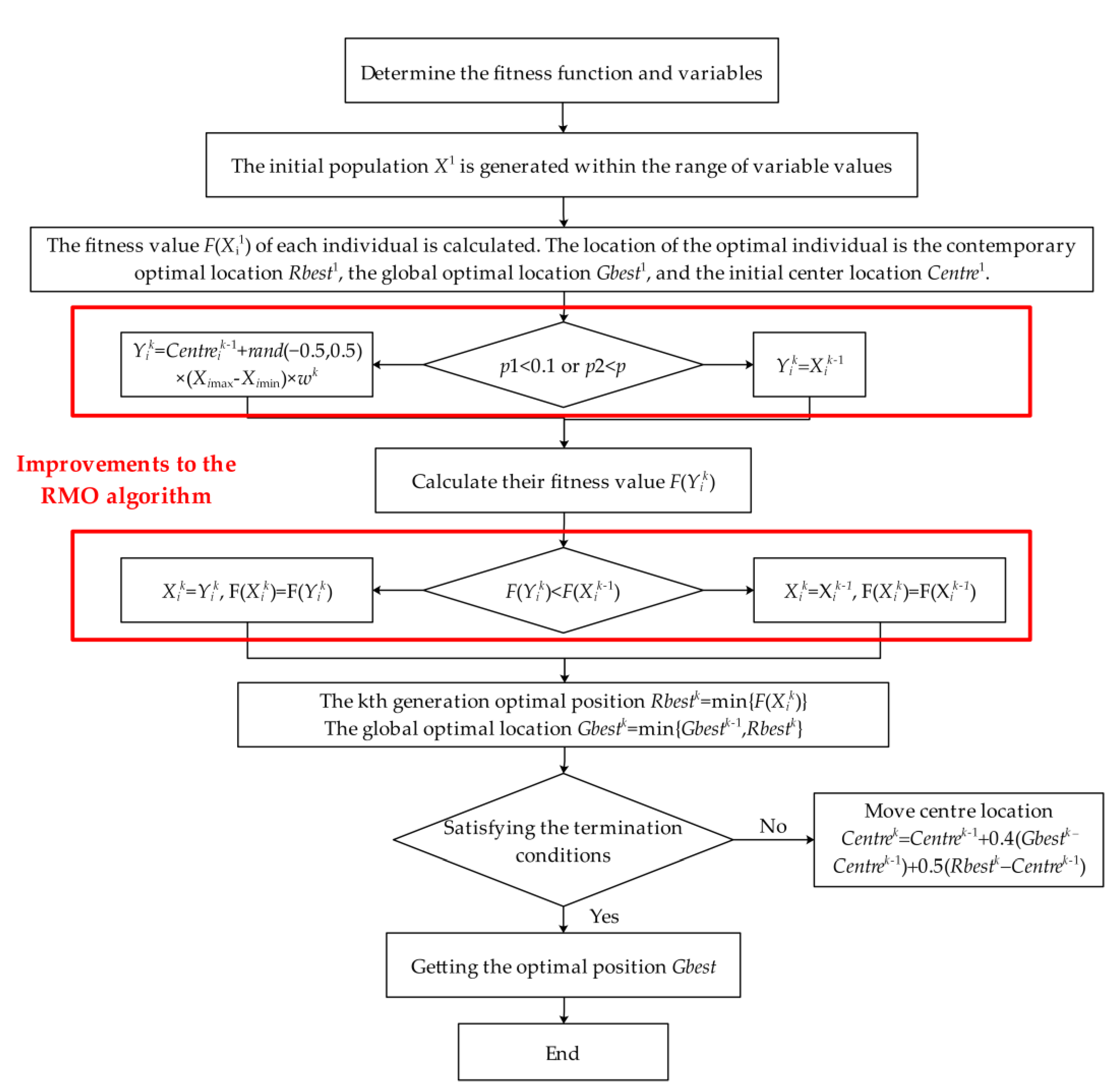
The RMO algorithm generates particles iteratively, but excessive reliance on the center position causes the particles to lose information from earlier generations and produce random outputs. However, the IRMO algorithm generates pre-position points and determines whether to update the position information by comparing the function values of pre-positions with the function values of the previous particles. Moreover, there are two ways to generate pre-position points; one is dependent on the center position, and the other is inherited from the previous generation of particle information. How a particle is generated is determined by two random numbers, p1 and p2. Through the above improvement, the self-feedback of particles can be improved via the IRMO algorithm, allowing the particle swarm to inherit the superior knowledge of its own particles. While the accuracy of the result can be guaranteed, the algorithm’s stability can be significantly increased. Figure 2 shows the flowchart of the IRMO algorithm.
The population generation in the IRMO algorithm iteration process depends on the value range of the particle variables, and the size of the variable value range is determined by the inertia weight w. As w increases, the algorithm gets better at global search and worse at local search. This article employs a basic linear decreasing form of w to balance global and local searches. The nonlinear decreasing form of w has yet to be explored. The IRMO algorithm yet has much potential for application in civil engineering and is currently only used for the calculation of the ultimate bearing capacity of foundation [21], the optimization search of the critical sliding surface of two-dimensional slope [23], and the prediction of the UABC of single pile mentioned in this article.

2.2. BPNN

The BPNN [11] is a multilayer feed-forward neural network based on an error back propagation (BP) algorithm. It is widely used in engineering because of its ability to realize any nonlinear mapping of input and output [12]. The BPNN is composed of an input layer, one or more hidden layers, and an output layer; each layer is composed of several nodes (neurons), and the layers are connected by weights and biases [17].
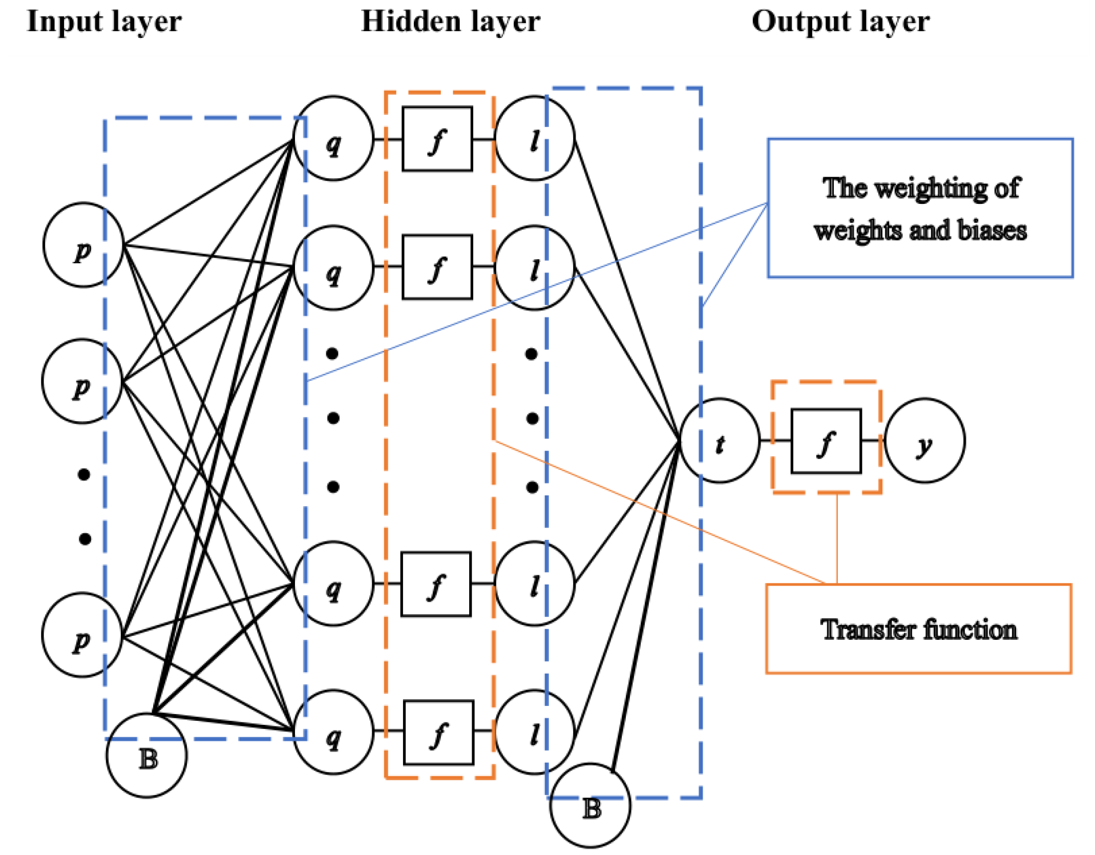
The BPNN model comprises an input layer, a hidden layer, and an output layer. Each layer is composed of several nodes (neurons), and the signal is transmitted to the nodes of the next layer through weight and bias, and then the nonlinear transformation of the signal is realized through the activation function. Each node goes through a similar process until the output is generated. The generated output is compared with the target output, and the error is calculated. If the error does not meet the accuracy requirement, the network will be back-propagated, modifying the weights and biases to reduce the error until the accuracy requirement is met. Figure 3 shows a typical BPNN architecture.
The BPNN can approximate any function and has a strong nonlinear mapping ability; however, its disadvantages of easily falling into local minima [17] and unstable search results cannot be ignored. Moreover, a BPNN needs to artificially set parameters such as the number of hidden layers, the number of hidden nodes, tolerance, learning rate, and the maximum number of iterations. The output will have a great discrepancy with the changed hyper-parameters. Furthermore, considering the sample data provides the network with all of the knowledge, the representativeness of the sample and the completeness of the information impact the correctness of the assessment results to a great extent. As a result, the network can only guarantee its prediction accuracy and generalization ability if it obtains complete and accurate data.

3. IRMO-BPNN

3.1. The Proposed IRMO-BPNN

With a large amount of data, BPNN on its own can achieve a mapping relationship of nonlinear functions and hence prediction. However, it is easy to fall into local minima, slow to converge, and has unstable search results. The IRMO algorithm on its own can only optimize for specific problems if the fitness function is known. In contrast, when the IRMO algorithm is combined with BPNN, good predictions can be achieved with only data available. Moreover, it improves the prediction accuracy, increases the convergence speed, and ensures the stability of the results while not falling into a local optimum.
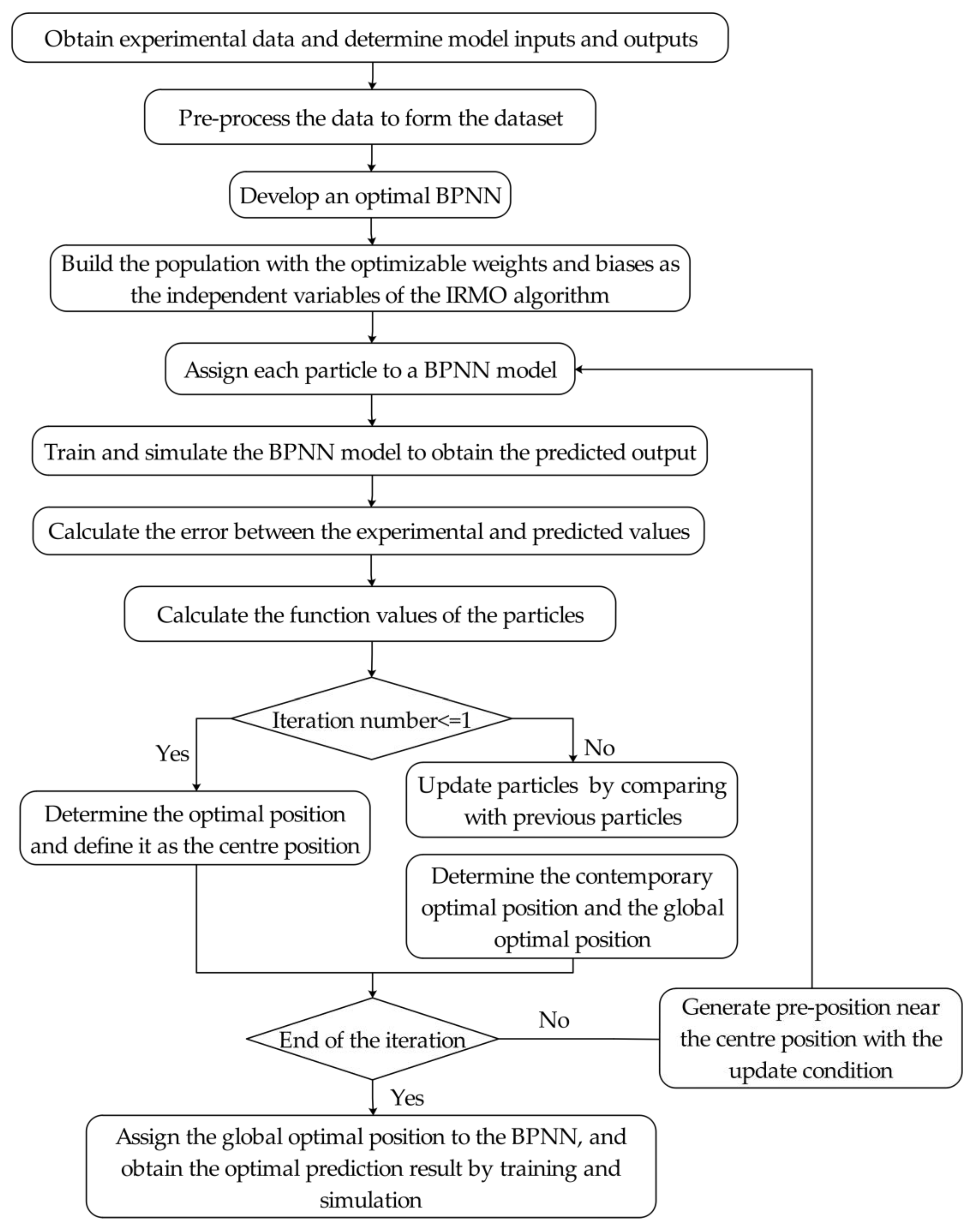
Based on the combination of a BPNN and the IRMO algorithm, a new ANN called IRMO-BPNN is proposed in this article, and it is used to predict the UABC of a single pile. IRMO-BPNN takes the weights and biases of BPNN as the independent variables of the IRMO algorithm and the performance function of BPNN as the objective function of the IRMO algorithm to realize the optimization of the weights and biases of BPNN by the IRMO algorithm. After the optimization, the optimal weights and biases are assigned to the BPNN model, and the BPNN model is trained and simulated to obtain the optimal predicted UABC of a single pile.
If adequate, relevant data is collected, IRMO-BPNN may be utilized to estimate not just the UABC of a single pile but also the ultimate bearing capacity of pile groups and foundations. It is important to keep in mind that the sample data must be representative and thorough, and the data must include both the output and the input factors that have a significant impact on the output. Although IRMO-BPNN’s prediction performance is superior to BPNN’s, it still depends on the hyper-parameters. Therefore, when developing the model, suitable hyper-parameters must be used.

3.2. Implementation Steps of the IRMO-BPNN

The IRMO-BPNN is a combination of the BP neural network and IRMO algorithm, and its flow chart is shown in Figure 4.
First, a BP neural network needs to be developed. In the first step, as the dataset is very important for the neural network, a large amount of experimental data needs to be acquired before the network can be developed. In the second step, the experimental data is pre-processed to form a dataset, and the dataset is divided into a training set, a validation set, and a test set. The BP neural network is trained and simulated using the dataset in the third step, and the prediction output is obtained.
Second, the improved radial movement algorithm is used to optimize the built-in weights and biases of BPNN. On the one hand, the built-in weights and biases of BPNN should be used as the particle information of the IRMO algorithm to establish the population. The total number M of weights and biases is calculated according to Equation (1), where I and J are the number of nodes in the input layer and hidden layer, respectively, and the number of nodes in the output layer is 1. Then, because the weights and biases are small random nonzero values, the upper Xmax,j and lower Xmin,j limits of variables (weights and biases) are set to 0.5 and −0.5, as shown in Equations (2) and (3).
M = I   ×   J + J   ×   1 + I + J
X max = [ 0 . 5 0 . 5 0 . 5 ] 1 × M
X min = [ 0 . 5 0 . 5 0 . 5 ] 1 × M
On the other hand, in order to find the optimal weights and biases to increase the predictive performance of the BPNN, the performance function mean square error (MSE) of the BPNN is taken as the objective function of the IRMO-BP algorithm. The specific formula is as follows:
F ( · ) = 1 L i = 1 L ( y i   t i ) 2
The performance function is obtained by running the BPNN developed above. In the formula, L is the number of samples, ti is the predicted value of the i-th sample, and yi is the experimental value of the i-th sample.

4. Development of an IRMO-BPNN Model

4.1. The Inputs and Outputs of the Model

The UABC of a single pile is the maximum load before the pile reaches the collapse state under vertical load, or the deformation is not suitable for continuous bearing. Li et al. [24], Hamed et al. [9], Gu et al. [25], and Chen et al. [26] analyzed the bearing performance and the influencing factors of a single pile under axial load. The results showed that the factor affecting the UABC of a single pile includes the geometric size of the pile and the properties of the soil at the side and tip of the pile.
In this article, pile length L, pile diameter D, the weighted average value (sum) of the cohesion c ¯ and internal friction angle φ ¯ of the soil around the pile and the ultimate tip resistance standard value qpk of the pile are selected as the model’s input variables. The UABC Qu is selected as the output variable of the model.

4.2. Data Collection and Pre-Processing

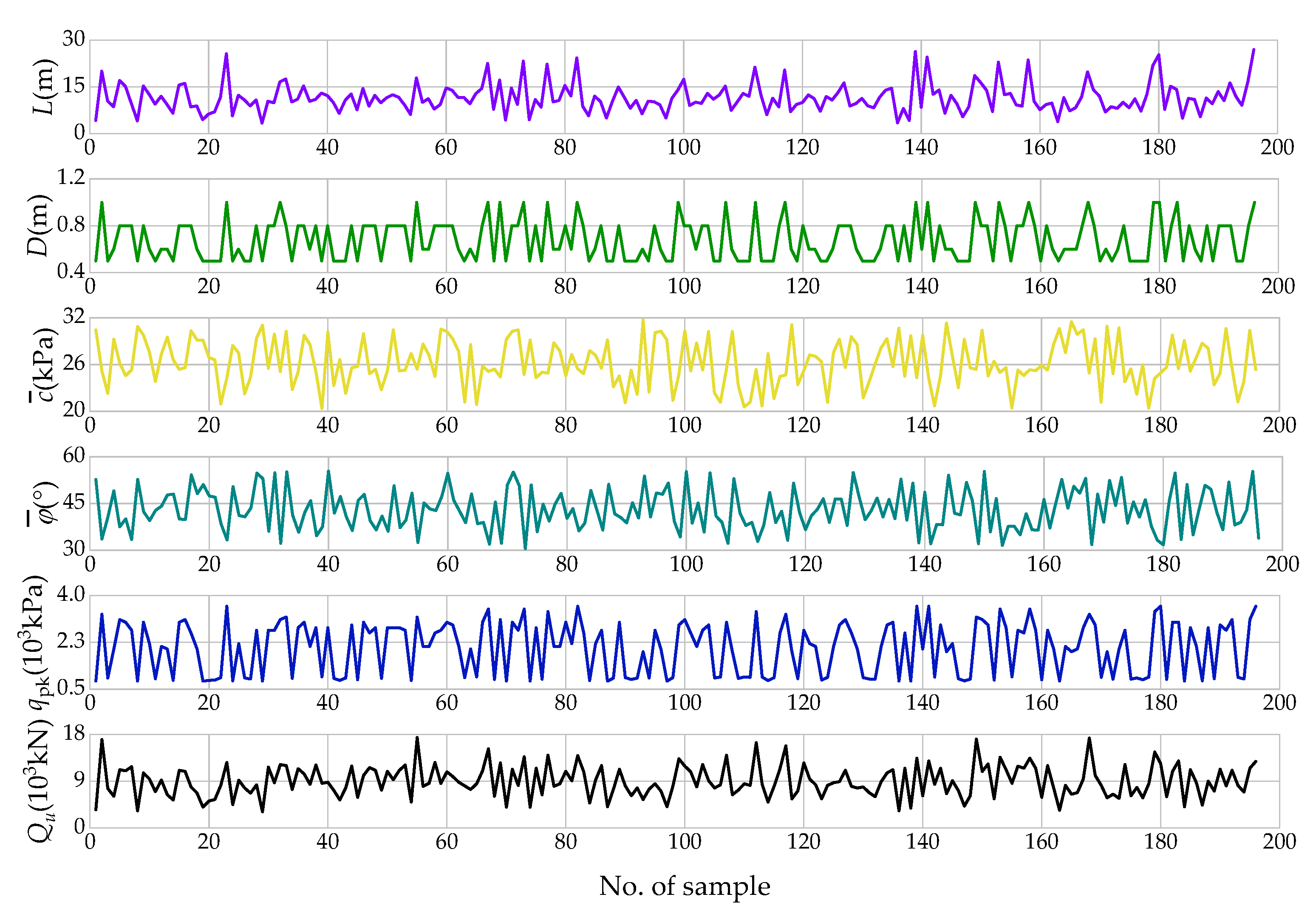
This article collects data on 196 bored piles in Chenzhou, Hunan Province, including the physical and mechanical properties of soil, the geometric size of piles, and the static load test report of piles. Figure 5 shows the indicators and UABC of each pile. The range of L is from 3.4 to 26.9 m, the range of D is from 0.5 to 1.0 m, the c ¯ is from 5.54 to 25.36 kPa, the φ ¯ is from 20.38 to 31.72°, the qpk is from 800 to 3700 kPa, and the UABC is from 3100 to 17,400 kN. The c ¯ and φ ¯ were obtained from the cohesion and the internal friction angle of the soil layer around the pile by a weighted average of the thicknesses, respectively. The qpk was obtained by consulting the Technical Code for Building Pile Foundations (JGJ 94-2008) [27]. The UABC was obtained by static load tests carried out by different researchers.
It is noted that this article only collected some data on bored piles in Chenzhou, Hunan, so the model developed is only applicable to predict the UABC of bored piles in Chenzhou or with engineering geological conditions similar to those in Chenzhou. If the reader wishes to predict the UABC of a single pile in other areas or other geological conditions, this can also be achieved by replacing the data set.
To improve the accuracy of model prediction, the 196 samples collected are processed as follows:

4.2.1. Outlier Processing

In statistical data analysis, outliers, such as abnormal data, will lead to the incorrect estimation of parameters and affect the analysis results. Therefore, it is necessary to filter the outliers in the original data set before analyzing the data. The Mahalanobis distance method [28] was used to test the outliers. The chi-square statistic with 5 degrees of freedom and a 0.005 significance index is 16.75 in this study; that is, the samples with Mahalanobis distance exceeding 16.75 can be determined as outliers. The maximum Mahalanobis distance in 196 samples is 13.58 according to the calculation results, wherein 13.58 < 16.75, which indicates that there is no outlier in the data adopted in this study.

4.2.2. Partition of Data Sets

The data is often split into a training set and a testing set for ANNs. As the ANN is being trained, the built-in weights are adjusted using the training set, and the ultimate generalization performance of the trained model is assessed using the testing set [13]. However, this dividing method is prone to over-fitting during training. Therefore, this article uses the cross-validation method [29] to evaluate the performance of the model, that is, during the training process, the model performance is preliminarily evaluated in advance by the validation set, and if there is over-fitting, the parameters can be adjusted in time. In this article, the data were divided into a training set (samples 1 to 116), a validation set (samples 116 to 156) and a test set (samples 156 to 196) according to the ratio of 3:1:1. The specific statistics of the data are shown in Table 1.

4.2.3. Data Normalization

In this study, the data are linearly transformed through min-max normalization [12], and the original data are mapped into the interval [0,1] to eliminate the dimension of each variable and speed up the convergence speed.

4.3. Parameter Optimization of the IRMO-BPNN Model

A parametric analysis was carried out to establish the number of hidden layers and hidden nodes, the population size nop, and the number of iterations g in order to create an appropriate IRMO-BPNN model to predict the UABC of a single pile.
It has been demonstrated that BPNN can provide precise approximations to any continuous function with just one hidden layer [12]. Hence, just one hidden layer is required. The IRMO-BPNN model with TANSIG and PURELIN activation functions, a Levenberg–Marquardt training algorithm, and a learning rate of 0.01 was set in advance. Information on the BPNN hyper-parameters and the effect of the hyper-parameters on the model can be found in [10] and will not be repeated in this article.
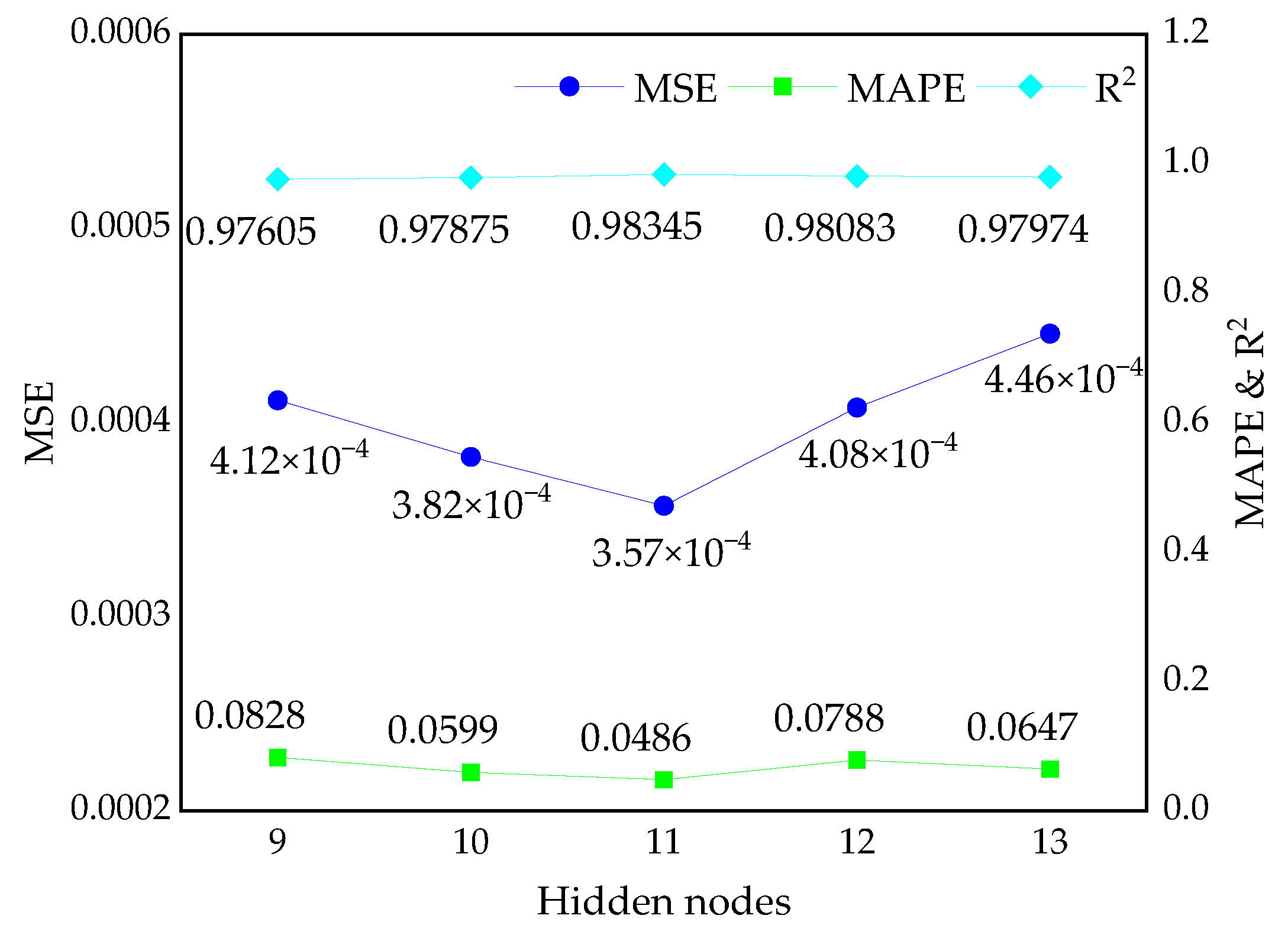
Although some scholars have undertaken extensive studies based on the empirical formula to determine the hidden nodes, it has not yet been turned into a reasonable and reliable theory. It is determined in this article using the conventional trial-and-error method, which costs more to calculate but provides more accurate answers. As shown in Figure 6, the performance of IRMO-BPNN models with different hidden nodes was assessed through the statistical parameters of MSE, R2, and mean absolute percentage error (MAPE). These statistical parameters are determined by Equations (4)–(6).
  R 2 = 1 i = 1 N ( y i t i ) 2 i = 1 N ( y i y ¯ ) 2
  MAPE = 1 N I ×   100 %
Small hidden nodes will lead to underfitting. Large hidden nodes may lead to over-fitting and increase the training time of the model. As shown in Figure 6, the IRMO-BPNN model with 11 hidden nodes has the best prediction performance, with an MSE of 0.00036, R2 of 0.98345, and MAPE of 4.86%.
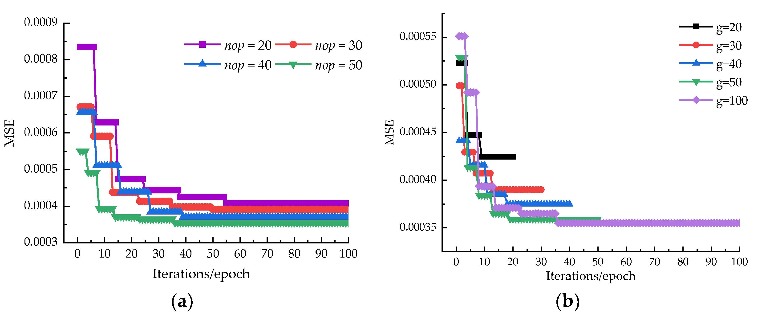
The number of iterations g and the population size nop must be determined once the best number of hidden nodes has been chosen. The model with 11 hidden nodes is used to analyze the effect of g and nop on the model performance. Table 2 shows the performance of models with different g and nop values, where the calculation formulas of the RMSE and VAF are shown in Equations (7) and (8).
  RMSE = i = 1 N ( y i t i ) 2 N
  VAF = [ 1   var ( y t ) var ( y ) ]   ×   100
When nop and g are small, not enough position points are captured, resulting in the model not finding the global optimum. As nop and g rise, the R and VAF, which measure the correlation between the model’s predicted and desired outputs, increase while the MSE, RMSE, and MAPE, which measure the model’s error performance, decrease. When nop is 50 and g is 100, the model has reached a steady state, with a MAPE of 4.86%, an MSE of 0.00036, an RMSE of 0.0190, an R2 of 0.98345, and a VAF of 99.73.
In conclusion, as nop and g increase, the smaller the prediction error of the model, the higher the prediction accuracy, and the faster the convergence rate (as shown in Figure 7). The performance of a model with more g is better when the multiplication of the nop and g is the same, which means that the total number of particles produced is equal. For example, the model with a nop of 40 and g of 50 outperforms the model with a nop of 50 and g of 40. Thus, it is more effective to increase the g of the model to improve the model’s performance.
To sum up, to improve the model’s prediction performance and increase the convergence speed, this article chose g to be 100, nop to be 50, and the number of hidden nodes to be 11.

5. Comparison and Analysis

5.1. Performance of the IRMO-BPNN Model

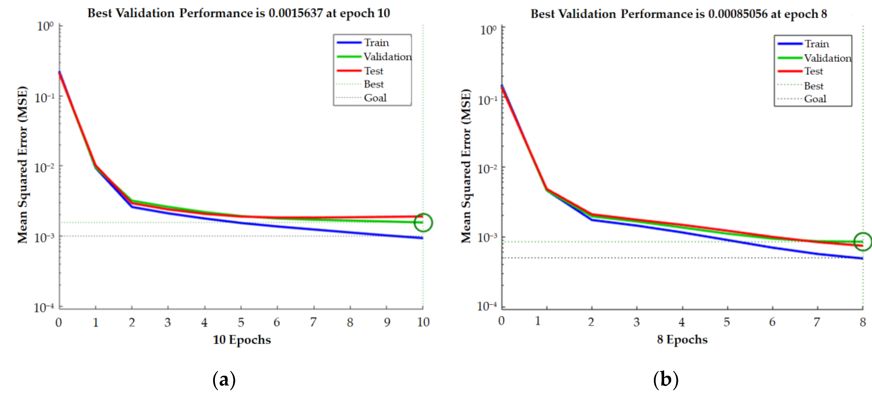
In order to present the superiority of IRMO-BPNN, a BPNN model and an IRMO-BPNN model are developed in this article, where the data set and the hyper-parameters involved in the BPNN model are taken in line with the IRMO-BPNN model. The iteration process of the BPNN model and the BPNN model optimized by the IRMO algorithm is shown in Figure 8. It can be seen that the MSEs of the training set, validation set, and testing set of the two models decrease continuously without over-fitting. Moreover, the BPNN model optimized by the IRMO algorithm is faster to converge, with a prediction accuracy of 10−3 after only 8 iterations.
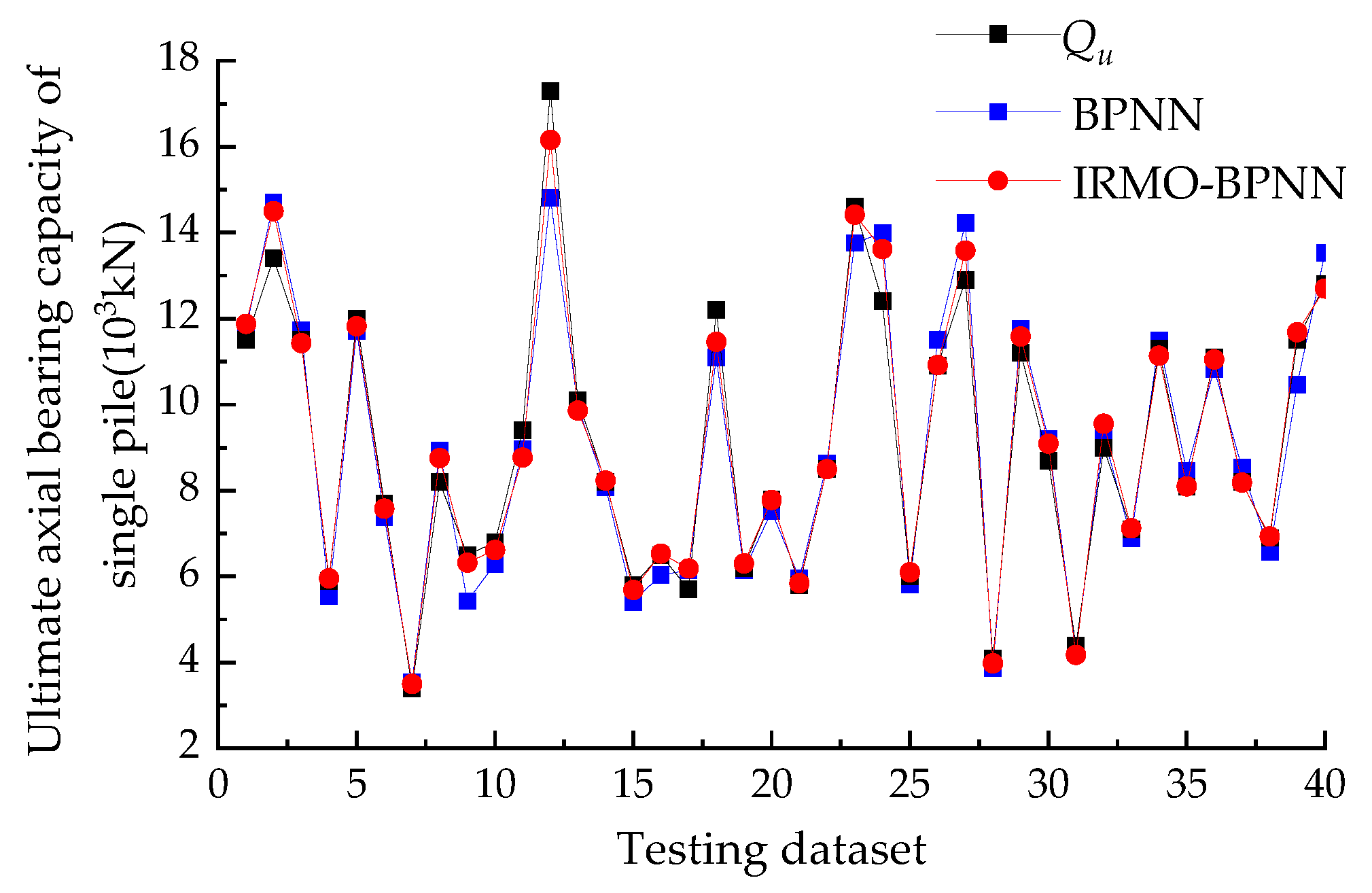
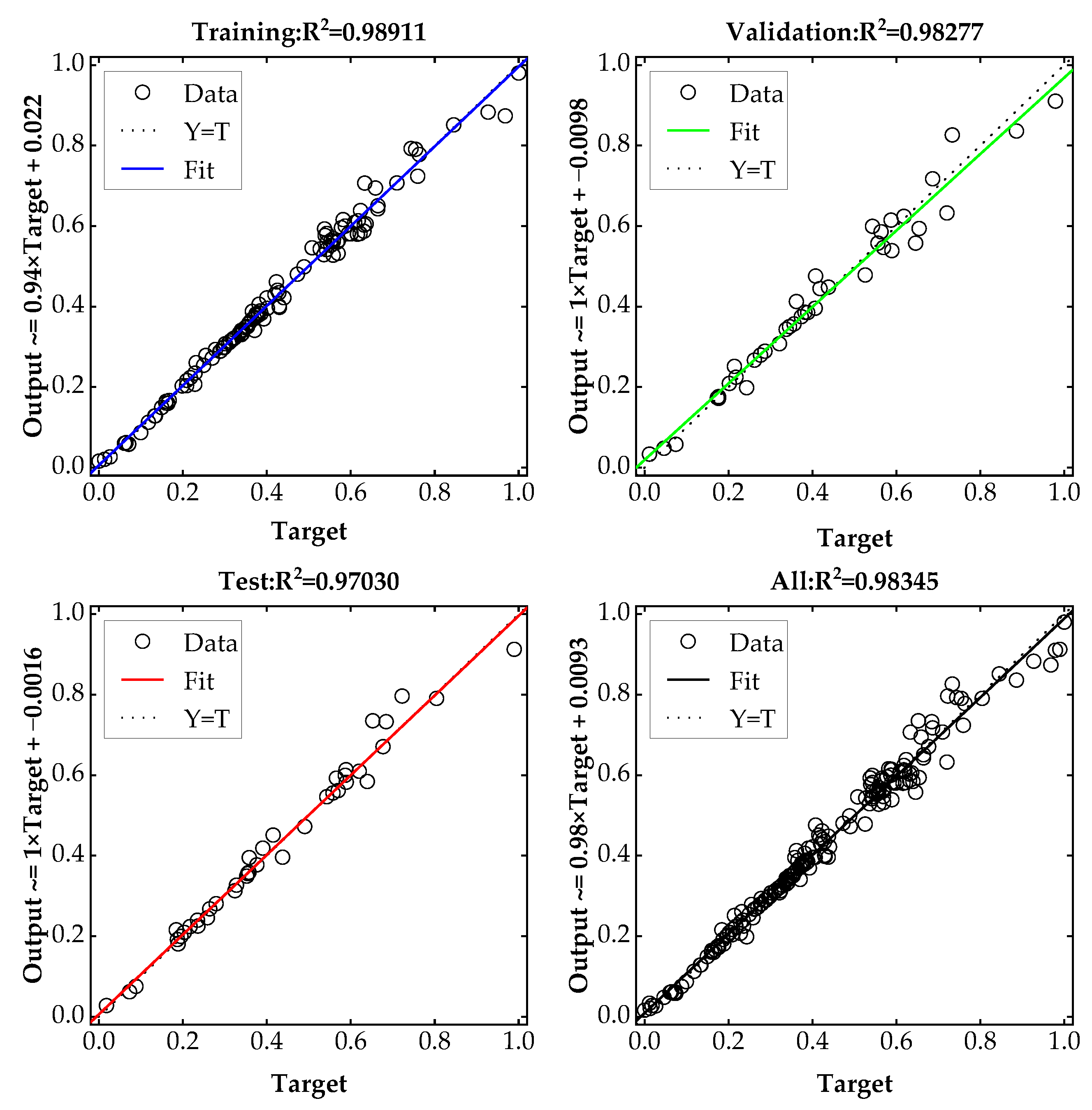
A comparison between the predicted value of the two models and the experimental value Qu of the UABC of a single pile is shown in Figure 9. For the majority of the samples, the BPNN model’s predicted values were near to the experimental values, but in particular samples, the relative error between the predicted and experimental values might reach roughly 20%. The R2 between the predicted and experimental values of the data set reached 0.96, as shown in Figure 10. In contrast, the predicted values of the IRMO-BPNN model overlap almost exactly with the experimental values, with a maximum relative error of 7.16% and a mean relative error of 4.86%, and an R2 of 0.98345 for its data set (as shown in Figure 11). In summary of the analysis above, the IRMO-BPNN model outperforms the BPNN model regarding prediction accuracy and convergence speed.
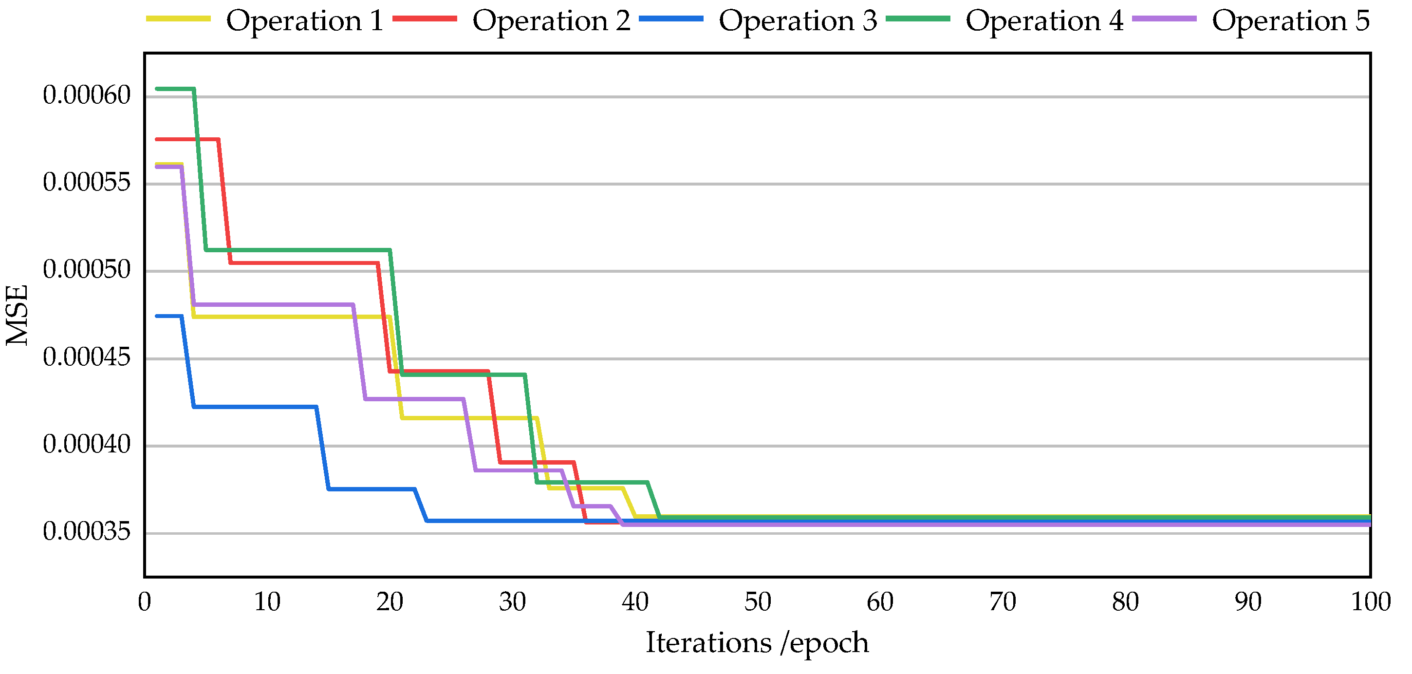
The IRMO-BPNN model with a single hidden layer, TANSIG and PURELIN transfer functions, a learning rate of 0.01, nop of 50, g of 100, and the number of hidden nodes of 11 was repeated 5 times, and the change curve of the MSE during its operation is shown in Figure 12.
Overall, the MSE decreases in a “step-by-step” manner. At the beginning of the iteration, the descent rate is fast. As the iteration continues, the search range continues to shrink, and the MSE decline rate gradually decreases. Finally, around the 50th generation, the global optimum is searched and the MSE tends to be stable. Moreover, it can be seen from the Figure 12 that the best MSE obtained by operating the model with the same parameters five times is roughly the same, indicating that the IRMO-BPNN model has good convergence and stability in the process of global optimization.

5.2. Evaluation and Comparison

In order to further verify the performance of the IRMO-BPNN model, this article will use the model to train and predict the data in the three pieces of literature [17,30,31]. Comparisons are made between the prediction outputs and those obtained using the GA-based ANN model, RBFANN model, and ANFIS-GMDH-PSO model, respectively. The relevant information from the data used in the comparison process is listed in Table 3. Six statistical parameters, MSE, R2, RMSE, VAF, Error Mean, and Error StD, were selected to evaluate the model. The specific calculation formulas of the relevant statistical parameters are shown in Equations (4), (5), and (7)–(10), where Ei is the error value between the predicted value and the true value.
  Error   Mean = i = 1 N ( y i t i ) N
  Error   StD = i = 1 N ( E i - E i ¯ ) N 1

5.2.1. Comparison with GA-Based ANN Model

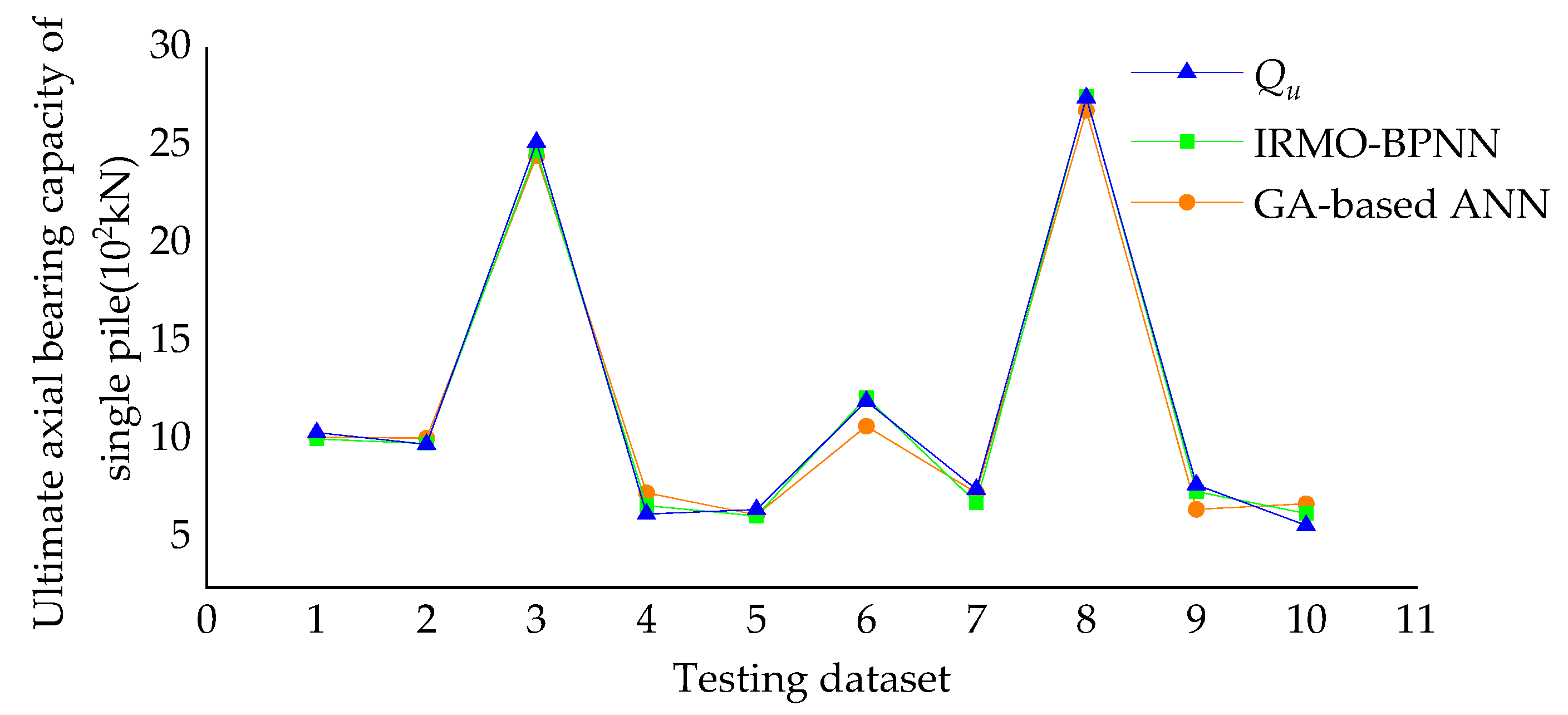
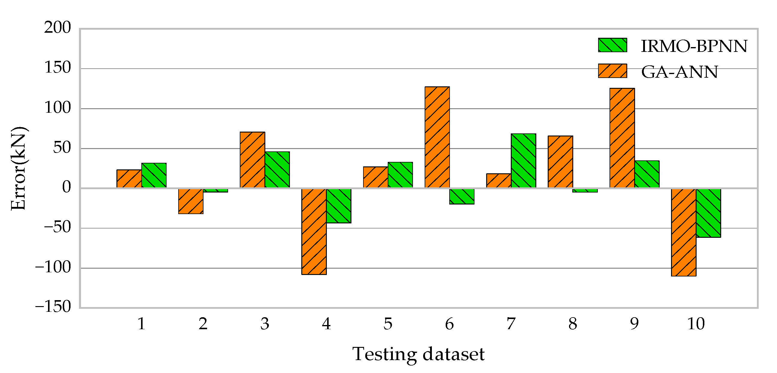
Both the GA-based ANN and IRMO-BPNN use global optimization algorithms to optimize the weights and thresholds of a traditional ANN or BPNN, but they use different global optimization algorithms. Global optimization algorithms continuously generate and update individuals within a specific search scope and eventually find the global optimal or approximately optimal solution through continuous iterations. The GA algorithm produces new individuals by mating them in pairs, whereas the IRMO algorithm produces them randomly from a central location. Figure 13 and Figure 14 display the prediction outputs and errors of the IRMO-BPNN model and GA-based ANN model trained on data set 1. Table 4 contains a list of the two models’ performances. As can be seen, the IRMO-BPNN model’s predicted values are closer to the experimental values, and the model’s performance parameters show its superior prediction. Differences in the way individuals are produced may explain this result.

5.2.2. Comparison with the RBFANN Model

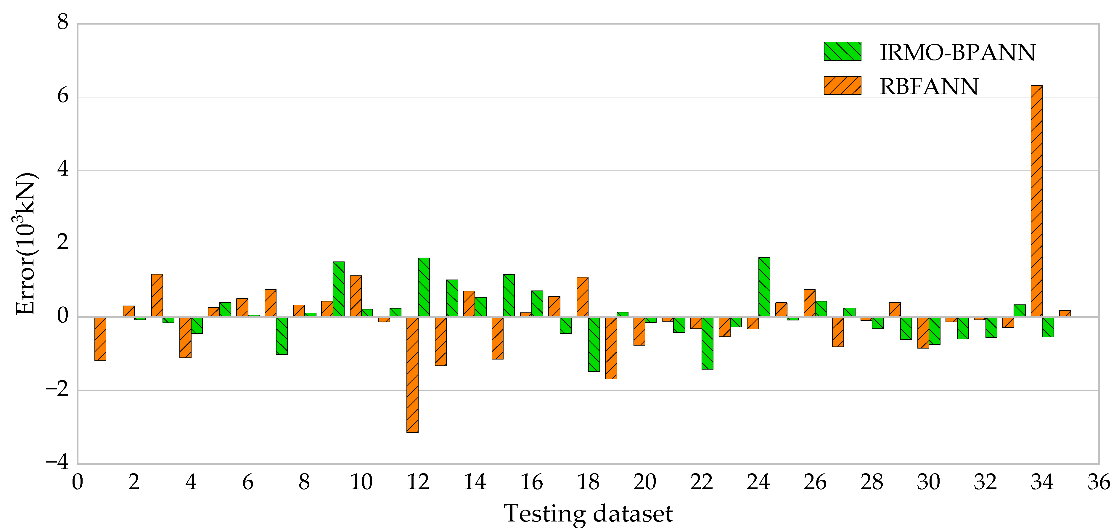
The RBFANN is an ANN that has a radial basis function of the activation function. It is a local approximation network that trains more quickly than an ANN and avoids falling into local optima. The prediction results and errors of the IRMO-BPANN model and RBFANN model trained on data set 2 are shown in Figure 15 and Figure 16. Table 5 shows the performance of the two models.
Overall, the predicted values of the two models are in good agreement with the experimental values. Nevertheless, the integrated IRMO-BPNN model resulted in fewer prediction errors than the single RBFANN model, especially for samples with large UABC (samples 12 and 34). Further evidence that a hybrid method outperforms the single ANN in terms of prediction performance comes from the fact that the R2 of the hybrid IRMO-BPNN model is 0.0155 larger than that of the single RBFANN model, and the MSE is almost 1/4 of that of the RBFANN model.

5.2.3. Comparison with the ANFIS-GMDH-PSO Model

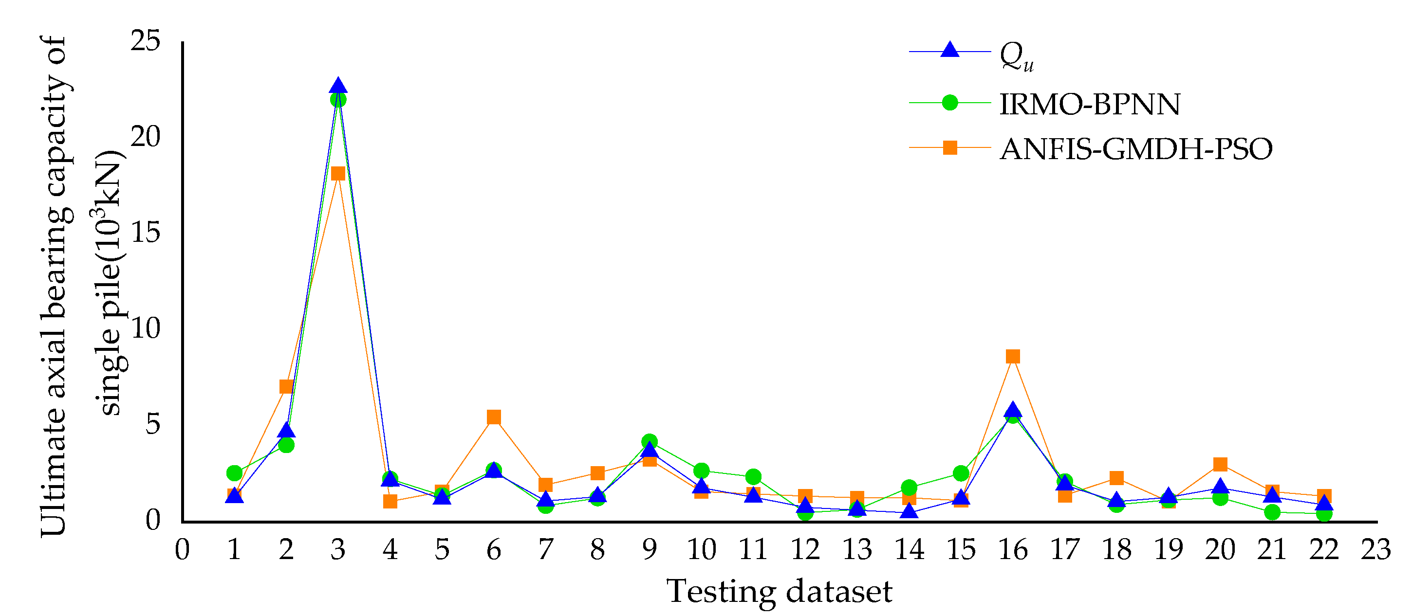
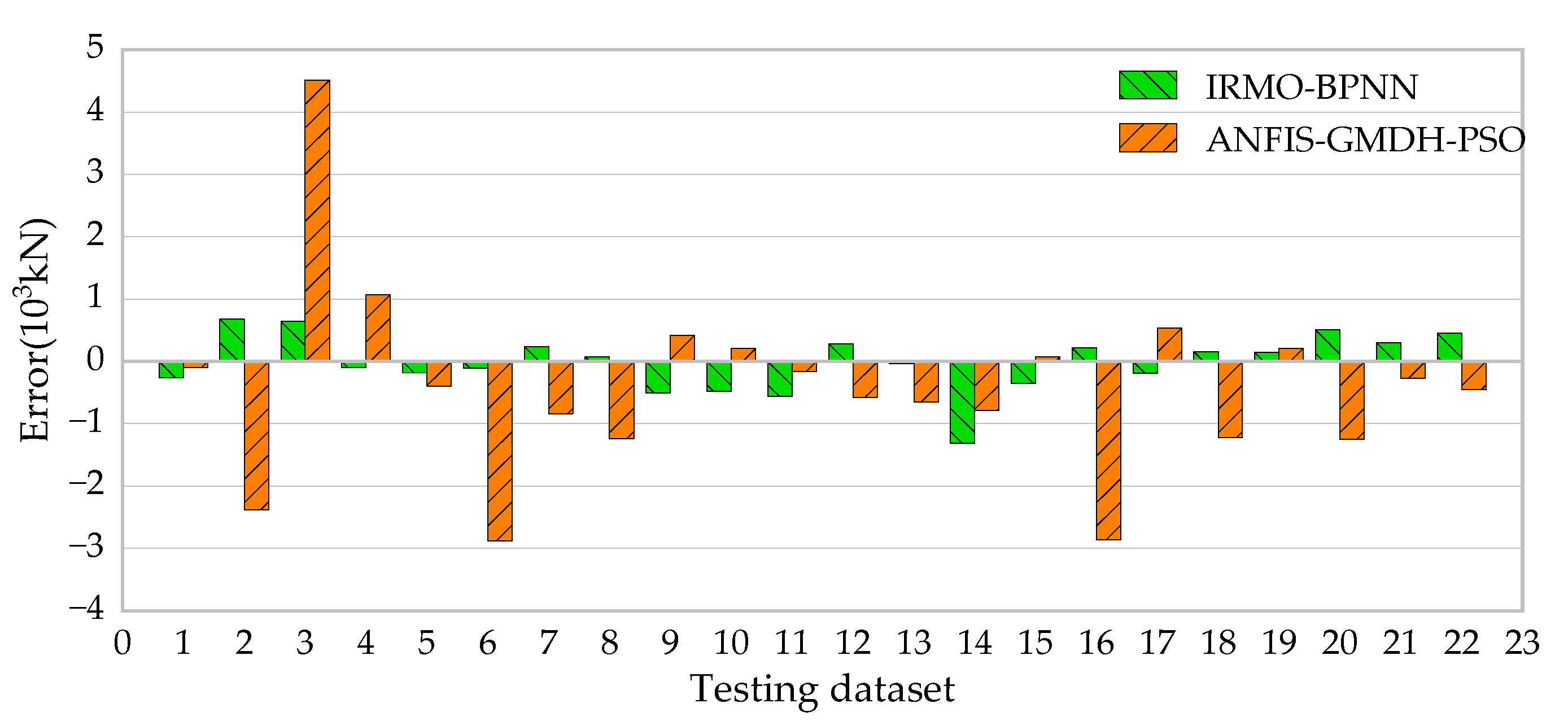
The ANFIS-GMDH-PSO model is an integration of the ANFIS, GMDH, and PSO algorithms, which firstly combines the adaptive-neuro-fuzzy inference system (ANFIS) with the group method of data handling (GMDH), and then optimizes the ANFIS-GMDH with the PSO algorithm. The prediction results and errors of the IRMO-BPNN model and ANFIS-GMDH-PSO model trained on data set 3 are shown in Figure 17 and Figure 18, and the performance of each is shown in Table 6. It can be noted that the predicted values of both models match the experimental values well, and some samples of the IRMO-BPNN model even have better-predicted values and performance parameters than those of the ANFIS-GMDH-PSO model. This suggests that for small-scale samples, the optimization performance of complex hybrid algorithms is not fully explored.
In summary, the predictive performance of the IRMO-BPNN model is superior to that of the GA-based ANN model, the RBFANN model, and the ANFIS-GMDH-PSO model in terms of prediction accuracy. When predicting individual samples with large UABC, the IRMO-BPNN model produces fewer errors, showing great superiority.

6. Conclusions

Based on a combination of the IRMO algorithm and a BPNN, a new network called IRMO-BPNN was proposed to solve the problems of BPNN prone to local optimal values, over-fitting, and unstable search results. After data processing and parameter optimization, the IRMO-BPNN model for predicting the UABC of a single pile was developed and compared with the GA-based ANN model, RBFANN model, and ANFIS-GMDH-PSO model. The following conclusions can be obtained:
(1)
Using a trial-and-error method, the optimal number of hidden nodes is 11 in this study. Hyper-parameters contribute to the IRMO-BPNN model being more accurate and with less prediction error as the population size and number of iterations grow. Additionally, increasing the model’s iterations is more effective in enhancing model performance.
(2)
The IRMO-BPNN model has good performance for predicting the UABC of a single pile. The model did not overfit in the iteration process, and the predicted value of the model is very close to the experimental value. The MAPE of the model is 4.86%, and the R2 of the training, verification, and testing sets are 0.98911, 0.98277, and 0.97030, respectively. During the iterative process, the MSE of the model decreases to stabilize gradually, and the results obtained from multiple runs are roughly the same, which indicates the great global optimization ability and search stability of the model.
(3)
The hybrid algorithm has been utilized to improve BPNN’s prediction performance. Compared to other hybrid algorithms, the IRMO-BPNN has a faster convergence rate, a higher prediction accuracy, and greater stability owing to its distinctive data structure.
The feasibility and superiority of IRMO-BPNN in predicting the UABC of a single pile are verified in this article. However, the IRMO-BPNN model established in this article still has geographical limitations and contains fewer data. Thus, the data set is being continuously enlarged and updated for further studies.

Author Contributions

Conceptualization, L.J. and Y.J.; methodology, L.J.; software, Y.J.; validation, L.J. and Y.J.; formal analysis, L.J.; investigation, Y.J.; resources, L.J.; data curation, Y.J.; writing—original draft preparation, Y.J.; writing—review and editing, L.J.; visualization, Y.J.; supervision, L.J.; project administration, L.J.; funding acquisition, L.J. All authors have read and agreed to the published version of the manuscript.

Funding

This research was funded by the Hunan Provincial Natural Science Foundation of China, grant number 2022JJ30724.

Data Availability Statement

Data available on request due to restrictions, e.g., privacy or ethics. The data presented in this study are available on request from the corresponding author. The data are not publicly available due to commercial use.

Acknowledgments

The authors are grateful for support from the Hunan Provincial Natural Science Foundation of China (2022JJ30724).

Conflicts of Interest

The authors declare no conflict of interest. The funders had no role in the design of the study; in the collection, analyses, or interpretation of data; in the writing of the manuscript; or in the decision to publish the results.

References

  1. Kordjazi, A.; Pooya Nejad, F.; Jaksa, M.B. Prediction of ultimate axial load-carrying capacity of piles using a support vector machine based on CPT data. Comput. Geotech. 2014, 55, 91–102. [Google Scholar] [CrossRef]
  2. Meyerhof, G.G. The ultimate bearing capacity of foundations. Géotechnique 1951, 2, 301–302. [Google Scholar] [CrossRef]
  3. Meyerhof, G.G. Bearing Capacity and Settlement of Pile Foundations. J. Geotech. Eng. Div. 1976, 102, 197–228. [Google Scholar] [CrossRef]
  4. Titi, H.H.; Abu-Farsakh, M.Y. Evaluation of Bearing Capacity of Piles from Cone Penetration Test Data; Louisiana Transportation Research Center: Baton Rouge, LA, USA, 1999. [Google Scholar]
  5. Seed, H.B.; Reese, L.C. The action of soft clay along friction piles. Trans. Am. Soc. Civ. Eng. 1957, 122, 731–754. [Google Scholar] [CrossRef]
  6. Davis, E.H.; Poulos, H.G. The Settlement Behaviour of Single Axially Loaded Incompressible Piles and Piers. Géotechnique 1968, 18, 351–371. [Google Scholar] [CrossRef]
  7. Randolph, M.F.; Carter, J.; Wroth, C. Driven piles in clay—The effects of installation and subsequent consolidation. Geotechnique 1979, 29, 361–393. [Google Scholar] [CrossRef]
  8. Ellison, R.D.; D’Appolonia, E.; Thiers, G.R. Load-Deformation Mechanism for Bored Piles. J. Soil Mech. Found. Div. 1971, 97, 661–678. [Google Scholar] [CrossRef]
  9. Hamed, M.; Emirler, B.; Canakci, H.; Yildiz, A. 3D Numerical Modeling of a Single Pipe Pile Under Axial Compression Embedded in Organic Soil. Geotech. Geol. Eng. 2020, 38, 4423–4434. [Google Scholar] [CrossRef]
  10. Chan, W.T.; Chow, Y.K.; Liu, L.F. Neural network: An alternative to pile driving formulas. Comput. Geotech. 1995, 17, 135–156. [Google Scholar] [CrossRef]
  11. Lee, I.M.; Lee, J.H. Prediction of Pile Bearing Capacity Using Artificial Neural Networks. Comput. Geotech. 1996, 18, 189–200. [Google Scholar] [CrossRef]
  12. Goh, A.T.C. Pile Driving Records Reanalyzed Using Neural Networks. J. Geotech. Eng. 1996, 122, 492–495. [Google Scholar] [CrossRef]
  13. Benali, A.; Nechnech, A. Prediction of the pile capacity in purely coherent soils using the approach of the artificial neural networks. In Proceedings of the Second International Conference on the Innovation, Valorization and Construction INVACO2, Rabat, Morocco, 23–25 November 2011. [Google Scholar]
  14. Benali, A.; Boukhatem, B.; Hussien, M.N.; Nechnech, A.; Karray, M. Prediction of axial capacity of piles driven in non-cohesive soils based on neural networks approach. J. Civ. Eng. Manag. 2015, 23, 393–408. [Google Scholar] [CrossRef]
  15. Rezaei, H.; Nazir, R.; Momeni, E.; Engineering, F.O.; University, L. Bearing capacity of thin-walled shallow foundations: An experimental and artificial intelligence-based study. J. Zhejiang Univ.-Sci. (Appl. Phys. Eng.) 2016, 17, 273–285. [Google Scholar] [CrossRef]
  16. Moayedi, H.; Jahed Armaghani, D. Optimizing an ANN model with ICA for estimating bearing capacity of driven pile in cohesionless soil. Eng. Comput. 2017, 34, 347–356. [Google Scholar] [CrossRef]
  17. Momeni, E.; Nazir, R.; Jahed Armaghani, D.; Maizir, H. Prediction of pile bearing capacity using a hybrid genetic algorithm-based ANN. Measurement 2014, 57, 122–131. [Google Scholar] [CrossRef]
  18. Armaghani, D.J.; Shoib, R.S.N.S.B.R.; Faizi, K.; Rashid, A.S.A. Developing a hybrid PSO–ANN model for estimating the ultimate bearing capacity of rock-socketed piles. Neural Comput. Appl. 2017, 28, 391–405. [Google Scholar] [CrossRef]
  19. Benali, A.; Hachama, M.; Bounif, A.; Nechnech, A.; Karray, M. A TLBO-optimized artificial neural network for modeling axial capacity of pile foundations. Eng. Comput. 2021, 37, 675–684. [Google Scholar] [CrossRef]
  20. Jin, L.X.; Feng, Q.X. Improved radial movement optimization to determine the critical failure surface for slope stability analysis. Environ. Earth Sci. 2018, 77, 564. [Google Scholar] [CrossRef]
  21. Jin, L.X.; Zhang, H.C.; Feng, Q.X. Ultimate bearing capacity of strip footing on sands under inclined loading based on improved radial movement optimization. Eng. Optimiz. 2021, 53, 277–299. [Google Scholar] [CrossRef]
  22. Rahmani, R.; Yusof, R. A new simple, fast and efficient algorithm for global optimization over continuous search-space problems: Radial Movement Optimization. Appl. Math. Comput. 2014, 248, 287–300. [Google Scholar] [CrossRef]
  23. Jin, L.X.; Feng, Y.W.; Zhang, H.C.; Feng, Q.X. The use of improved radial movement optimization to calculate the ultimate bearing capacity of a nonhomogeneous clay foundation adjacent to slopes. Comput. Geotech. 2020, 118, 103338. [Google Scholar] [CrossRef]
  24. Li, S.; Zhang, Q.; Zhang, Q.; Li, L. Field and theoretical study of the response of super-long bored pile subjected to compressive load. Mar. Georesources Geotechnol. 2016, 34, 71–78. [Google Scholar] [CrossRef]
  25. Gu, P.; Xiong, X.; Qian, W.; Zhao, J.; Lu, W. Grey relational analysis of influencing factors of bearing capacity for super-long bored piles. In Proceedings of the 2013 IEEE International Conference on Grey Systems and Intelligent Services (GSIS), Macau, China, 15–17 November 2013; pp. 57–61. [Google Scholar]
  26. Chen, Q.H.; Chen, G.Q.; Xie, R.B.; Zai, J.Z. Influence of the Penetration Depth into the Bearing Stratum on the Bearing Capacity of Single Pile. Chin. J. Geotech. Eng. 1981, 3, 16–27. [Google Scholar]
  27. JGJ 94-2008; Technical Code for Building Pile Foundations. China Building Industry Press: Beijing, China, 2008.
  28. Tabachnick, B.G.; Fidell, L.S. Using Multivariate Statistics, 6th ed.; Allyn and Bacon: Boston, MA, USA, 2013. [Google Scholar]
  29. Stone, M. Cross-validatory choice and assessment of statistical predictions. J. R. Stat. Soc. Ser. B (Methodol.) 1974, 36, 111–147. [Google Scholar] [CrossRef]
  30. Harandizadeh, H.; Toufigh, M.M.; Toufigh, V. Different neural networks and modal tree method for predicting ultimate bearing capacity of piles. Int. J. Optim. Civ. Eng. 2018, 8, 311–328. [Google Scholar]
  31. Harandizadeh, H.; Jahed Armaghani, D.; Khari, M. A new development of ANFIS–GMDH optimized by PSO to predict pile bearing capacity based on experimental datasets. Eng. Comput. 2021, 37, 685–700. [Google Scholar] [CrossRef]
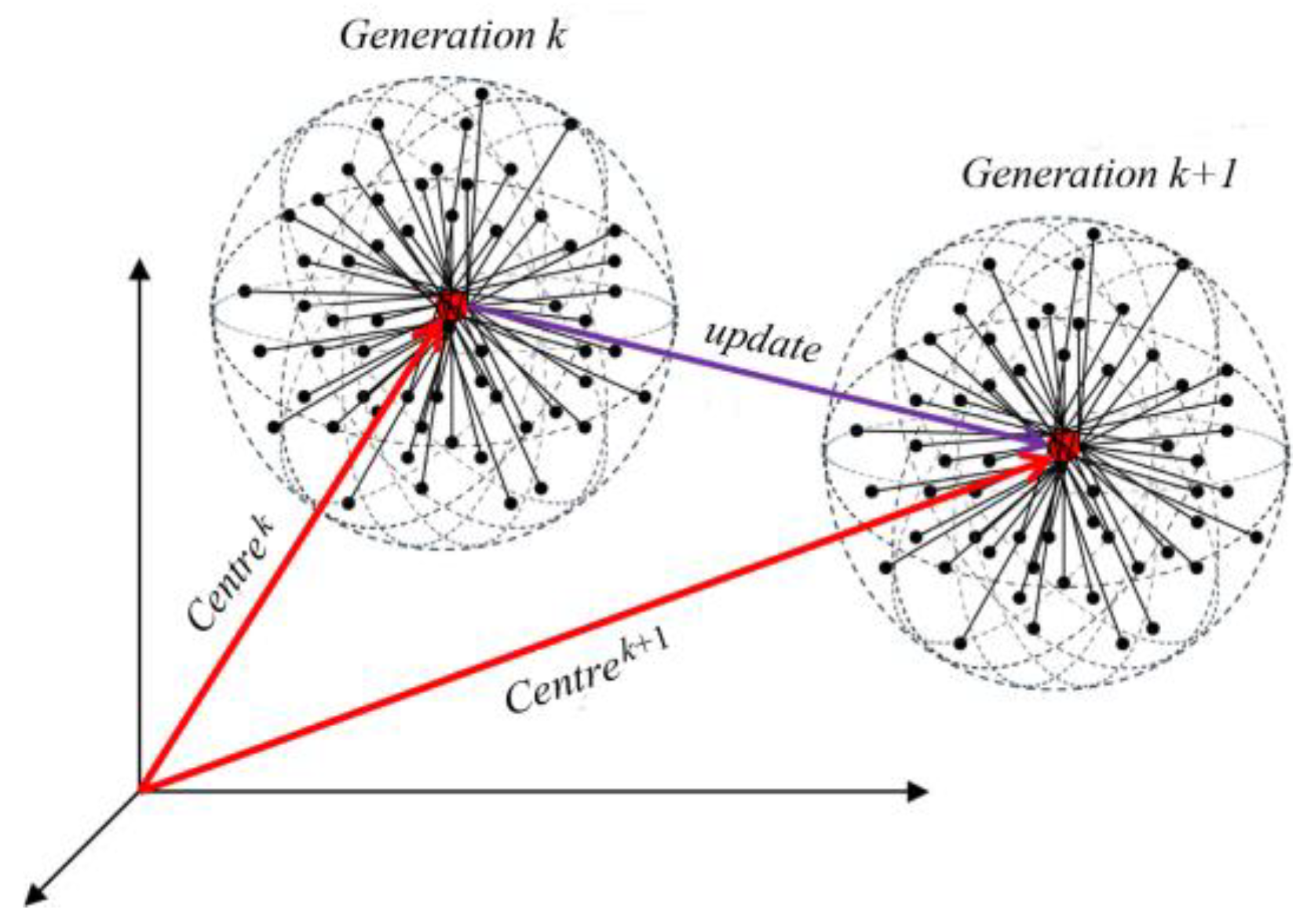
Figure 1. Diagram of the radial movement algorithm (RMO).
Buildings 13 01297 g001
Figure 2. The flowchart of the IRMO algorithm.
Buildings 13 01297 g002
Figure 3. Typical BP neural network (BPNN) architecture.
Buildings 13 01297 g003
Figure 4. The flow chart of IRMO-BPNN.
Buildings 13 01297 g004
Figure 5. Data sets used in the IRMO-BP neural network (IRMO-BPNN) model.
Buildings 13 01297 g005
Figure 6. Model performance of different hidden nodes.
Buildings 13 01297 g006
Figure 7. (a) The impact of the nop on model performance; (b) The impact of the g on model performance.
Buildings 13 01297 g007
Figure 8. (a) Iteration process of the BPNN model; (b) iteration process of the BPNN model optimized by the IRMO algorithm.
Buildings 13 01297 g008
Figure 9. Comparison between the experimental values and predicted values.
Buildings 13 01297 g009
Figure 10. Determination coefficient of the BPNN data sets.
Buildings 13 01297 g010
Figure 11. Determination coefficient of the IRMO-BPNN data sets.
Buildings 13 01297 g011
Figure 12. Change curve of the MSE during iteration.
Buildings 13 01297 g012
Figure 13. Predicted values of the GA-based ANN model and IRMO-BPNN model.
Buildings 13 01297 g013
Figure 14. Comparison of testing sample errors between the GA-based ANN model and the IRMO-BPNN model.
Buildings 13 01297 g014
Figure 15. Predicted values of the RBFANN model and IRMO-BPNN model.
Buildings 13 01297 g015
Figure 16. Comparison of testing sample errors between the RBFANN model and IRMO-BPNN Model
Buildings 13 01297 g016
Figure 17. Prediction values of the ANFIS-GMDH-PSO model and IRMO-BPNN model.
Buildings 13 01297 g017
Figure 18. Comparison of testing sample error between the ANFIS-GMDH-PSO model and the IRMO-BPNN model.
Buildings 13 01297 g018
Table 1. Statistics of the data sets.
Data SetStatisticsInputsOutput
L (m)D (m) c ¯ φ ¯ qpk (kPa)Qu (kN)
TrainMax25.61.055.3631.72360017,400
Min3.40.530.5420.388003100
Average11.40.743.1226.2520298996
StD4.30.26.502.969652990
ValidationMax26.41.055.2631.35360017,100
Min3.50.531.5220.458003300
Average11.90.742.5626.2420549095
StD5.10.26.672.839653189
TestingMax26.91.055.2531.50360017,300
Min3.90.531.7220.438003400
Average11.90.743.4326.4520479040
StD5.30.26.942.939673139
AllMax26.91.055.3631.72360017,400
Min3.40.530.5420388003100
Average11.60.743.0726.2920389025
StD4.70.26.632.939653046
Table 2. Performance parameters of models with different g and nop values.
nopgMAPEMSERMSER2VAF
202012.98%0.000470.02170.9768098.91
3012.63%0.000470.02170.9786299.14
4010.46%0.000460.02140.9791399.15
509.49%0.000450.02120.9798499.24
1007.91%0.000410.02020.9815199.48
302012.51%0.000470.02170.9784299.08
3010.36%0.000460.02140.9794199.21
408.77%0.000430.02070.9804899.27
507.78%0.000400.02000.9810799.31
1006.81%0.000390.01970.9816699.52
40209.89%0.000450.02120.9787599.15
308.64%0.000430.02070.9801299.24
407.04%0.000390.01970.9811199.38
506.30%0.000380.01950.9814599.46
1005.69%0.000370.01920.9819499.56
50208.44%0.000420.02050.9797499.23
306.81%0.000390.01970.9806099.28
406.21%0.000370.01920.9812399.46
505.12%0.000360.01900.9815999.50
1004.86%0.000360.01900.9834599.73
Table 3. Data sets used for model comparison.
Data SetCases
TotalTrainingTesting
Data set 1 [17]504010
Data set 2 [30]1006535
Data set 3 [31]725022
Table 4. Performance of the GA-based ANN model and IRMO-BPNN model.
ModelData SetR2MSERMSEVAFError MeanError StD
GA- based ANNTraining set0.96000.01150.1072- *- *- *
Testing set0.99000.00200.044798.882184
IRMO-BPNNTraining set0.99480.00040.020799.83−268
Testing set0.98960.00060.023699.72881
* no available data.
Table 5. Performance of the RBFANN model and IRMO-BPNN model.
ModelData SetR2MSERMSEVAFError MeanError StD
RBFANNTraining set0.9976208444457- *0460
Testing set0.97852045084143097.89−91451
IRMO-BPNNTraining set0.99927254626999.91−29270
Testing set0.994055319474499.3831754
* no available data.
Table 6. Performance of the ANFIS-GMDH-PSO model and IRMO-BPNN model.
ModelData SetR2MSERMSEVAFError MeanError StD
ANFIS-GMDH-PSOTraining set0.88360.00200.0480- *−0.00040.0480
Testing set0.92160.00500.069089.48−0.02100.0670
IRMO-BPNNTraining set0.98680.00030.016298.680.00620.0151
Testing set0.98010.00090.029897.96−0.00570.0299
* no available data.
Disclaimer/Publisher’s Note: The statements, opinions and data contained in all publications are solely those of the individual author(s) and contributor(s) and not of MDPI and/or the editor(s). MDPI and/or the editor(s) disclaim responsibility for any injury to people or property resulting from any ideas, methods, instructions or products referred to in the content.