Abstract
Developing methodologies to accurately characterise the energy conditions of existing building stock is a fundamental aspect of energy consumption reduction strategies. To that end, a case study using a thermal information modelling method for existing buildings (as-is T-BIM) is reported. This proposed new method is based on the automatic processing of 3D thermal clouds of interior zones of a building that generates a semantic proprietary model that contains time series of surface temperatures assigned to its surface elements. The proprietary as-is T-BIM automatically generates an as-is BEM model with gbXML standards for energy simulation. This is a multi-zone energy model of the building. In addition, the surface temperature data series of the as-is T-BIM model elements permit the calculation of their thermal transmittances, increasing the calibration options of the obtained as-is BEM model. To test the as-is TBIM method, a case study compares the as-is BEM model obtained by as-is T-BIM methods with the one obtained by standard methods for the same building. The results demonstrate differences in geometry, transmittance, and infiltration values, as well as insignificant differences in annual air conditioning energy consumption or the comfort parameters tested. This seems to indicate shorter modelling times and greater accuracy of the as-is T-BIM model.
1. Introduction
Buildings are a major contributor to climate change, accounting for one-third of global energy consumption and one-quarter of CO2 emissions [1]. Within the European Union, 40% of total energy consumption corresponds to the building sector. Approximately 35% of EU buildings are older than 50 years, and roughly 75% are energetically inefficient [2]. Energy efficiency regulations are imposing increasingly restrictive limitations intended to reduce such high levels of energy consumption. Very strict energy requirements are now imposed that guide the construction of nearly zero-energy buildings [3]. The justification of compliance with these standards is based on the use of building energy performance simulation (BEPS) procedures, which normally consist of the completion of a series of calculations that characterize the thermodynamic behaviour of the buildings at all hourly intervals over an annual period. At present, the generation of building energy modelling (BEM) is essential for energy simulation procedures to justify compliance with standards on building design, construction, and rehabilitation within the European Union [4,5].
In this scenario, building retrofitting is an important focus for the reduction of energy consumption. Consequently, developing methods to accurately characterise and represent the existing conditions of these buildings so as-is BEM is an important field of research. Building energy management is more effective with BEM integrated into building information modelling (BIM) methods [6]. However, it should be noted that the BIM to BEM process is a non-standard practise that produces building energy models that vary from user to user and from application to application [7]. Additionally, the energy modelling process is not fully incorporated into the digital process since the data acquisition and model implementation processes are tedious and require specialist operators [8]. It is therefore important to achieve greater automatization of BEM and better integration with the set of BIM management methods in building construction projects [8,9,10], taking into account that energy modelling is necessary for the initial phases of building projects [11,12,13]. In the field of energy modelling of existing buildings, a current topic of research and innovation is the incorporation of thermographic technologies that incorporate three-dimensional unstructured thermal point cloud data into processes [14,15,16,17]. Exploiting the dense thermal cloud information, i.e., geometry and temperature, is of great interest to the as-is BEM [18]. Thermal point clouds of as-is buildings have proved to be a relevant topic in as-is BIM research, especially in the last few years [17]. It can be stated that, to date, only simple thermal as-is BEM models of single constructive elements have been defined, and there is a long path to follow to automatically obtain a thermal as-is BEM model of a multi-story building [19]. In earlier research, we tested 3D thermal scanning platforms composed of a 3D laser scanner, an RGB camera, and a thermal camera that scans for 360° thermal data [20,21,22]. These works focused on the automation of the acquisition of 3D geometric and thermal clouds and the processing of this information. This technology has been successfully applied for monitoring the indoor temperatures of buildings, and detailed, remote, and precise analyses of the resulting 3D thermal visualization of surface temperature distributions and their variation over time can then be prepared [21]. The case study presented is based on obtaining a semantic as-is T-BIM proprietary model by processing a series of spatial and temporal thermal clouds of these spaces. The as-is T-BIM model has made it possible to automatically obtain a standard multi-zone gbXML file for energy simulation as well as an hourly series of surface temperatures for each of the classes of elements in each thermal zone.
The research interest in the use of building thermal clouds is based on the relevance of thermographic techniques for the qualitative and quantitative analysis of the thermal performance of buildings. In general, thermographic inspection requires adequate knowledge and control of the environmental parameters during the measurement tests due to the infrared configurations of most systems [23]. There are standardised procedures for that purpose [24], based on the qualitative analysis of the surface thermal maps shown in the thermographs, which, when properly analysed can indicate hidden or unexpected elements or certain pathologies to consider in as-is BEM. Infrared technology (IRT) is also used for quantitative purposes [25,26,27,28]. It is important to consider that the temperatures of indoor thermographic surface measurements present greater reliability than those measured outdoors. A difference is due to the variability of the air-convection effect, which influences indoor readings less than outdoor IRT readings [29]. In this way, the calculations of the Uvalue based on indoor IRT measurements are of greater reliability [28]. In our research, findings derived from the application of conventional thermography to building behaviour are considered both in the interpretation of the thermal point clouds and their processing for incorporation into the as-is BEM models.
Moreover, a specific issue with the as-is BEM addressed by our research is the need to calibrate these models with experimental data to reduce the uncertainty of the BEPS results. The parameters that define the energy efficiency of as-is buildings that are calculated through as-is BEM simulation models correspond to energy demand and consumption [4]. Likewise, as-is BEM has also been used to predict the thermal comfort of users through the calculation of the necessary environmental parameters, such as temperature, relative humidity, and air speed [30]. In any case, it should be noted that BEPS results will reflect a degree of uncertainty due to the difficulty of defining parametric models sufficiently adjusted to the reality of the building or the final conditions in service, according to the case. Normally, uncertainties are related to the material nature of the elements to be modelled and the service conditions envisaged for the building. On occasion, uncertainties can be due to the supply of weak meteorological information or difficulties with the estimation of air infiltration, surface thermal resistance, and the thermal performance of materials in a transitory regime [31,32,33]. The reduction of uncertainty is therefore an important field of research in relation to BEPS methods [34]. There are various calibration methods, among which the most frequently used are based on statistical comparisons between one or more parameters from the simulations and data from real measurements taken under the same environmental and service conditions as used in the simulation. The calibrations are achieved through the adjustment of these variables until the statistical values for comparison are within acceptable tolerance thresholds for each study [33]. Guidelines and protocols such as ASHRAE Guideline 14 (AG14) [35], the International Performance Measurement and Verification (IPMVP) [36], or theFederal Energy Management Program (FEMP) [37] provide recommendations on admissible tolerances and calibration criteria for models using statistical procedures applied to a comparative analysis of simulation results and sensor-monitoring data [33]. AG14 references are frequently used for the calculation of building energy demand and consumption in energy rehabilitation studies [38,39,40,41,42]. Some researchers have found that these acceptable ranges can be achieved even though there is a significant difference in the hourly distribution between the simulated and measured indoor temperature data. These authors base their calibrations on indoor temperature data with narrower tolerance ranges [40].
Another relevant aspect related to as-is BEM uncertainty is the determination of the thermal transmittance value (Uvalue) of the envelope elements of thermal zones. The Uvalue is defined as the quantity of heat that is transmitted through a certain material by a unit of area and time [43]. The nominal Uvalue of any constructive system may be calculated starting with values obtained from tables of physical and material properties and using calculations based on the principles of Fourier’s Law in stationary environmental conditions. Normally, the necessary physical parameters can be found in local [44] and international [45] standards, as is the case with the thermal resistance coefficient (R) and convection coefficients (hc). The Uvalue of a constructive system can also be measured by using heat flow measurements (HFM) [46], or through the simultaneous use of indoor and outdoor thermometers, in the same way, as indoor surface temperatures are monitored using surface sensors or by quantitative thermographic techniques [47,48,49]. When measuring the in situ thermal transmittance of some building elements and comparing the results with the theoretical values, a difference ranging from 14% to 43% has been found [50]. Therefore, the in-situ thermal property measurement of the elements is relevant for reducing performance gaps between the real buildings and the BEM as-is.
In this paper, the method that we have named the thermal building information models for existing buildings (as-is T-BIM) facilitates the modelling and calibration procedures of as-is BEM. The methodology is based on the use of data from three-dimensional thermographic scanning of indoor surfaces in the thermal zones of the building. This diagnostic system automatically generates as-is 3D-T thermographic point clouds of building zones, a proprietary semantic model (as-is T-BIM) with hourly surface temperature series associated with the elements of each thermal zone, and an as-is BEM gbXML standard schema for use with compatible energy simulation software. The research aims to integrate and test the acquisition of time series of thermal point clouds of the interior surfaces of buildings in both the automatic generation of multi-zone as-is BEM and the calibration of obtained thermal multi-zone BEM models, which are fundamentals in the simulation of existing building energy performance. To accomplish that, the as-is T-BIM method was tested with predictive thermal behaviour studies of a block of five thermal zones of a service-industry building. That same case study was also tested with a standard method (as-is STD) and simulated under the same predictive conditions. Finally, the results from the application of both methods, as-is T-BIM and as-is STD, to the same building were compared.
In the following section, the two methodological proposals of “as-is BEM” for simulations of existing buildings and “as-is STD” and “as-is T-BIM” are explained. In Section 2, the case study is also presented. Subsequently, in Section 3, the results of the predictive simulation of both models are presented and discussed. Finally, in Section 4, the conclusions of the investigation and expected future advances for the development of this research are provided.
2. Materials and Methods
In this section, the as-is T-BIM method and an existing building energy modelling standard that we refer to as as-is STD are explained. These methods are applied later in the case study. The STD method is a common approach based on the AG14 specifications [34] for existing buildings and tolerance values found in the literature regarding the calibration of models with indoor temperature data [40]. As shown in Figure 1, both methods, as-is STD and as-is T-BIM, provide semantic BEM models in standard schema (gbXML), which are imported to a standard energy simulation software package for performing predictive studies.
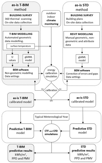
Figure 1.
Diagram of research procedures and results.
The diagram in Figure 1 depicts the phases of data collection, modelling, simulation, and results. There are different procedures during the data collection and modelling phases, as well as for inputs in the calibration phase procedures for Conduction Transfer Functions (CTF) simulations and contour parametrization in the Computational Fluid Dynamics (CFD) simulations. The differences arise mainly from the 360° data collection technique and the degree of modelling automatization and its procedures. In particular, the as-is STD method is based on manual data collection modelling procedures. In contrast, the as-is T-BIM method generates hourly series of point clouds and uses automatic procedures for modelling the geometry of elements and assigning temporal series to them with average surface temperature values. This information on surface temperatures facilitates the calibration of the models that are used in the heat transfer models with conduction transfer functions (CTF).
2.1. Building Survey
The generation of as-is STD models begins with the collection of data on the current state of the thermal zones of a building. Data collection consists of the identification of those thermal zones and the measurement of the constructive elements that constitute them. It also includes the compilation of data related to the available modes of usage and the service systems that are available. In the best of situations, the geometric and constructive information of the building can be found in existing documentation, although it will always have to be verified in situ. It will also be important to have monitoring systems in the indoor thermal zones of the buildings, as well as outdoor climate data for the same time period as the indoor monitoring.
The as-is T-BIM method provides an automated measurement system based on the use of a laser scanner and 360° thermographic camera, which provides the geometry of the zones and surface thermal information in the form of point clouds for each zone of the building. The surface thermal information of each thermal zone and its contours is complemented with information from the monitoring systems of atmospheric temperature (Tatm) and relative humidity (RHatm). The sensor system used for as-is T-BIM data collection is composed of a medium scan range 3D scanner, a high definition (HD) colour camera, and a thermographic camera. This system is successively applied to the different zones of a building. The XYZ coordinates of each zone generated by the sensor, a set of RGB images, and another set of IRT images are all stored. The processing of all this information generates a set of point clouds for each zone, or, in other words, a set of 3D coordinates referring to a shared system where each point has a red–green–blue (RGB) colour and an apparent associated temperature. In our case, the measurement frequency is 1 h intervals, completing one scan and five 360° thermographic snapshots per zone. The five snapshots are then synthesised into a unique average thermal point cloud with better precision. The apparent surface temperature values are in the order of 2 points/cm2 (Figure 2).
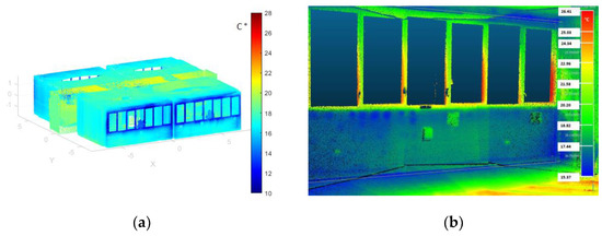
Figure 2.
As-is T-BIM thermal point-cloud: (a) perspective of the block of five thermal zones; (b) indoor view of a thermal zone.
The apparent surface temperatures (Tapp.surf) of each point that the thermal system initially generates are corrected with the emissivity (ε) parameters of each material and the reflected temperature (Tref) recorded on each wall. A sealant tape and wrinkled aluminium foil are placed over the basic elements of the envelope, a blackbody and a Lambert stove, respectively (Figure 3). The apparent temperatures of these objectives will serve for the automatic calculation of indoor surface temperature and the real temperature of each point.
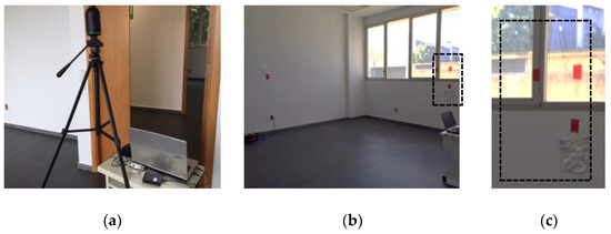
Figure 3.
(a) 3D geometric and thermal scanner; (b) Perspective of one of the rooms of the case study; (c) Detail of the objectives for reading the parameters Tref and ε.
The corrected values of the point-cloud temperatures will be used for the calculation of the average surface temperatures (Tavg.surf). These average temperatures will be used to figure out the U value of the building envelope and its parts and to calibrate the T-BIM model for the CTF simulation of the rooms. Likewise, the average temperature calculated for each element of the thermal zones may be used as contour temperatures in the case of CFD simulations conducted for the study of the thermal comfort of the rooms.
2.2. Modelling
as-is BEM generates 3D geometric models of indoor building zones, formed of simplified surface elements, under the requirements of the energy simulation software. The data and properties required for the calculation of energetic balances are assigned to the geometric elements of the BEM models. In the case of an as-is STD method, the use of standard graphic environments (DesignBuilder) compatible with gbXML for generating the simulation models with EnergyPlus will be used as a calculation engine for CTF-type simulations. Standard BIM software will be used (Autodesk Revit) for modelling and the assignment of material and zone-related properties (air infiltration, internal loads, etc.) and to transfer them through the standard gbXML schema to the simulation software. This alternative may present problems of interoperationality.
The principal feature of the as-is T-BIM methodology is the storage of a temporal series of geometric point clouds (3D-T) with dense information on surface temperature, which will be synchronised with temperatures and atmospheric relative humidities of both the indoor and outdoor thermal zones. The 3D-T point clouds are compatible with mainstream visualisation or point-cloud processing software, such as CloudCompare in this case. Visual imaging of thermal zones and their elements, the establishment of colour scales for the temperatures, consulting specific temperatures and regional point-cloud averages, and the labelling of regions can be performed with these programs, among other options, and will be used to form a qualitative inspection of the 3D-T model. In addition, to obtain an as-is T-BIM model, 3D-T point-cloud segmentation, recognition, and classification of regions will be processed. Through data processing, a 3D semantic model will be generated where the geometries of the fundamental object classes of the building (walls, floors, ceilings, spaces, doors, and windows) are defined as they exist when capturing the images with the thermal scanner (see [22] for more information). These models are supplied with the temporal series of the average surface temperature values (Tavg,surf) of each element. The calculation of Tavg,surf is carried out after measuring each of the ortho-thermal images corresponding to each fundamental object.
Additionally, when adequate climatic conditions have been achieved at the time of collecting the data, the as-is T-BIM model can be complemented with the Uvalue corresponding to the opaque elements of the envelope. The method that Blanca Tejedor [42] proposed was used to calculate the transmittance values using Equation (1).
where U [W/m2 K] is the thermal transmittance Uvalue; Tref is the reflected temperature; Tsurf,ind is the indoor surface temperature; Tind is the indoor atmospheric temperature; Tout is the outdoor atmospheric temperature; hc is the convection coefficient; ε corresponds to the emissivity of the material; and σ is the Stefan-Boltzmann constant.
Finally, the data gathered with the as-is T-BIM method are transferred to the energy simulation software through conversion to BEM standard schema such as IDF and gbXML (Figure 4). The models that are generated contain geometric and semantic elements that meet BEM standards for average surface temperatures and thermal transmittance values. Adjacent properties are added to these contour and envelope elements, which are necessary to constitute the models of the building zones as a set of different thermal zones.
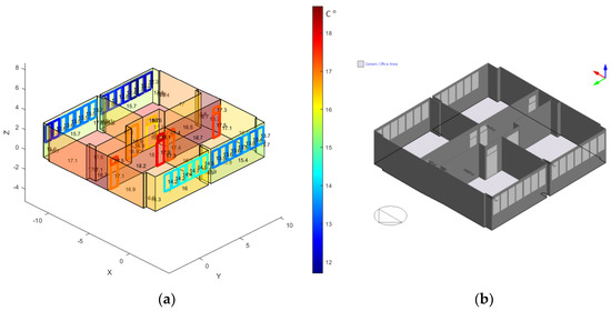
Figure 4.
(a) T-BIM model, with surface temperatures in its viewer. (b) GBXML model of adiabatic adjacencies and envelope transmittance calculated with the DesignBuilder viewer.
2.3. Simulation and Calibration
The simulation tests of building energy demand and consumption were performed with different commercial and CTF-type open-source numerical calculation software. Among them, Trnsys and EnergyPlus stand out because of their popularity when conducting tests for scientific, academic, and professional purposes. Different IDF and gbXML schemas enhance the inter-operationality of the models obtained with the as-is STD and as-is T-BIM methods and the simulation software. Therefore, the simulation phase is similar for both methods, given that the input is already the standard simulation model, whether obtained with either as-is STD or T-BIM. Differences are established in the calibration procedure, given that as-is T-BIM displays more thermal information, the Tavg.surf, and the Uvalues of envelope elements.
In general, a comparative analysis will be necessary between the simulation results and measurements completed in the monitoring phase for the calibration of any as-is BEM. As mentioned in Section 1, this type of study consists of the completion of statistical analyses that shed light on the deviations between the simulated results and the measurements. The indoor atmospheric temperature values of the thermal zones are frequently used for these calibrations. Others can also be used, such as energy consumption, as recommended in AG14-BCSA [35], IPMVP [36], or FEMP [37] when providing the statistical parameters and the limit deviations for the simulation results to be used in the calibration procedures. In our research, where the calibrations are based on indoor temperature data, we use narrower tolerance ranges based on the literature [40] (Table 1).

Table 1.
Statistical criteria for calibration were applied in the investigation.
In calibration procedures, BEM parameter adjustments can be made to one or several parameters simultaneously. Normally, the parameters subject to these adjustments will be those that are difficult to establish, such as the albedo coefficient, soil temperatures, infiltration rates, transmittance coefficients of the envelope elements, and internal loads, among others.
The thermographic point clouds that are generated and synchronised with the indoor and outdoor atmospheric information open up new possibilities for the analysis of the most common data in the calibration procedures. It means that qualitative and quantitative thermal analysis of both contour elements and all the zones together can be performed in as-is T-BIM through the temporal series of surface temperatures. In particular, the temporal series of surface temperatures can be used in the calibration tasks of the models through the adjustment of transmittances of envelope elements, as explained in Section 3.2.
On the other hand, CFD-type simulations typical of studies of thermal comfort inside buildings can also be carried out. The spatial distribution of the comfort parameters may be calculated with this type of simulation, provided that the contour parameters of the area under simulation are known. Normally, the as-is STD methods will establish the contour parameters of the simulation domain, coupled with the simulation results of the calibrated as-is STD model. Those contour parameters are the Tatm of the simulation domain, the Tavg.surf of the simulation domain limits (i.e., the walls and ceilings), intake and outtake vents, infiltration heat loss, and the openings within the thermal zone that is to be simulated. as-is T-BIM, on the contrary, facilitates the generation of geometric models and the automatic establishment of measured surface temperature contour values. This information can be directly employed, without previous CTF simulation, when the information on the other contour parameters is available.
2.4. Analysing Results
Predictive tests are designed for the calibrated as-is BEM of the thermal zones of the buildings (calibrated as-is BEM is the modelling of energy that, when simulated under certain conditions, will produce the results within the admissible tolerances). Generally, those tests are intended to predict the energy behaviour of a calibrated as-is BEM whenever materials, utilization, or climatic conditions are modified to its calibrated conditions, normally for energy savings, and improved user comfort. The predictions will correspond to the difference between the thermal balances of the CTF simulation of the as-is zones of the model and those of the modified zones. These results are expressed in terms of energy demand (kWh/m2·year) and energy consumption (kWh/m2·year).
Tests were also conducted to predict degrees of user comfort. Those predictive studies can be based on the analysis of indoor atmospheric parameters—temperature (°C), relative humidity (%), air speed (m/s), rooms, and thermal zones—and on the application of methodologies to calculate comfort-related references. Among the various mathematical models used for the study of comfort, the Fanger mathematical model is often employed because of its ease of use and suitable graphic presentation. This method has been incorporated in ISO 7730 [30]. It must be accepted that if the results are not higher than the reference values in each evaluation, then the conditions for the user will be within the comfort range. The reference parameters are known as the predicted mean vote (PMV) and the predicted percentage dissatisfied (PPD). The range of results is between the values −2 < PMV < 2, and 5 < PPD < 100%. The values of admissible comfort are situated between −0.5 and +0.5 for the PMV and 5% and 10% for the PPD, with the end of each interval being the maximum admissible range.
To some extent, using calibrated as-is T-BIM as a foundation facilitates the completion of predictive BEM studies. The advantage that this method offers is based on the automatization of data collection processes for buildings and the automatization of the generation of input semantic models for energy simulations with greater geometric precision. Additionally, calibrated as-is T-BIM offers the possibility of conducting temporal surface temperature evolution analyses of thermal zones and, therefore, better knowledge of the thermal performance of the building. Calibration possibilities are of great importance, and they are presented based on a dense information series of the surfaces of the thermal zones. In general, it can be concluded that the increased precision of the base models, both in their geometry and in the values of their transmittance, reduces prediction uncertainties.
In Section 2.5, the application of both as-is BEM methods for obtaining two energy simulation models corresponding to the same building case study is described: a model generated with as-is STD methods (according to AG14 standards) and a second model generated according to the as-is T-BIM method. Both models will be used for the thermal characterization, heating and cooling (air-conditioning), and comfort demands of five zones of a building in a continental climate through simulations. With previously calibrated models, as-is STD and as-is T-BIM will be applied to various predictive studies: some based on CTF-type simulations, for predicting the air-conditioning and thermal comfort energy demands in stationary regimes for each zone; and others based on CFD simulations for calculating the spatial distribution of atmospheric comfort parameters in a thermal zone, in a stationary regime.
2.5. Case Study
This study aims to determine the scope of the T-BIM method. For this purpose, it is planned to compare the simulation results of the energy models generated with the as-is STD and as-is T-BIM methods. To accomplish this, two models of the same block of a building that differed in modelling and calibration methods were generated, as described in detail in Section 2.5.2 and Section 2.5.3. The five rooms that compose the block of the building were scanned with a 3D-T scanner to obtain the geometry of the as-is T-BIM model. The atmospheric temperature of Room W1 was monitored for 48 h, between the 17 and the 19 of November 2021. The 3D thermal scanner captured images of the room for 6 h, between 8:00 h and 14:00 h on 19 November, to characterise the indoor thermal evolution of the contour surfaces of the room up until the time it received direct sunlight. Having obtained them, the two models were first calibrated and later simulated using the meteorological climate data (TMY 2007–2021) corresponding to the locality of the building. The results were eventually analysed in a comparative study, forming the basis of the study’s conclusions.
2.5.1. Description of the Building
The building referred to as Espacio IDEAS-UCLM Emprende, which is located on the campus of the University of Castilla La Mancha, was constructed in 2016 with European Regional Development funds. The building project and its construction standards corresponded to the Código Técnico de Edificación (CTE)—Spanish Technical Building Code—in force that year [51]. Recommendations for HVAC may be found in the Reglamento de Instalaciones Térmicas de Edificios (RITE)—Building Thermal Installations Regulation—in force that year [51,52]. The building is within a Bsk climate zone according to the Köppen-Geiger climate classification [53].
The zones of the building that were analysed consisted of four office rooms distributed along a corridor, situated on the ground floor of the building and separated from the ground by a ventilated air chamber. The layout and dimensions of the five zones are shown in Figure 5. Two offices face an interior patio towards the east (Rooms E1 and E2), and another two face the grounds towards the west (Rooms W1 and W2), all interconnected along the interior corridor.
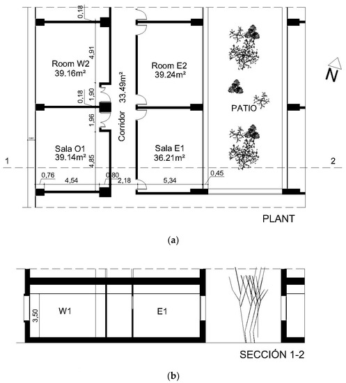
Figure 5.
General plans of the block of five thermal zones under study: (a) layout of the ground floor; and (b) sectional view.
According to the data on the execution project of the building, the office zones have a height of 3.5 m and similar floor areas, between 36 and 40 m2, approximately. The interior volume of each of these rooms is therefore between 126 m3 and 140 m3. The set of zones, including the corridor that connects them, represents a useful total surface area of 236 m2 and a volume of approximately 826 m3. The constructive and thermal characteristics that constitute these spaces correspond to the standards for the place and date of construction of the building. The main characteristics of the envelope appear in Table 2.
Table 2.
Thermal and constructive characteristics of the envelope elements and zonal separation.
The installations within these spaces consisted of fluorescent lighting tubes on the ceilings, electric power plugs on vertical walls, and mechanical ventilation and air-conditioning installations on the ceiling, in addition to emergency (lighting and fire detection) systems. The technical data of these installations can be consulted in Table 3.
Table 3.
Services are available in the rooms under study.
Each room is intended to house four office workstations. The dimensioning of the ventilation and air-conditioning installations corresponds to an occupation ratio of 0.1 per/m2. Ventilation grilles are therefore installed with intake air vents and diffusers for indoor heating and air conditioning. In each room, there is a small 10 × 20 cm intake air vent in the ceiling for fresh air from outdoors, with a heat recovery temperature control system rated at an efficiency value of 0.7. A variable refrigerant flow (VRF) system provides air conditioning for each room. Its indoor unit, installed over the suspended ceiling, provides air conditioning flows of 9 m3/min that are circulated through three circular air diffusers aligned in the central zone of the ceiling of each room and an extractor grille of 50 × 50 cm, also in the ceiling, in an area close to the windows of each room. The air conditioning settings are 21 °C in the winter and 24 °C in the summer. The corridor is not directly regulated by the air conditioning system and only has one grille in the ceiling of the indoor air extraction system that extracts stale air flows by filtration through the openings of each office. In non-holiday periods, the building is used twenty-four hours a day, seven days a week.
The VRF air-conditioning system of the building is zoned by rooms and can be independently turned off in each room. It was decided to deactivate the air-conditioning system when capturing the 3D-thermal scanning imaging to prevent interference due to the flow of heating/air-conditioning on the indoor surface temperatures and to understand the behaviour of the constructive systems of the envelope. Nevertheless, it could not be performed in that way in the area of the corridor due to the design conditions of the rest of the air-conditioning system. Likewise, neither could the mechanical ventilation system be turned off in any of the rooms. The parameters that established these conditions were reflected in the models used for the calibration and the design of the base models for the predictive models that were subsequently employed in both methods.
It is important to point out that, given that the object of study is a part of the ground floor and not of the whole building, the elements adjacent to the parts of the building that were not modelled were considered adiabatic. In concrete, the elements adjacent to the parts of the building that were not modelled (ceilings, southern walls in rooms E1, W1, and Corridor, as well as northern walls of rooms E2, W2, and Corridor) were considered adiabatic for both models. While heat transfer will apply to the adjacent elements that separate each of the five zones and the outdoors. In particular, the temperature of the ground at 20 cm beneath the ventilated under-floor air chamber was obtained with Equation (2)
where Tground is the temperature of the ground and Tatm is the outdoor atmospheric temperature. Equation (2) correlates the temperature of the ground with the average atmospheric temperature for each month of the year [54].
In our case, the average monthly environmental temperatures have been calculated from climate charts provided by the Agencia Estatal de Metereología (AEMET)—State Meteorological Agency—for Ciudad Real for November 2021 and the Typical Meteorological Year (TMY) 2007–21, respectively, employed for simulations of calibration and prediction of thermal behavior of the two models: as-i STD and as-is T-BIM.
2.5.2. Modelling as-is STD
The generation of the first simulation model, obtained with the as-is STD method, used project data validated in situ (Figure 4, Table 2 and Table 3), and the exterior climate provided by AEMET for Ciudad Real in 2021. The data for the operation of the building were provided by the building maintenance team and corresponded to the use of the building over the same period. The monitoring of indoor temperatures used for the calibration of the model was obtained after the installation of HEAT, a low-cost indoor monitoring system [55], based on SHT35 sensors [56], which recorded temperature and humidity values every 15 min. These data were converted into hourly temperature and relative humidity series for November 2021, which were used for as-is STD model calibration. The results are presented in Section 3.2.
The as-is STD energy model was generated for all five rooms by implementing the data with the modelling tools that provided the interface, DesignBuilder V6, for energy simulation with the EnergyPlus calculation engine. The STD model is shown in Figure 6a.
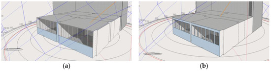
Figure 6.
gbXML model geometries in the DesignBuilder V.6 display interface. (a) as-is STD model; and (b) as-is T-BIM model.
2.5.3. Modelling as-is T-BIM
During the data collection, the areas being studied were empty, so there were no shadows on the walls that could affect the data. The air conditioning system was, in addition, turned off during the 3D thermographic scanning hours, while the ventilation continued to function according to the programmed settings for the rooms (Table 3). The temperature of each point in the point cloud of each captured image corresponded to the value of the real temperature that had been calculated. Thus, the temperature maps obtained for each wall at each hour of the day consisted of dense surface temperature information that can be used both for qualitative and quantitative analyses (Figure 7).
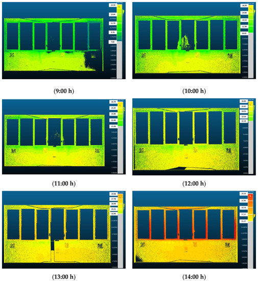
Figure 7.
Series of orthoimages of the western wall, Room W, 19 November 2021.
The processing of the point clouds automatically generated the geometry of the rooms in gbXML, which is compatible with various simulation software [57]. The choice of room and W1 for capturing the series of 3D thermographic images was due to its westerly orientation, which received no direct solar radiation between 7 p.m. and 13 a.m., on the date when the images were scanned. This allowed us to calculate the heat transmittance of the wall (Uvalue), the exterior aluminium window frames, and the floor using Equation (1) in Section 2.2.
Additionally, the dense thermal maps of the walls may be analysed qualitatively with the thermal model to test the lack of heterogeneity in the distribution of their temperatures and the detection of thermal points that are not present in the nominal model generated with the project data. In this way, we were able to test the temperature differences of the zones with thermal breaks within the substructures of lightweight partitions, insulation heat loss through masonry filling between the exterior carpentry of the window frames (lintels and jambs), and thermal infiltration loss through those structures (see Figure 8).
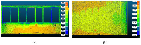
Figure 8.
Thermographic ortho-images obtained from the 3D thermal point cloud with real calculated temperatures: (a) indoor surface of the west wall of zone W, 10:00 h 19 November 2021; (b) indoor surface of the south wall of zone W, 10:00 h 19 November 2021. The colour palette changes with the temperature in steps of 0.4 °C to facilitate the visualisation of thermal surface differences.
3. Results and Discussion
Results of the geometry and the thermal behaviour of the as-is STD and the as-is T-BIM models are presented in this section. Specifically, we analyse the calibration results, the CTF predictive simulations, the energy behaviour of the building, and the comfort parameters. In addition, CFD simulation results in a stationary regime are also discussed.
3.1. Geometry of the Models
The geometric differences between the models obtained with the procedures corresponding to the as-is STD and the as-is T-BIM models were analysed. In the first case, the model was generated with the DesignBuilder modelling interface and the geometric data of the building project. In the second, the point clouds were automatically captured with the 360° thermographic scanner. Table 4 contains the surface values of the fundamental elements of the five zones for both models.
Table 4.
Geometric values of the elements in the as-is STD and as-is T-BIM models, totals and for each one of the zones. (1) percentage surface concordance of zones between the models.
Once verified in situ, the geometric magnitudes generated through the as-is T-BIM could be confirmed as being precisely adjusted to the reality of the building. The concordances between the surface values of the elements that comprised each of the models were 97% except in the case of the façade wall and the glazing, in which the metric differences were greater. The analysis of the semantic structuring of the elements demonstrated that it was different between models. The three elements of the exterior vertical enclosure were clearly distinguishable in the as-is STD model: the surface of the wall, the window frames, and the glazing of the building.
However, the surfaces of the window panes and the wall were all that were distinguishable in the as-is T-BIM model, and the carpentry surfaces were assimilated in the imaging of the surface of the wall in such a way that 78% of the image corresponded to the surface of the wall and 22% to the window frames installed in it. This point must be taken into account to objectify the existing differences between both models and in the comparative analyses of the simulation results of both the as-is STD and the as-is T-BIM models. In this way, it was confirmed that the differences between walls and glazing in the as-is T-BIM images approximated 95% of the surface images of the as-is STD model and that a dispersion of similar surfaces for all the elements was maintained between both models.
3.2. Model Calibration
In the model calibration process, simulation and monitoring results have been matched. Given the constructive and functional similarity of the four rooms of the building, the calibrations were carried out with the simulation and monitoring data of a single zone of the model, the south-western room (room W1). To accomplish this, hourly data of the atmospheric temperature of the room were collected between 18 and 19 November 2021, for a total of 48 h. A data series was also collected from the 360° thermal scans every hour, between 8 h and 14 h, on November 19. The six 3D thermographic models that were generated recorded the apparent, reflected, and blackbody temperatures of each material for all elements within the contours of the thermal zone. The average surface temperatures were obtained from the aforementioned series of values, in accordance with procedures presented in Section 2.2.
For the calibration of the as-is STD model, the indoor atmospheric temperature data obtained when monitoring room W1 were applied. Successive simulations and parametrical adjustments of infiltration were then performed, until acceptable tolerance thresholds were reached, according to the range of admissible tolerances for this study, see Table 1.
For the calibration of the as-is T-BIM, the infiltration heat loss values of the model were adjusted similarly, although the thermal transmittance values of the envelope had previously been calculated and adjusted with the data series of surface temperature measurements of the envelope elements within the thermal zone. The choice of room W1 for the completion of these tests was due to the absence of direct solar radiation on the wall of the façade during the morning hours. During the as-is T-BIM thermal scanning test, conducted on 19 May 2021, the absence of direct solar radiation on the façade was confirmed between 8:00 h, the test start-up time, and 13:10 h, the time at which the first rays of sunlight fell on the outdoor surface of the wall. The average thermal jump between the outdoor and indoor environments during this period was 8.4 °C. With these conditions, the U values of the outdoor façade elements were calculated, employing Equation (1), in Section 2.2. The input values were the average surface temperatures, the emissivity values, and the reflected temperatures calculated with thermographic temperature measurements, and the results are presented in Table 5. In this way, a global transmittance for this enclosure of 0.925 w/k m2 was obtained, as against the calculated nominal value of 0.908 w/k m2.
Table 5.
Input values and results for the calculation of exterior enclosure Uvalue of Room W1.
Subsequently, a Uvalue was obtained for the floor (Ufloor). The outdoor temperature of this element was not monitored. In the models that were used, a monthly value was applied. The thermal variation obtained with this procedure was not very high with regard to the indoor temperatures for the calculation of the transmittance of the floor. As an alternative, the Uvalue was adjusted until the surface simulation temperature (Tsurf.floor) reached the value of the data that were monitored, yielding a Ufloor transmittance value of 0.896 w/k m2. Finally, having adjusted the surface temperatures, the infiltration value was then adjusted using the atmospheric temperature values as a reference. In this way, it could be confirmed that the transmittance values obtained for the outdoor wall and the floor, together with the atmospheric temperature, provided simulated temperature values that were very close to the monitored values (Figure 9).
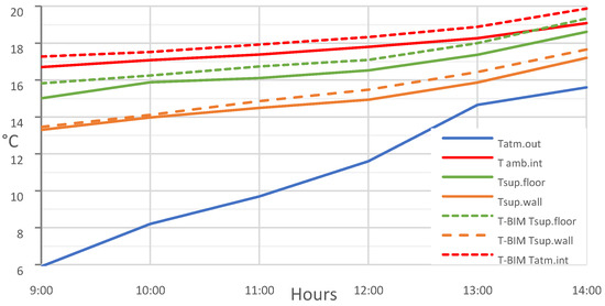
Figure 9.
Average simulation and monitored surface temperatures of the wall and the floor, of Room W1, 19 November 2021.
The comparison yielded wall and floor transmittance values with differences of −0.017 w/k.m2 and 0.436 w/k.m2, respectively, and infiltrations of 0.3 ren·h−1 in calibration tests. Therefore, using the STD method as a reference, important differences are determined in the transmittance of envelope elements and the infiltration level of the model in the calibration process of the as-is T-BIM.
As recommended in [40], for indoor temperature as-is building model calibration, we have calculated statistical parameters as limit reference deviations for the simulation results obtained in the calibration procedures. The calibration procedures that were employed for each model (as-is STD and as-is T-BIM) yielded admissible atmospheric temperatures according to the statistical tolerance limits established for this study (Figure 10) (Table 6).
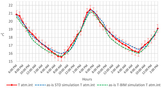
Figure 10.
Average simulation and monitored surface temperatures of the wall and floor of Room W1, 18, 19, and 20 November 2021.
Table 6.
Statistical simulation values for the as-is STD and the as-is T-BIM calibrated models, in relation to the monitoring data from Room W1.
3.3. Predictive Tests
CTF predictive simulations were performed for all zones of both models (as-is STD and as-is T-BIM) under similar user and climatic conditions, yielding three types of results: energy demand and energy consumption for air-conditioning, and the Fanger thermal comfort parameters for the rooms. In addition, CFD predictive simulations provided the Fanger spatial distribution of comfort in a stationary regime for Room W1 at a representative time of day.
The test conditions were the same for both models and corresponded to the outdoor climate in the month of TMY 2007–2021 (Figure 11). The parameters and service conditions of the building were also the same for these predictive simulations, with the density of occupation being 0.1 per/m2 for 12 h and six days a week, with opening hours from 8:00 h to 20:00 h, and an air inflow of 12 L/s per person through mechanical ventilation with heat recovery with an efficiency of 0.7. When air-conditioning demand is on, the system is activated at temperatures under 19 °C for heating and at over 24 °C for cooling, providing the temperature results of Figure 11. Likewise, the same performance parameters were employed for lighting and air-conditioning systems for the two models, with the lighting of 5 W/m2 and an air-conditioning system based on a VRF climate system similar to the existing one, with a seasonal coefficient of performance (COP) of 2.5 for heating and 3.0 for cooling. In contrast, nominal values of transmittance were maintained in the case of the as-is STD model for all the elements, and the infiltration values (0.1 ren·h−1) were obtained in the calibration of its base model. In parallel, the transmittance values of elements (exterior enclosure and floor on the ground) of the envelope and infiltration (0.4 ren·h−1) were employed for the as-is T-BIM model and also obtained in its corresponding calibration process.
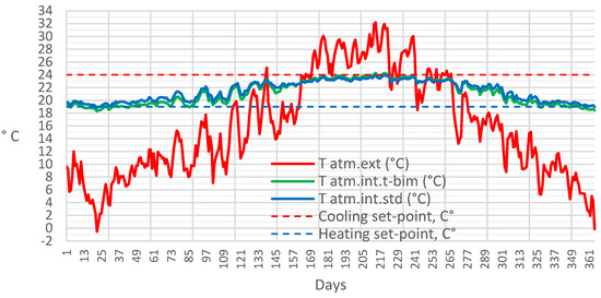
Figure 11.
Daily temperatures of indoor air in all zones are average according to the simulation results of the as-is STD and as-is T-BIM models and the average daily outdoor temperature of the typical meteorological year TMY 2007–2021 used in the simulations of both models.
3.3.1. Heating and Cooling Energy Demands
The different simulations of heat gains and losses for the same type of envelope element and their variables, that is, the Uvalues of glazing, external walls, and floors, as well as the infiltration rates, were used to calibrate the models. Calibration data also included the Uvalues that varied due to geometric and dimensional differences, especially in the size of the zones and the glazing. Figure 12 shows the recorded heat gains and losses.
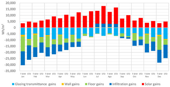
Figure 12.
Means of monthly average monthly energy gains obtained by energy simulations of the two models, as-is STD and as-is T-BIM, on a TMY 2007–2021.
There were differences between both models for solar gains through the glazing due to the different dimensions of the window panes. In the transmittances, even though the Uwin.pane was the same for both models, it must be taken into account that the as-is STD model presented the global value with the window frames, while the as-is T-BIM model was exclusively calculated with the Uvalue of the window panes.
The differences in annual heat losses between STD and T-BIM models through exterior walls and window glazing were −31.24 kWh/m2. The Uvalue differences for Uwall employed in each model (nominal calculation, in the as-is STD model; calculated with measurement parameters, in the T-BIM model) were not so high: 0.017 w/k·m2 higher in the T-BIM model. More notable were the heat losses to the ground. The temperature of the ground was the same for both models. However, the Ufloor value that determined the calibration process of the as-is T-BIM model was 0.466 w/km2 higher.
There was a similar indoor climate global thermal demand of 152 kWh/m2 for each model. However, the distribution of demand types was not the same, as the T-BIM model cooling energy demand was lower and represented 77% of the STD, while the T-BIM heating demand was significantly higher, at 161% of the STD model (Table 7).
Table 7.
Statistical simulation values for the as-is STD and the as-is T-BIM simulated models.
Comparing the monthly evolution of the thermal ambient conditioning demands (Figure 13), a similar behaviour was observed for each month, which is to say, a gradual change from cooling towards THE need for heating. There was a higher monthly energy demand for heating in the as-is T-BIM model toward the winter, and vice versa, a greater demand for air conditioning in the STD model toward the summer.
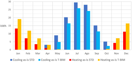
Figure 13.
Monthly demand for heating and cooling of the models, as-is STD and as-is T-BIM, in a TMY 2007–2021.
3.3.2. Heating and Cooling Energy Consumption
Given the results of the thermal conditioning energy demand (Table 7) and the characteristics of the air-conditioning services (Table 3), the annual air-conditioning energy consumption results, both in the as-is T-BIM and in the STD models, were low and very similar: 52.2 kWh/m2 and 53.5 kWh/m2, respectively. As with energy demand, there was an unequal distribution of consumption, with values of 26.3 kWh/m2 and 28.9 kWh/m2 for heating, and 16.3 kWh/m2 and 37.2 kWh/m2 for refrigeration, according to the simulation results of the as-is T-BIM and STD models, respectively.
In global terms of energy consumption and CO2 emissions, the differences determined by the use of the two methodologies, as-is STD and as-is T-BIM, are not significant in our case study. It is predictable that this will happen as long as the energy source for the heating and cooling systems of the buildings has yields and energy vectors similar to those in our case study.
3.3.3. User Comfort Conditions
PPD and PMV Fanger parameters were calculated based on the CFT simulation results with Energy Plus to evaluate user comfort. There are differences when comparing the results from both models: as-is STD and as-is T-BIM. In what follows, the results corresponding to the W1 zone and the 18, 19, and 20 November 3D-T scans are discussed. The room measurements were taken under the conditions described in Section 2.5.3, while the simulated weather conditions corresponded to the TMY 2007–2021. Although the room climate simulation conditions were different from 3D-T measurements, we considered that the solar radiation intensities were similar. In this way, the 3D-T model may facilitate the interpretation of the Fanger simulations, as solar radiation is a determining factor in the comfort of zone W1.
Figure 14 shows the hourly values of the Fanger PMV and PPD comfort parameters for zone W1, on 18–20 November of/ TMY 2007–2021. The hourly comfort values between 8:00 h and 20:00 h corresponding to the period of occupation of the room are depicted in graphs.
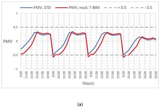
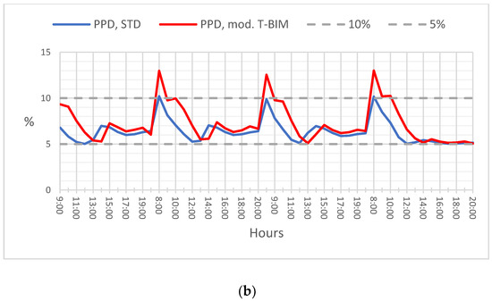
Figure 14.
Hourly values of Fanger comfort parameters for zone W1 on 18–20November of TMY 2007–2021: (a) PMV and (b) PPD.
Analysing the hourly values of PMV in Figure 14a, it can be seen that it stays within the comfort range, in other words, between (−0.5, +0.5), almost at all times. However, Figure 14b, shows the existence of peaks outside the comfort range, with PPD values > 10% in the early hours of the T-BIM model simulations.
The results of both models confirmed the permanence of values within the Fanger comfort intervals (see Section 2.4). The PMV and PPD are generic hourly indices for the prediction of comfort for the entire space obtained from the CTF simulation of the as-is T-BIM and STD models during the TMY month synchronised to the calibration period. CFD calculations of the performance of the air inside the W1 zone can yield detailed knowledge of the spatial distribution of these values. The tool in use generates images in stationary mode.
3.3.4. CFD Analysis of Spatial Distribution of Comfort in Room W1
The CFD tests were conducted with the two models, as-is STD and as-is T-BIM, as follows: The CDF module of DesignBuilder V6 and a spatial distribution of indoor air temperatures and air-flow speeds within zone W1, corresponding to each model for the same day of the month, were used. The time chosen to conduct the tests was 17:00 h on 19 November TMY 2007-21 to contrast those extreme discomfort values with the simulated values.
The criteria, which are set out below, were considered to establish the basis for the CFD calculations of each model. Steps were taken to set up approximate special calculation domain meshes, taking into account the small geometric differences that exist in each one (Figure 15). The CTF simulation results of each model were linked to the hour and day of the typical month of the year (17:00, 19 November TMY 2007–21) to determine the base contour parameters for the simulations of each model: as-is STD and as-is T-BIM. In Figure 16 and Table 8, the surface temperature and air flows of the CTF simulation are shown for the hour and day of the test and linked as contour values for the CFD simulations. The k-ε turbulence model was used for all the simulation calculations and the studies on the distribution of indoor air in thermal zones with low air circulation speeds [58]. The convergence of the calculations was produced with 6000 and 10,000 iterations in the as-is STD and as-is T-BIM models, respectively.

Figure 15.
Models of Room W1, domain mesh, air intake, and outtake vents in red (a) as-is STD and (b) as-is T-BIM. Where: Vent 1 is ventilation air intake; Clim 1–3 are climatized air intake diffusors; Inf 1–7 are infiltrations of air through the window frames; Ext 1–2 are air extractions from the air conditioning system and through the door access.
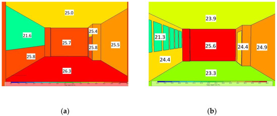
Figure 16.
Surface temperature values of contour elements linked for CFD simulation testing at 17:00 h on 19 November, in Room W1: (a) as-is STD and (b) as-is T-BIM.
Table 8.
Intake and outtake air flows of contour elements linked for the CFD trial simulation at 17 h on 19 November, in Room W1.
In Figure 17a,b, the 2D graph maps of the temperature distributions for the plane Z = 1.50 m of Zone W1 of both models are shown. Figure 18c illustrates the mapping of the point-to-point temperature differences, with the average of all those differences and the value of the statistical variance being 0.305 °C and 0.062 °C, respectively.
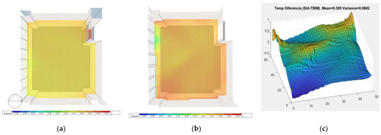
Figure 17.
Temperature value 2D graph maps on a horizontal plane at Z = 1.50 m, obtained by CFD simulation of air flows, according to the condition of Room W1, at 17 h, on 19NovemberTMY 2007–2021: (a) Temperatures with the as-is STD Model, (b) Temperatures with the as-is T-BIM Model, and (c) Point-to-point resolution of temperature differences between both models that were compared.
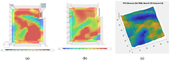
Figure 18.
2D graph maps of PPD comfort values on a horizontal plane at Z = 1.50 m, obtained by CFD simulation of atmospheric air flows, according to the conditions of Room W1, at 17 h, on 19 November TMY 2007–2021: (a) PPD of the as-is STD model; (b) PPD of the as-is T-BIM model; and (c) Point-to-point resolution of PPD differences in a comparison between both models.
Figure 18 and Figure 19 present the spatial mapping of PPD and PMV after processing of the CFD test results (temperature distribution and air-flow speeds within the zone) with the Fanger method for each of the models. The differences between the results of these two models were also statistically analysed in spatial terms through an evaluation of the temperature differences of each point on the Z = 1.50 plane and jointly through PPD and PMV values, respectively, and variances of the data sets. Averages of 0.739 and 0.039, and variance values of 3.82 and 0.14, for PPD and PVM, respectively, under the as-is STD and the as-is T-BIM model test conditions, were reported.
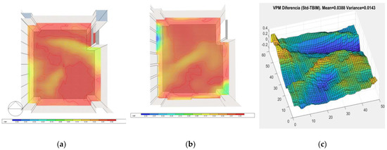
Figure 19.
2D graph maps of PMV comfort values on the horizontal plane at Z = 1.50 m, obtained by CFD simulation of atmospheric air flows, according to the conditions of Room W1, at 17 h, on 19NovemberTMY 2007–2021: (a) PMV of the as-is STD model; (b) PMV of the as-is T-BIM model; and (c) Point-to-point resolution of PMV differences in a comparison between both models.
The thermal sensations of occupants at different points within Room W1 can be quantified with the PPD and PMV values, in accordance with the test conditions. The PPD values tell us the percentage of dissatisfied people, a value that will always be >5% and never be negative. The information provided in Figure 18 shows the differences between the results of both models. The PPD indicator establishes a limit value of 10% between comfort and non-comfort. It may be appreciated that the results of the models point to higher intensities of the PPD value in approximately the same zones, with the results of the as-is STD model (Figure 18a) showing a wider distribution of PDD values, close to or greater than 10%, than the results of the as-is T-BIM model. The statistical results informed us that the difference was relatively small, given that the differences in the PPD value between both models were lower than 1% and 4% for the average and variance of the set of values, respectively. On the other hand, it can be understood from the sign of the PMV values whether the values of dissatisfaction are due to thermal intensities tending towards sensations of coldness or warmth because neutrality is situated around zero, limiting the comfort zone for office spaces to the interval (−0.5, +0.5). Analying the thermal images of both models, as-is STD and as-is T-BIM (Figure 19a,b), the total surface of the images with positive heat values is shown, with the thermal map of the as-is STD model presenting higher intensity values. In addition, it was the only map that, with values higher than +0.5 showed indicators of thermal dissatisfaction due to excessive heat. Although the as-is STD model values were over the limit values, the values of the as-is T-BIM model were close to that limit and approximately in the same places; therefore, the results can be considered similar. Neither did the statistical values point to numerically significant differences between the PMV values of both models, as-is STD and as-is T-BIM, because those differences were lower than +0.04 and 0.015 for the average and variance of the set of values, respectively.
4. Conclusions
This article reports a case study that successfully tests the as-is T-BIM method of building thermal information modelling. The goal of the as-is T-BIM method is to integrate multi-zone thermal point clouds into the as-is BEM procedures. Automatic time series processing of point clouds from five adjacent zones of a building created a proprietary semantic multi-zone as-is T-BIM model with time series of surface temperatures linked to each surface element of the model. This model has been automatically converted to a standard gbXML as-is BEM that has been used by conventional energy simulation software without interoperability errors. The novelty of the test case is the achievement of a clean scan for an as-is BEM workflow and the subsequent energy simulation of a multi-zone set without obtaining any interoperability errors. Furthermore, the temperature series corresponding to each of the classes of elements that conform to the thermal zones has made possible the aggregation of thermal transmittance values in the as-is BEM model.
The novelty of the as-is T-BIM method is the processing of 3D thermal clouds of interior zones of a building to generate a semantic multi-zone proprietary model that contains time series of surface temperatures assigned to its surface elements. This proprietary as-is T-BIM model has automatically generated a multi-zone gbXML as-is BEM for energy simulation.
A comparison of the simulation results obtained with T-BIM and conventional methods for the same building reveals shorter modelling times and more accurate geometric models. Although the overall energy simulation results of the two models are very close, there are differences in the heating and cooling energy demand profiles obtained for each of them. Although the availability of more experimental information for the calibration of the as-is T-BIM model suggests a higher accuracy for this model, in future studies it will be necessary to establish benchmarks to determine the thermal accuracy of this method. Nevertheless, the successful achievement of obtaining a multizone model automatically is a previous step to the multi-storey model that is necessary to address the complexity of a complete building. The multi-zone feature of the as-is T-BIM method makes it applicable to single-storey buildings, automating data acquisition and processing and improving the accuracy of energy simulation results.
The following future lines of research and development concerning as-is T-BIM technology have been established: the use of multi-storey as-is T-BIM models for the creation of standard BEM format files of complete buildings; greater control over the climatic conditions of the thermal scanner sessions to ensure the thermal temperature in the outdoor building environment and the in-door thermal zones that are suitable to reach the most appropriate conditions for the calculation of envelope element transmittances; validation of calibrated energy models using real building consumption data as AG14 recommends, and the use of the T-BIM method for studying indoor comfort conditions under as-is working environments.
Author Contributions
Conceptualisation, A.A.O., C.A.-F., J.-L.V.B. and V.P.-A.; methodology, A.A.O., C.A.-F., J.-L.V.B. and V.P.-A.; software, A.A.O. and V.P.-A.; validation, C.A.-F. and V.P.-A.; formal analysis, A.A.O., C.A.-F. and V.P.-A.; investigation, A.A.O., C.A.-F., J.-L.V.B. and V.P.-A.; writing—original draft preparation, V.P.-A.; writing—review and editing, A.A.O., C.A.-F., J.-L.V.B. and V.P.-A.; supervision, A.A.O., C.A.-F. and J.-L.V.B.; All authors have read and agreed to the published version of the manuscript.
Funding
This research was funded by the European Regional Development Fund (SBPLY/19/180501/000094 project) and the Ministry of Science and Innovation (PID2019-108271RB-C31 and PID2019-108271RB-C33).
Data Availability Statement
Not available.
Conflicts of Interest
The authors declare no conflict of interest.
Abbreviations
| 3D-T | Geometric point-cloud. |
| AG14 | Ashrae Guideline 14. |
| BEM | Building energy modelling. |
| BES | Building energy simulation. |
| CFD | Computational fluid dynamics. |
| CTF | Conduction transfer functions. |
| GBXML | Green building XML format. |
| IRT | InfraRed technology. |
| PMV | Predicted mean vote. |
| PPD | Predicted percentage dissatisfied. |
| T-BIM | Thermal building information modelling. |
References
- González-Torres, M.; Pérez-Lombard, L.; Coronel, J.F.; Maestre, I.R.; Yan, D. A review on buildings energy information: Trends, end-uses, fuels and drivers. Energy Rep. 2022, 8, 626–637. [Google Scholar] [CrossRef]
- United Nations Environment Programme. The 2020 Global Status Report for Buildings and Construction: Towards a Zero-Emissions, Efficient and Resilient Buildings and Construction Sector. Global Alliance for Building Construction, pp. 10–20. 2020. Available online: https://globalabc.org/resources/publications/2020-global-status-report-buildings-and-construction (accessed on 10 January 2023).
- Villena, F.; García, T.; Ballesteros, P.; Pellicer, E. Energy and environmental impact of the CTE-DB-HE evolution on a single-family house. In Proceedings of the 23rd International Congress on Project Management and Engineering, Málaga, Spain, 10–12 July 2019; Volume 29, pp. 1466–1480. [Google Scholar]
- Ministerio de Fomento, Gobierno de España. Documento Básico Ahorro de Energía, Código Técnico de la Edificación. 2013, 1–129.
- The Council of the European. Directive 2002/91/EC on the energy performance of buildings, 16 December 2002. Off. J. Eur. Communities 2003, 1, 1–7. [Google Scholar]
- Ramaji, I.J.; Messner, J.I.; Leicht, R.M. Leveraging building information models in IFC to perform energy analysis in openstudio®. ASHRAE IBPSA-USA Build. Simul. Conf. 2016, 6, 251–258. [Google Scholar]
- Elnabawi, M.H. Building Information Modeling-Based Building Energy Modeling: Investigation of Interoperability and Simulation Results. Front. Built Environ. 2020, 6, 1–19. [Google Scholar] [CrossRef]
- Gao, H.; Koch, C.; Wu, Y. Building information modelling based building energy modelling: A review. Appl. Energy 2019, 238, 320–343. [Google Scholar] [CrossRef]
- González, J.; Soares, C.A.P.; Najjar, M.; Haddad, A.N. Bim and bem methodologies integration in energy-efficient buildings using experimental design. Buildings 2021, 11, 491. [Google Scholar] [CrossRef]
- Gerrish, T.; Ruikar, K.; Cook, M.; Johnson, M.; Phillip, M. Using BIM capabilities to improve existing building energy modelling practices. Eng. Constr. Archit. Manag. 2017, 24, 190–208. [Google Scholar] [CrossRef]
- Negendahl, K. Building performance simulation in the early design stage: An introduction to integrated dynamic models. Autom. Constr. 2015, 54, 39–53. [Google Scholar] [CrossRef]
- Méndez Echenagucia, T.; Capozzoli, A.; Cascone, Y.; Sassone, M. The early design stage of a building envelope: Multi-objective search through heating, cooling and lighting energy performance analysis. Appl. Energy 2015, 154, 577–591. [Google Scholar] [CrossRef]
- Bracht, M.K.; Melo, A.P.; Lamberts, R. A metamodel for building information modeling-building energy modeling integration in early design stage. Autom. Constr. 2021, 121, 103422. [Google Scholar] [CrossRef]
- Cho, Y.K.; Ham, Y.; Golpavar-Fard, M. 3D as-is building energy modeling and diagnostics: A review of the state-of-the-art. Adv. Eng. Inform. 2015, 29, 184–195. [Google Scholar] [CrossRef]
- Chen, J.; Fang, Y.; Cho, Y.K. Performance evaluation of 3D descriptors for object recognition in construction applications. Autom. Constr. 2018, 86, 44–52. [Google Scholar] [CrossRef]
- Ham, Y.; Golparvar-Fard, M. Mapping actual thermal properties to building elements in gbXML-based BIM for reliable building energy performance modeling. Autom. Constr. 2015, 49, 214–224. [Google Scholar] [CrossRef]
- Wang, C.; Cho, Y.K.; Gai, M. As-is 3D Thermal Modeling for Existing Building Envelopes Using a Hybrid LIDAR System. J. Comput. Civ. Eng. 2013, 27, 645–656. [Google Scholar] [CrossRef]
- Demisse, G.G.; Borrmann, D.; Nüchter, A. Interpreting Thermal 3D Models of Indoor Environments for Energy Efficiency. J. Intell. Robot. Syst. Theory Appl. 2015, 77, 55–72. [Google Scholar] [CrossRef]
- Ramón, A.; Adán, A.; Castilla, A. Thermal point clouds of buildings: A review. Energy Build. 2022, 274, 112425. [Google Scholar] [CrossRef]
- Adán, A.; Prado, T.; Prieto, S.A.; Quintana, B. Fusion of thermal imagery and LiDAR data for generating TBIM models. In Proceedings of the 2017 IEEE SENSORS, Glasgow, UK, 29 October 2017; pp. 1–3. [Google Scholar]
- Adán, A.; Pérez, V.; Vivancos, J.L.; Aparicio-Fernández, C.; Prieto, S.A. Proposing 3D thermal technology for heritage building energy monitoring. Remote Sens. 2021, 13, 1537. [Google Scholar] [CrossRef]
- Prieto, A.; Quintana, B.; Adán, A.; Vázquez, A.S. As-is building-structure reconstruction from a probabilistic next best scan approach. Robot. Auton. Syst. 2017, 94, 186–207. [Google Scholar] [CrossRef]
- Vollmer, M.; Mollman, K.P. Infrared Thermal Imaging: Fundamentals, Research and Applications; WILEY-VCH: Hoboken, NJ, USA, 2017; p. 478. [Google Scholar]
- Dall’O’, G.; Sarto, L.; Panza, A. Infrared screening of residential buildings for energy audit purposes: Results of a field test. Energies 2013, 6, 3859–3878. [Google Scholar] [CrossRef]
- Bienvenido-Huertas, D.; Rodríguez-Álvaro, R.; Moyano, J.J.; Rico, F.; Marín, D. Determining the U-Value of fa ades using the thermometric method: Potentials and limitations. Energies 2018, 11, 360. [Google Scholar] [CrossRef]
- Nardi, I.; Sfarra, S.; Ambrosini, D. Quantitative thermography for the estimation of the U-value: State of the art and a case study. In Proceedings of the 32nd Italian Union of Thermo-Fluid-Dynamics, Pisa, Italy, 23–25 June 2014. [Google Scholar]
- Grinzato, E.; Vavilov, V.; Kauppinen, T. Quantitative infrared thermography in buildings. Energy Build. 1998, 29, 1–9. [Google Scholar] [CrossRef]
- Fokaides, P.A.; Kalogirou, S.A. Application of infrared thermography for the determination of the overall heat transfer coefficient (U-Value) in building envelopes. Appl. Energy 2011, 88, 4358–4365. [Google Scholar] [CrossRef]
- Tejedor, B.; Casals, M.; Gangolells, M.; Roca, X. Quantitative internal infrared thermography for determining in-situ thermal behaviour of façades. Energy Build. 2017, 151, 187–197. [Google Scholar] [CrossRef]
- European Standard EN ISO-7730:2005; Ergonomics of the Thermal Environment. Analytical Determination and Interpretation of Thermal Comfort Using Calculation of the PMV and PPD Indices and Local Thermal Comfort Criteria. ISO: Geneva, Switzerland, 2005.
- Blázquez, T.; Suárez, R.; Sendra, J.J. Hacia una calibración de modelos energéticos: Caso de estudio del parque residencial español en clima mediterráneo. Inf. Construcción 2015, 67, e128. [Google Scholar]
- Vrachimi, I.; Melo, A.P.; Cóstola, D. Prediction of wind pressure coefficients in building energy simulation using machine learning. In Proceedings of the Building Simulation 2017: 15th Conference of IBPSA, San Francisco, CA, USA, 7–9 August 2017. [Google Scholar]
- Ruiz, G.R.; Bandera, C.F. Validation of calibrated energy models: Common errors. Energies 2017, 10, 1587. [Google Scholar] [CrossRef]
- Shi, X.; Si, B.; Zhao, J.; Tian, Z.; Wang, C.; Jin, X.; Zhou, X. Magnitude, causes, and solutions of the performance gap of buildings: A review. Sustainability 2019, 11, 1–21. [Google Scholar] [CrossRef]
- American Society of Heating, Ventilating, and Air Conditioning Engineers (ASHRAE). Guideline 14-2014, Measurement of Energy and Demand Savings; Technical Report; American Society of Heating, Ventilating, and Air Conditioning Engineers: Atlanta, GA, USA, 2014. [Google Scholar]
- Efficiency Valuation Organization. International Performance Measurement and Verification Protocol: Concepts and Options for Determining Energy and Water Savings, Volume I; Technical Report; Efficiency Valuation Organization: Washington, DC, USA, 2012. [Google Scholar]
- Webster, L.; Bradford, J.; Sartor, D.; Shonder, J.; Atkin, E.; Dunnivant, S.; Frank, D.; Franconi, E.; Jump, D.; Schiller, S.; et al. M&V Guidelines: Measurement and Verification for Performance-Based Contracts; Version4.0, Technical Report; U.S. Department of Energy Federal Energy Management Program: Washington, DC, USA, 2015. [Google Scholar]
- Zhan, S.; Wichern, G.; Laughman, C.; Chong, A.; Chakrabarty, A. Calibrating building simulation models using multi-source datasets and meta-learned Bayesian optimization. Energy Build. 2022, 270, 112278. [Google Scholar] [CrossRef]
- Ji, L.; Shu, C.; Hou, D.; Laouadi, A.; Wang, L.; Lacasse, M. Predicting indoor air temperatures by calibrating building thermal model with coupled airflow networks. In Proceedings of the REHVA 14th HVAC World Congress, Rotterdam, The Netherlands, 22–25 May 2022; pp. 1–8. [Google Scholar]
- Baba, F.M.; Ge, H.; Zmeureanu, R.; Wang, L. (Leon) Calibration of building model based on indoor temperature for overheating assessment using genetic algorithm: Methodology, evaluation criteria, and case study. Build. Environ. 2022, 207, 108518. [Google Scholar] [CrossRef]
- Guo, J.; Liu, R.; Xia, T.; Pouramini, S. Energy model calibration in an office building by an optimization-based method. Energy Rep. 2021, 7, 4397–4411. [Google Scholar] [CrossRef]
- Bayomi, N.; Nagpal, S.; Rakha, T.; Fernandez, J.E. Building envelope modeling calibration using aerial thermography. Energy Build. 2021, 233, 110648. [Google Scholar] [CrossRef]
- UNE UNE-EN ISO 6946:2021; Componentes y Elementos para la Edificación. Resistencia Térmica y Transmitancia Térmica. Método de Cálculo. (ISO 6946:2017, Versión Corregida 2021-12). ISO: Geneva, Switzerland, 2021.
- Gobierno de España, Instituto Eduardo Torroja de Ciencias de la Construcción, Consejo Superior de Investigaciones Científicas, Ministerio Ciencia e Innovación. Catálogo Elem. Constr. CTE 2010, 3, 1–141.
- ISO 10456:2007; Building Materials and Products. Hygrothermal Properties. Tabulated Design Values and Procedures for Determining Declared and Design Thermal Values. ISO: Geneva, Switzerland, 2007.
- ISO 9869-1:2014; Thermal Insulation—Building Elements—In Situ Measurement of Thermal Resistance and Thermal Transmittance. Part 1: Heat Flow Meter Method. ISO: Geneva, Switzerland, 2014.
- Albatici, R.; Tonelli, A.M.; Chiogna, M. A comprehensive experimental approach for the validation of quantitative infrared thermography in the evaluation of building thermal transmittance. Appl. Energy 2015, 141, 218–228. [Google Scholar] [CrossRef]
- Albatici, R.; Tonelli, A.M. Infrared thermovision technique for the assessment of thermal transmittance value of opaque building elements on site. Energy Build. 2010, 42, 2177–2183. [Google Scholar] [CrossRef]
- European EN 13187:1998; Thermal Performance of Buildings—Qualitative Detection of Thermal Irregularities in Building Envelopes—Infrared Method (ISO 6781:1983 Modified). ISO: Geneva, Switzerland, 1998.
- Asdrubali, F.; D’Alessandro, F.; Baldinelli, G.; Bianchi, F. Evaluating in situ thermal transmittance of green buildings masonries—A case study. Case Stud. Constr. Mater. 2014, 1, 53–59. [Google Scholar] [CrossRef]
- Gobierno de España. Ministerio de Fomento Codigo Técnico de la Edificación. Documento de bases para la actualización del Documento Básico DB-HE. Doc. Bases Actual. Doc. Básico DB-HE 2016, 1–13. [Google Scholar]
- Gobierno de España REAL DECRETO 1027/2007, de 20 de julio, por el que se aprueba el Reglamento de Instalaciones Térmicas en los Edificios. Bol. Estado 2007, 35931–35984.
- Kottek, M.; Grieser, J.; Beck, C.; Rudolf, B.; Rubel, F. World map of the Köppen-Geiger climate classification updated. Meteorol. Zeitschrift 2006, 15, 259–263. [Google Scholar] [CrossRef]
- Gobierno de España, Ministerio de Industria, Instituto para la Diversificación y Ahorro de la Energía (IDAE). Guía Técnica de Condiciones Climáticas Exteriores de Proyecto; 2010, p. 123. Available online: https://www.idae.es/uploads/documentos/documentos_12_Guia_tecnica_condiciones_climaticas_exteriores_de_proyecto_e4e5b769.pdf (accessed on 10 January 2023).
- Mobaraki, B.; Komarizadehasl, S.; Castilla Pascual, F.J.; Lozano-Galant, J.A. Application of Low-Cost Sensors for Accurate Ambient Temperature Monitoring. Buildings 2022, 12, 1411. [Google Scholar] [CrossRef]
- Sensirion, A.G. Datasheet SHT3xA-DIS. Humidity, Automotive Grade Sensor, Temperature. 2019. Available online: https://sensirion.com/products/catalog/ (accessed on 10 January 2023).
- Adán, A.; Quintana, B.; Prieto, S.A. Autonomous mobile scanning systems for the digitization of buildings: A review. Remote Sens. 2019, 11, 306. [Google Scholar] [CrossRef]
- Cortés, M.; Fazio, P.; Rao, J.; Bustamante, W.; Vera, S. CFD modeling of basic convection cases in enclosed environments: Needs of CFD beginners to acquire skills and confidence on CFD modelling. Rev. Ing. Construcción 2014, 29, 22–45. [Google Scholar] [CrossRef]
Disclaimer/Publisher’s Note: The statements, opinions and data contained in all publications are solely those of the individual author(s) and contributor(s) and not of MDPI and/or the editor(s). MDPI and/or the editor(s) disclaim responsibility for any injury to people or property resulting from any ideas, methods, instructions or products referred to in the content. |
© 2023 by the authors. Licensee MDPI, Basel, Switzerland. This article is an open access article distributed under the terms and conditions of the Creative Commons Attribution (CC BY) license (https://creativecommons.org/licenses/by/4.0/).