Abstract
Exterior shading devices and outdoor units can be closely coupled since these two building components are commonly installed next to each other. This study uses a coupled EnergyPlus-Fluent modeling approach to examine how a combination of exterior shading and heat rejection from outdoor units can affect the ambient outdoor environment of a building, and how changes in the ambient outdoor environment can influence cooling loads and indoor PM2.5 exposure. Three exterior shading devices were simulated, including horizontal overhangs, vertical overhangs, and vertical fins. Data from wind-tunnel experiments and field measurements were used to ensure the accuracy of the airflow model, energy model, and pollution model developed in this study. Results indicate that horizontal overhangs could almost offset the increase in cooling loads due to increased ambient outdoor temperatures caused by heat rejection. The use of vertical overhangs did not always mean lower demand for space cooling when heat rejection was considered. Heat rejection, horizontal overhangs, and vertical overhangs could help reduce indoor PM2.5 exposure, while indoor air pollution was worse after the implementation of vertical fins. This study shows how exterior shading devices and outdoor units can be coupled to achieve better building energy efficiency and improved occupant health.
1. Introduction
Buildings in Hong Kong account for 90% of the total electricity consumption and generate a proportionate share of carbon emissions [1]. The energy used for space cooling is responsible for 34% of the electricity consumed by the building sector in 2020 and is expected to increase as a result of climate change and the urban heat-island effects [2]. Buildings interact with their ambient outdoor environments through the conductive and convective heat flux at exterior surfaces, solar and longwave radiation exchange, and sensible and latent heat transfer via infiltration and ventilation [3]. There is thus a strong connection between space-cooling energy consumption and ambient outdoor environmental conditions. Given the need to reduce building-related carbon emissions, studying the factors that can cause ambient outdoor environmental conditions (e.g., ambient outdoor temperature) to vary has increased as a research priority in the energy research community.
Many of today’s buildings in Hong Kong rely on a combination of split-type air conditioners and exterior shading devices for cooling. Split-type air conditioning is widely used because of its simplicity, low costs, ease of operations, and ability to provide individual control [4,5]. A split-type air conditioner is composed of an indoor unit and an outdoor unit. An outdoor unit rejects the heat that is absorbed by the indoor unit to the ambient outdoor environment of a building. The use of exterior shading devices is an important aspect of energy-efficient building design strategies, especially for buildings that are completely exposed to the sun [6,7]. Overhangs and vertical fins are the two most frequently occurring exterior shading devices in Hong Kong. Exterior shading devices can not only prevent unwanted solar heat gain from entering the indoor space but also act as a wind-blocking component to influence the pattern of the airflow around a building.
The effect of outdoor units or exterior shading devices on the ambient outdoor environment of a building has been examined in several studies. Chow and Lin [8] used a computer program to estimate temperatures of the air around the outdoor units installed in a building re-entrant and concluded that (1) heat rejection from the outdoor units of rooms on lower floors could increase the ambient outdoor temperatures of rooms on higher floors, and (2) this temperature increase resulted in a reduction in the energy efficiency of outdoor units and therefore caused an increase in space-cooling energy consumption. Hsieh et al. [9] examined how heat rejection from outdoor units affected the thermal environment outside a high-rise building and suggested that installing the outdoor units on every third floor helped slow down the increase in ambient outdoor temperatures caused by heat rejection. Han and Chen [10] evaluated the impact of the positions of outdoor units on the ambient outdoor temperatures of buildings and pointed out that outdoor units should be placed outside of building gaps to avoid the accumulation of heat in those gaps. In terms of exterior shading devices, a modeling study carried out by Cui et al. [11] indicates that overhangs had a significant impact on the pattern of the airflow within a street canyon, while vertical fins only had a minor impact. Research by Xiong and Chen [12] shows that the use of overhangs led to an increase in the speed of the air near windows. Zheng et al. [13] used a numerical method to analyze the characteristics of the airflow near the windows that were externally shaded by louvers and found that there was a significant variation in air exchange rates due to the vortexes produced between windows and louvers.
When examining the factors that influence the ambient outdoor environment of a building, previous studies have focused on either outdoor units or exterior shading devices. There has been significantly less research into the effect that a combination of outdoor units and exterior shading devices can have on the ambient outdoor environment of a building, even though the two building components are frequently installed next to each other. The temperature of the hot air from outdoor units is highly dependent on cooling loads [14]. The role of exterior shading devices in reducing cooling loads, therefore, means that outdoor units and exterior shading devices can be closely correlated. Additionally, both exterior shading devices and heat rejection from outdoor units can influence the pattern of the airflow around a building, indicating the importance of considering the potential interaction between exterior shading devices and outdoor units when examining the pattern of the airflow around a building.
Indoor air quality is also highly correlated with the ambient outdoor environment of a building. Air pollutants from the ambient outdoor environment can infiltrate into a building through cracks in the externally exposed facades (the walls, roof, and ground floor) and, if open, windows. Exposure to air pollutants has been associated with some negative health effects. For instance, an epidemiological study [15] shows that exposure to high levels of fine particles (also known as PM2.5) could cause about 3% of all mortality from cardiopulmonary disease and around 1% of mortality from acute respiratory infections in children under age five.
As the level of ambient outdoor air pollution acts as an important modifier in exposure to indoor air pollutants, many studies have been carried out to look at the characteristics of ambient outdoor air pollution. Keshavarzian et al. [16] used a tracer gas technique to measure the time-dependent air pollutant concentrations around a building and found that air pollutants were trapped in the building’s wake for a long time. Ng and Chau [17] evaluated the effectiveness of different configurations for two building design elements in reducing air pollution in isolated deep street canyons. Cui et al. [11] investigated the effects of exterior shading devices on pollutant dispersion within urban street canyons. Meng et al. [18] used computational fluid dynamics (CFD) simulations to study the distribution of PM2.5 concentrations around buildings in a traffic-intensive area and concluded that the concentrations of PM2.5 near rooms on 17th or higher floors remained stable. A delicate CFD research of a multi-street canyon model with non-uniformities of buildings was carried out by Wen et al. [19] to investigate the dispersion of pollutants between compact urban blocks. There have also been field studies [20,21,22] measuring the levels of ambient outdoor air pollutants of buildings with roadside, urban, and rural locations, and modeling studies [23,24,25] indicating that the ground-, middle-, and top-floor flats in high-rise residential buildings saw different ambient outdoor air pollutant concentrations.
Although previous studies have investigated how ambient outdoor pollutant concentrations were affected by factors such as the building geometry, building elements, building height, and location, there are sparse data describing how a combination of exterior shading devices and heat rejection from outdoor units can influence ambient outdoor air pollutant concentrations. In Hong Kong, most outdoor units blow hot air directly into the ambient outdoor environment of a building. The flow of the hot air from outdoor units is expected to cause changes in the pattern of the airflow around a building and thus affect the distribution of ambient outdoor air pollutants. The presence of exterior shading devices can block the flow of the hot air or make the hot air flow in different directions.
The research presented here investigates how a combination of exterior shading devices and heat rejection from outdoor units can affect the ambient outdoor environmental conditions (including ambient outdoor temperatures and ambient outdoor PM2.5 concentrations) of a six-story building in Hong Kong, and examines variations in building performance (including cooling loads and exposure to indoor PM2.5) due to changes in ambient outdoor environmental conditions. EnergyPlus [26], an open-source whole-building energy modeling tool, was used to calculate cooling loads and indoor PM2.5 exposure concentrations of the building. Fluent [27], a fluid simulation tool, was used to model the airflow around the building. Cooling was modeled to a 25 °C set-point during occupied hours. The building was modeled in two different directions, in which case the outdoor units were either on the windward side or leeward side of the building. Three types of exterior shading devices were considered, including horizontal overhangs, vertical overhangs, and vertical fins. The outcomes of this study can lead to a better understanding of the interactions between outdoor units, exterior shading devices, and ambient outdoor environments, as well as provide an insight into how exterior shading devices and outdoor units can be coupled to improve both building energy efficiency and indoor air quality.
2. Methods
2.1. Building Physics Models
Building physics models of a city block that was typical in Hong Kong were developed in this study. The city block (Figure 1a) was composed of nine six-story office buildings, which were arranged in a 3 × 3 array. All the buildings had the same built form, size, and construction materials. The width of individual street canyons was 10 m. The building in the center of the city block was the target building. Buildings surrounding the target building were unoccupied and were modeled as blocks that provided shading and blocked winds. The target building was modeled at two orientations (North or South). Each floor of the target building, except for the ground floor, had an open-plan room (ceiling height: 3.4 m; floor area: 80 m2) with a north- or south-facing window (width: 7.0 m; height: 1.8 m). The window-to-wall ratio for each room was 0.4. An outdoor unit was installed right below the window of individual rooms (Figure 1a). The ground-floor space and the space containing stairs and lifts (Figure 1b) were excluded from the analysis. There was a net heat flow of zero between any two adjacent rooms, between the bottom-floor room (i.e., room 1) and ground-floor space, or between rooms and the space containing stairs and lifts. Model inputs, including environment data, fabric characteristics, occupancy schedules, internal gains, air conditioning, ventilation, and shading strategies, are described below.

Figure 1.
(a) The city block; (b) The cross-section of the target building; (c) The vertical measurement lines, street, and vehicles outside the target building; (d) The surface for contours and vectors.
2.1.1. Environment Data
Weather data were taken from the climatological database maintained by the Hong Kong Observatory (HKO) [28]. Data about the background concentrations of outdoor PM2.5 were taken from the air quality database maintained by the Environmental Protection Department (EPD) [29]. Simulations were run for a period of three days when the target building relied on a combination of air conditioning and natural ventilation through open windows for cooling. Simulation results for day three were presented in Section 3, while the first two days were run to capture the thermal storage effect of building fabrics. The environment data for day three can be seen in Figure 2. As winds blew from the south for most of the time, the south winds were simulated for simplicity.
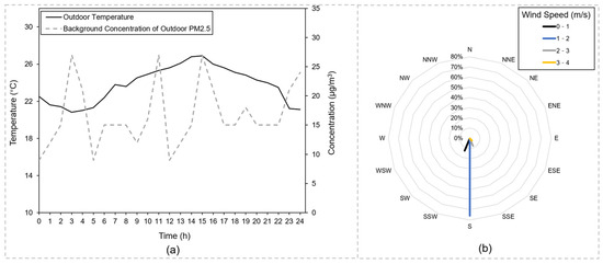
Figure 2.
(a) The outdoor temperatures and background concentrations of outdoor PM2.5 for day three; (b) The wind rose for day three.
2.1.2. Fabric Characteristics
The materials and thermal properties of building fabrics (Table 1) were determined based on a city-wide survey conducted in Hong Kong [30]. Data about the U-value of building fabrics and the thermal conductivity of fabric materials were taken from the Building Environmental Assessment Method (BEAM) Plus tables [31] and Buildings Department (BD) tables [32], respectively. The U-value of each building fabric was modified by adjusting the thicknesses of fabric materials. It should also be noted that thermal insulation is seldom applied to building fabrics in Hong Kong [33]. Building airtightness was modeled by applying a permeability, which is the air leakage rate per hour at an indoor-outdoor pressure difference of 50 Pa to building fabrics. An estimate of the building infiltration rate was made following the methodology outlined in ISO 13790 [34]. The building infiltration rate was then converted to a permeability of 11.5 m3/h/m2, using the volume and surface area of the building. A permeability was used rather than an infiltration rate to account for the variation in infiltration rates due to changes in wind pressures.

Table 1.
The building fabric types, fabric materials, and thermal properties.
2.1.3. Occupancy Schedules and Internal Gains
Occupancy schedules determine both internal gain patterns and period of exposure to indoor PM2.5. The number of occupants in each room was 7, consistent with the design occupation density for offices [35]. Each room was assumed to be occupied from 09:00 to 18:00. Data on internal gains were taken from CIBSE tables, including occupant gains (130 W per person, reflecting heat emissions from an average adult male who is doing very light work), lighting gains (12 W/m2, reflecting the lighting loads for a maintained illuminance level of 500 lux), and equipment gains (15 W/m2, reflecting internal heat gains from small power office equipment) [35]. Occupant exposure to indoor PM2.5 was determined by overlaying the occupancy profile on the indoor PM2.5 concentration profile.
2.1.4. Air Conditioning, Ventilation, and Shading
The air-conditioning system of individual rooms was modeled as a split-type air conditioner. Each room was cooled to a set-point of 25 °C during occupied hours. Based on a manufacturer’s engineering data [36], specifications of the split-type air conditioner were as follows: (1) the coefficient of performance (COP) was 3.1; (2) the areas of the air inlet and air outlet of the outdoor unit were 1.1 m2 and 0.9 m2, respectively; and (3) the airflow rate of the outdoor unit was 65 m3/min. According to [37], the rate of heat rejection from an outdoor unit was calculated by adding cooling loads and the power consumption of the air conditioner. The temperature of the hot air from an outdoor unit was determined based on the following equation [14]:
where is the rate of heat rejected by the outdoor unit (); is the airflow rate of the outdoor unit (); is the specific heat of air (); and is the temperature of the air at the air inlet of the outdoor unit (°C).
The window in each room was closed during the entire simulation period. According to information provided in the BD database [32], three types of exterior shading devices were modeled, including horizontal overhangs, vertical overhangs, and vertical fins. The modeled exterior shading devices cover the exterior shading devices that are applied to more than 90% of the office buildings in Hong Kong [38]. The dimensions and schematic of individual exterior shading devices can be seen in Figure 3. It should be noted that in practice many overhangs have louvers that can swing open or closed. For simplicity, the overhangs modeled in this study were assumed to have all the louvers closed. In addition to the shading strategy that no shading was assigned to the building, there were four shading strategies in total (Table 2).
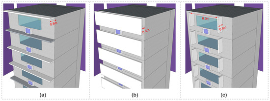
Figure 3.
(a) The schematic and dimensions of horizontal overhangs; (b) The schematic and dimensions of vertical overhangs; (c) The schematic and dimensions of vertical fins.
Table 2.
The four shading strategies.
2.2. Simulations
Building physics models of the city block described in Section 2.1 were constructed using EnergyPlus (version 22.1) and Fluent (version 2021-r1). EnergyPlus was used to estimate cooling loads based on a heat balance equation, analyze the characteristics of the airflow inside the building using a validated AirflowNetwork module, and estimate indoor PM2.5 concentrations based on a generic contaminant transport algorithm. Fluent was used to analyze the characteristics of the airflow around the building based on the governing equations for incompressible turbulent flow, and estimate outdoor PM2.5 levels using a stochastic tracking method. The EnergyPlus model and Fluent model were coupled using a quasi-dynamic coupling method, to improve the quality of model inputs (including ambient outdoor temperatures, ambient outdoor PM2.5 levels, temperatures of exterior surfaces, and wind pressure coefficients). Details of the EnergyPlus model, Fluent model, and coupled model are described below.
2.2.1. EnergyPlus Model
The EnergyPlus model calculated temperatures of exterior surfaces, cooling loads, and indoor PM2.5 levels at 10-min intervals and output these variables hourly.
Temperatures of exterior surfaces were calculated according to the following heat balance equation for exterior surfaces [12]:
where is the absorbed direct and diffuse solar radiation heat flux (); is the net long wavelength radiation flux exchange with the outdoor air and surroundings (); is the convective flux exchange with the outdoor air (); and is the conduction heat flux into the building envelope ().
Cooling loads were calculated according to the following heat balance equation for indoor air [10]:
where is the solar radiation heat gain (); is the radiation heat transfer from interior surfaces (); is the heat gain from ventilation (); is the heat gain from infiltration (); is the heat gain from conduction through building fabrics (); is the heat gain from occupants, lighting, and equipment (); and is the cooling load ().
Indoor PM2.5 concentrations from outdoor sources were simulated using a generic contaminant transport algorithm. The transient air mass equation for the change in generic contaminant concentrations of a zone can be expressed as follows [39]:
where is the generic contaminant storage term in zone air (kg/s); is the concentration of generic contaminants at the current time step (kg/m3); is the generic contaminant capacity multiplier; is the sum of internal generic contaminant loads from indoor sources; is the sum of removal rate from indoor sinks (kg/s); is the transfer of generic contaminants due to inter-zone air mixing (kg/s); is the concentration of generic contaminants in the zone air being transferred into this zone (kg/m3); is the transfer of generic contaminants due to infiltration and ventilation of outdoor air (kg/s); is the concentration of generic contaminants in outdoor air (kg/m3); is the transfer of generic contaminants due to system supply (kg/s); is the air system supply mass flow rate (kg/s); is the concentration of generic contaminants in the system supply airstream (kg/m3); is the transport of generic contaminants through diffusion between zone air and interior surfaces; and is the generic contaminant generation or removal rate as a function of zone air generic contaminant level at the previous time step.
Outdoor sources of PM2.5 included vehicles and the background concentrations of outdoor PM2.5 measured by EPD (described in Section 2.1.1). Based on a study of pollution from road traffic [18], the mass flow rate of PM2.5 from vehicles on the centerline of the street (Figure 1c) was set as kg/s. The infiltration of outdoor air was modeled through cracks in the building envelope (the external walls and roof). Internal walls, ceilings, and floors were also given cracks, allowing for the transfer of PM2.5 from one room to another. Cracks were assigned reference air mass flow coefficients according to the building permeability and surface area, and the air mass flow exponents were set as 0.66 [40]. The penetration factor, which is the fraction of PM2.5 lost due to deposition in the cracks as it enters the building, was assumed to be 0.8 [41]. The deposition rate for indoor PM2.5 was set as 0.19 h−1 [42].
2.2.2. Fluent Model
The Fluent model outputs ambient outdoor temperatures, ambient outdoor PM2.5 levels, and wind pressure coefficients. Data about the ambient outdoor environmental conditions were taken from the grid layer adjacent to the exterior surfaces of the building.
The standard k-ε method, which has been widely adopted in similar studies due to its accuracy and low computational costs [43,44], was used to model the flow field. As in previous studies [11,13], the flow of air was numerically stable and was thus treated as an incompressible flow. The governing equation for incompressible flow can be written in a general form as follows [13]:
where is the scalar, such as the velocity ingredient, turbulent kinetic energy, or dissipation rate; is the mean velocity; is the effective diffusion coefficient; and is the source term.
The pressure-velocity coupling was solved by the semi-implicit pressure-linked equation (SIMPLE) algorithm. All the equations were discretized using a second-order upwind method, except for the pressure equation, which was discretized using a second-order method. A standard function was used in the wall treatment. The time step used in simulations was one second. In each time step, the maximum number of iterations was 800. At the end of each time step, convergence was achieved with the scaled residuals being for the continuity equation and for the rest equations.
The dispersion of outdoor PM2.5 due to turbulence was predicted using a stochastic tracking model, which predicts the trajectory of a particle by integrating the force balance on the particle. The force balance equation can be written as follows [18]:
where is the air velocity; is the particle velocity; is the drag force per unit particle mass; is the gravitational acceleration; is the particle density; is the air density; and is the additional acceleration term.
The position of a particle was determined based on a report that contained information about the step-by-step trajectories of particles. The mass concentration was calculated based on the particle-in-the-box method, which can be written as follows [45]:
where is the mass of individual particles; is the particle in the sampling box; and is the volume of the sampling box.
The computational domain of the flow filed can be seen in Figure 4. The distance between the city block and each boundary was determined following the recommendations of COST [46] and AIJ [47]. To match the sizes of the models used in validation, the computational domain was scaled down at a ratio of 1:25. The independence of the Reynolds number () needs to be checked when constructing a reduced-scale model [48]. Simulation results indicate that the values of were approximately at the height of the building and approximately around outdoor units and exterior shading devices, meeting the independence requirement (i.e., ) [48].
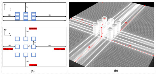
Figure 4.
(a) The dimensions of the computational domain; (b) The meshes drawn for the flow field.
To ensure accuracy and reduce computational costs, dense structured grids were drawn inside the city block (especially in the proximity of the building envelope, outdoor units, and exterior shading devices) while coarse structured grids were drawn outside the city block (Figure 4b). The height of the first grid layer adjacent to the exterior surfaces of the building, outdoor units, exterior shading devices, and the ground was 0.001 m, resulting in a mean y* of around 67. The mean y* met the requirement for high-quality meshing [49]. The growth ratio of continuous cells was kept below 1.2 to maintain a smooth transition in grid size.
A grid sensitivity analysis was conducted for 90 data points on the measurement lines outside the building (Figure 1c), to ensure that the model outputs (including the normalized wind velocity and normalized outdoor PM2.5 levels) were not influenced by grid size. Multiple modeling studies [50,51] have suggested a root-mean-square error (RMSE) of no greater than 10% as the independence requirement of grid size. The value of RMSE can be calculated based on the following equation [50]:
where and are the model outputs for the same data point under two different grid sizes, and is the total number of data points.
Three types of grids (including coarse grids, basic grids, and fine grids) were tested, where the refinement ratio was set as 1.1 following the recommendations from COST. The number of cells of the grids drawn for each shading strategy can be seen in Table 3, along with the calculated values of RMSE. Comparisons between different types of grids indicate that the coarse and basic grids had a RMSE of more than 20% while the basic and fine grids had a RMSE of less than 10%. The basic grids were considered to be an acceptable grid size and were used to conduct the validation and parametric studies.
Table 3.
The number of cells of the grids drawn for each shading strategy, along with the RMSE results.
2.2.3. Coupled EnergyPlus-Fluent Model
A quasi-dynamic coupling approach was used to couple the EnergyPlus model and Fluent model detailed in Section 2.2.1 and Section 2.2.2. The aim of this coupling was to improve the quality of model inputs. As described in Section 2.2.1, the EnergyPlus model was used to calculate cooling loads and indoor PM2.5 levels. The Fluent model could not calculate cooling loads, and it could not accurately estimate indoor PM2.5 levels due to the lack of ability to simulate the deposition of indoor PM2.5 onto interior surfaces. The accuracy of EnergyPlus outputs was highly dependent on three key inputs, including ambient outdoor temperatures, ambient outdoor PM2.5 levels, and wind pressure coefficients. As described in Section 2.2.2, the Fluent model could give accurate estimates of these three key inputs.
The data exchange between these two models was facilitated by a bespoke code written in MATLAB [52]. A schematic of the coupling approach can be seen in Figure 5. The EnergyPlus model was first run with the environment data file detailed in Section 2.1.1, estimating exterior surface temperatures and heat rejection rates. Then the Fluent model was run with the calculated exterior surface temperatures and heat rejection rates, estimating ambient outdoor temperatures, ambient outdoor PM2.5 levels, and wind pressure coefficients. It should be noted that the ambient outdoor temperatures or ambient outdoor PM2.5 concentrations of a room were determined by averaging the temperatures or concentrations of the cells adjacent to the exterior surfaces of the room. Finally, the EnergyPlus model was run with an environment data file that was modified to reflect the calculated ambient outdoor environmental conditions, estimating cooling loads, indoor PM2.5 levels, exterior surface temperatures, and heat rejection rates. The data exchange process took place at the beginning of each hour of the simulation period.

Figure 5.
The coupled simulation of EnergyPlus and Fluent.
The accuracy of the coupled EnergyPlus-Fluent model was governed by the similarity between the model inputs of EnergyPlus and those of Fluent. The same building geometrics were used in the EnergyPlus model and Fluent model. Additionally, these two models had the same boundary conditions. Boundary conditions of the Fluent model can be seen in Table 4.
Table 4.
Boundary conditions of the Fluent model.
The vertical profiles of wind speed () and temperature () described in Table 4 were determined using the same methods that EnergyPlus uses to estimate local outdoor temperatures and wind speeds. The vertical profile of wind speed was determined based on the following equation [44]:
where is the wind speed measured at the meteorological station (); is the boundary layer thickness of the wind speed profile at the meteorological station (); is the height of the station’s wind speed sensor above the ground (); is the exponent of the wind speed profile at the meteorological station; is the altitude; is the boundary layer thickness of the wind speed profile at the site; and is the exponent of the wind speed profile at the site.
The vertical profile of temperature was determined based on the following equation [44]:
where is the air temperature gradient (); is the radius of the Earth; is the altitude; is the offset equal to zero for the troposphere; and is the air temperature at the ground level for the troposphere (). was determined based on the following equation [44]:
where is the outdoor temperature measured at the meteorological station (); and is the height of the station’s wind speed sensor above the ground ().
The vertical profile of the turbulence kinetic energy () described in Table 4 was determined based on the following equation [47]:
where , , or is the root mean square of wind speed in the x-axis, y-axis, or z-axis direction at an altitude of ; and is the root mean square of streamwise wind speed at an altitude of .
The vertical profile of the turbulence dissipation rate () described in Table 4 was determined based on the following equation [47]:
where is the dimensionless k-ε model constant; and is the reference wind speed at a reference height of ().
2.3. Validation of Models
The EnergyPlus model and Fluent model were validated for accuracy in analyzing the characteristics of the flow field around buildings, levels of ambient outdoor pollutants, space-cooling energy consumption, and levels of indoor pollutants. It should be noted that the validation of the Fluent model was carried out using the grid size that was selected based on the grid sensitivity analysis conducted in Section 2.2.2.
2.3.1. Validation of the Flow Field around Buildings
The Architectural Institution of Japan (AIJ) [47] provided data on the velocities of the air in a wind tunnel. A city block composed of nine cubes with the same dimensions (length: 0.2 m; width: 0.2 m; height: 0.2 m) was placed in the wind tunnel (Figure 6). The width of individual street canyons was 0.2 m. Based on the recommendations from COST and AIJ [46,47], a computational domain was developed for the wind tunnel using Fluent. The height of the first near-wall grids on the exterior surfaces of cubes and the ground was 0.003 m, leading to a mean y* of approximately 98. The boundary conditions of the Fluent model were the same as the ones of the wind-tunnel test.
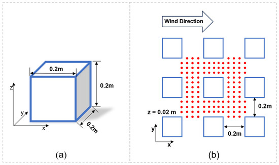
Figure 6.
(a) The dimensions of the cube; (b) The arrangement of cubes and measurement points.
A total of 120 measurement points (Figure 6b) were placed at a height of 0.02 m above the ground to measure the velocities of winds within the street canyons. The wind velocity was normalized by dividing the velocity value () by the inflow velocity at the same height (). Results for the measured and simulated normalized wind velocities can be seen in Figure 7, which indicates that the simulated wind velocities were generally in agreement with the measured ones. Large discrepancies were observed for the data points close to blocks. This was primarily due to the well-known weakness of the selected turbulent model in representing the turbulent kinetic energy in the layers adjacent to solid surfaces [53].
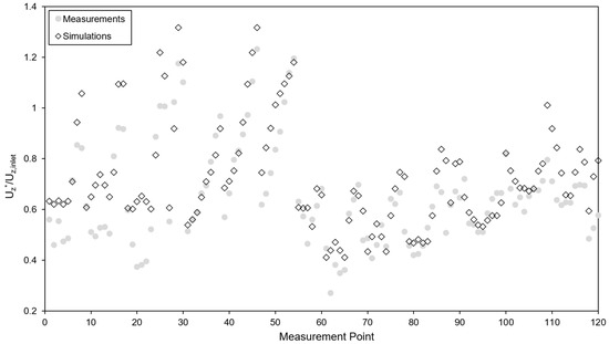
Figure 7.
The comparison of the measured and simulated normalized velocity for each measurement point.
The accuracy of the Fluent model was further checked according to three dimensionless metrics, including the fractional mean bias (FB), the factor of 2 of observations (FAC2), and normalized mean square error (NMSE). These dimensionless metrics were calculated based on the following equations [50]:
where n is the total number of data points; is the index of a data point; is the measured value of the data point; is the simulated value of the data point; and is the allowable absolute difference, which was set as 0.05 [54].
As in previous studies [55,56], the criteria for a Fluent model that provides reliable estimates for urban environmental conditions were , , and . Results indicate that the values of FB, FAC2, and NMSE for the Fluent model developed in this section were −0.1, 1, and 0.03, respectively, meeting the criteria. Therefore, the turbulent model and numerical settings adopted in this study can be used to accurately estimate the characteristics of the airflow within a city block.
2.3.2. Validation of Ambient Outdoor Pollutant Levels
The Meteorological Institute of the University of Hamburg [57] provided data about the dispersion of air pollutants in a wind tunnel. A city block composed of rectangular blocks with the same dimensions (length: 0.15 m; width: 0.10 m; height: 0.125 m) was placed in the wind tunnel (Figure 8). The width of individual street canyons was 0.1 m. Following the recommendations from COST and AIJ [46,47], a computational domain was developed for this wind tunnel using Fluent. The height of the first near-wall grids on the exterior surfaces of blocks and the ground was 0.002 m, leading to a y* of around 83. The boundary conditions of the Fluent model were the same as the ones of the wind-tunnel test. The pollutants were emitted at an overall rate of 0.1 m/s from four sources placed at the bottom of the emission block (Figure 8a), with the total emission area being 4.6 cm2.
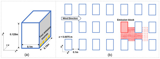
Figure 8.
(a) The dimensions of the emission block; (b) The arrangement of blocks and measurement points.
A total of 437 measurement points (Figure 8b) were placed at a height of 0.0075 m above the ground, measuring the concentrations of pollutants within the street canyons. The measured pollutant concentration was normalized to a dimensionless K value, which can be written as follows:
where is the measured pollutant concentration (ppm); is the reference wind speed measured at a height of 0.66 m above the ground (m/s); is the block height (m); is the concentration of pollutants at the source (ppm); and is the overall emission rate of pollutants (m3/s).
Results for the measured and simulated normalized pollutant concentrations can be seen in Figure 9, which indicates that the simulation results were generally consistent with the measured results. The comparisons also show that pollutant concentrations of the data points close to solid surfaces were overestimated due to the overprediction of turbulence dissipation (described in Section 2.3.1). The similarity between simulated and measured results was also demonstrated by the values of FB, FAC2, and NMSE being −0.1, 1, and 0.2, respectively. Therefore, the turbulent model, pollutant dispersion model, and numerical settings adopted in this study can be used to accurately estimate the concentrations of air pollutants within a city block.
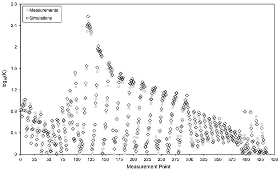
Figure 9.
The comparison of the measured and simulated normalized pollutant concentrations for each measurement point (the normalized pollutant concentration is expressed in log scale since there are some rapid changes in concentrations compared to the source strength).
2.3.3. Validation of Energy Use for Space Cooling and Indoor Pollutant Concentrations
A field measurement that was carried out for a main bedroom in a typical flat in Hong Kong (Figure 10a) provided data about space-cooling energy consumption and indoor pollutant concentrations. Fabric characteristics of the flat were as follows: (1) U-values of the external walls, roof, ground floor, and windows were 3.1 W/m2K, 0.42 W/m2K, 0.54 W/m2K, and 4.6 W/m2K, respectively; (2) the solar heat gain coefficient (SHGC) of the window glass was 0.76; and (3) the building permeability was 10.1 m3/h/m2 at an indoor-outdoor pressure difference of 50 Pa. No one was in the flat during the entire measurement period. Windows and internal doors were closed. The main bedroom was cooled to a temperature of 24 °C. The COP of the air conditioner in the main bedroom was 2.4.
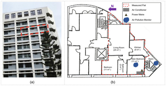
Figure 10.
(a) The measured main bedroom in a typical Hong Kong flat; (b) The indoor layout of the flat.
Measurements were carried out during the period from 28 to 30 September 2017. A portable power meter (SP2; BroadLink, Hangzhou, China) was used to measure the electricity consumed by the air conditioner in the main bedroom. The concentrations of indoor and outdoor PM2.5 were measured using two calibrated air pollution monitors (DUSTTRAK 8530 EP; TSI, Shoreview, MN, USA), which could measure a concentration up to 150 mg/m3 and had accuracy within ±5% of the actual results. One monitor was put in the main bedroom to measure indoor pollution levels, and the other was put on the outdoor stairs next to the main bedroom to measure outdoor pollution levels (Figure 10b). Data about the weather conditions were taken from a meteorological station close to the flat.
Two metrics, including the normalized mean bias error (NMBE) and the coefficient of variation of the root-mean-squared error (CVRMSE), were used to assess the similarity between the results of measurements and simulations. NMBE and CVRMSE were determined based on the following equations [58]:
where is the number of data points; is the index of a data point; is the measured value of the data point; is the simulated value of the data point; and is the average of measurements. To ensure the similarity between the two datasets, ASHRAE Guideline 14-2014 [58] suggests that the requirements of and should be met.
The EnergyPlus model was developed using the built form, fabric characteristics, occupancy, air conditioning, weather, and outdoor air pollution concentrations detailed above. The results of measurements and simulations for 29 September 2017 can be seen in Figure 11. The simulated electricity use of air conditioning was consistent with the measured one. This conclusion was further demonstrated by the low values of NMBE (4.5%) and CVRMSE (7.3%). In terms of indoor PM2.5 levels, the simulation results agreed with the measurement results. The values of NMBE and CVRMSE were 8.5% and 10.2%, respectively, meeting the ASHRAE Guideline 14-2014 requirements. Therefore, the AirflowNetwork module, contaminant transport algorithm, and numerical settings adopted in this study can be used to accurately estimate the space-cooling energy use and indoor pollutant concentrations of a building.
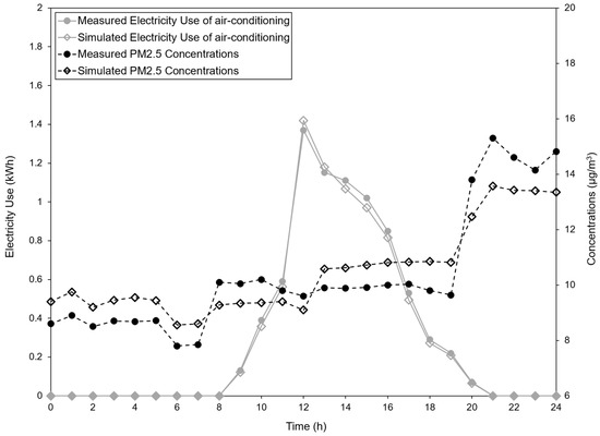
Figure 11.
Comparisons between the results of measurements and simulations for the electric energy use of air conditioning and indoor PM2.5 levels.
3. Results
This section presents the results of the ambient outdoor environmental conditions (including ambient outdoor temperatures, ambient outdoor PM2.5 levels, and airflow patterns), cooling loads, and indoor PM2.5 exposure concentrations of the target building operating under different shading strategies. The velocity vector and the contours of temperatures and pollutant concentrations for a selected surface in the computational domain (Figure 1d) were used as explanations for the results. To estimate changes in the ambient outdoor environment caused by exterior shading devices and heat rejection from outdoor units, as well as the resulting changes in cooling loads and indoor PM2.5 exposure, a reference case with no exterior shading devices and no heat rejection from outdoor units was simulated. The building was modeled in two directions. The windward scenario means that outdoor units were on the windward side of the building, while the leeward scenario means that outdoor units were on the leeward side of the building.
3.1. Ambient Outdoor Temperature
The changes in ambient outdoor temperatures due to exterior shading devices and heat rejection from outdoor units were averaged over the occupied hours (09:00 to 18:00) and are shown in Figure 12, where the positive value means an increase in ambient outdoor temperatures compared to the reference case.

Figure 12.
The changes in ambient outdoor temperatures of individual rooms caused by exterior shading devices and heat rejection from outdoor units.
3.1.1. Windward Scenario
Results for Strategy 1 support the conclusion of other studies [5,9] that the building experienced an increase in ambient outdoor temperatures when heat rejection from outdoor units was taken into account (Figure 12a). Different rooms showed a range of increases in ambient outdoor temperatures caused by heat rejection, from 0.1 °C to 1.1 °C. Room 2 experienced the largest increase in ambient outdoor temperatures. This result can be explained by the pattern of the airflow outside the building (Figure 13a). The hot air from outdoor units rose because it was less dense than the surrounding air, while winds flowed in the opposite direction. The conflict between the upward movement of hot air and the downward movement of winds limited the movement of heat and caused the accumulation of heat in the second-floor level of the street canyon. Room 5 experienced the smallest increase in ambient outdoor temperatures because most of the heat rejected by the outdoor unit of Room 5 was carried by winds to the lower part of the street canyon (Figure 13a).
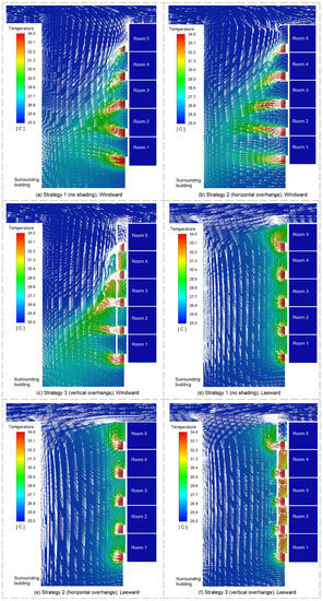
Figure 13.
The velocity vector and the contours of ambient outdoor temperatures for the building operating under different combinations of shading strategies and wind directions at 10:00.
The increase in ambient outdoor temperatures predicted by Strategy 2 was lower than that predicted by Strategy 1, especially for Rooms 1 to 4 (Figure 12a). This was mainly a result of the blocking effect of horizontal overhangs. Under Strategy 1, part of the heat from the outdoor units of Rooms 2 to 5 was carried by the downward winds to the ambient outdoor environment of rooms 1 to 4 (Figure 13a), resulting in higher ambient outdoor temperatures. The airflow pattern of Strategy 2 shows that the downward winds within the ambient outdoor environment of the building were blocked by horizontal overhangs, in which case the angle between the exterior surfaces of the building and the flow of the hot air from outdoor units was close to 90 degrees (Figure 13b). A 90-degree angle means that most of the heat from outdoor units was discharged away from the ambient outdoor environment of the building. It should also be noted that temperatures of the hot air from outdoor units were on average 0.2 °C lower under Strategy 2 than under Strategy 1, due to the reduced cooling loads caused by shading provided by horizontal overhangs.
Compared with Strategy 1, Strategy 3 predicted a greater increase in the ambient outdoor temperatures of Room 3 and Room 4 (Figure 12a). This was largely attributable to the blocking effect of vertical overhangs on the flow of hot air. Under Strategy 3, the flow of the hot air from the outdoor units of Room 4 and Room 5 was partly blocked by the vertical overhangs of Room 3 and Room 4, respectively (Figure 13c). Therefore, part of the heat from the outdoor units of Room 4 and Room 5 was accumulated within the spaces between the vertical overhangs and exterior surfaces of Room 3 and Room 4, resulting in higher ambient outdoor temperatures. There was no significant difference in the ambient outdoor temperatures of the building between Strategy 1 and Strategy 4 (Figure 12a). This was likely due to the vertical fins being parallel to the flow of the hot air from outdoor units, in which case the vertical fins had little blocking effect on the flow of hot air.
3.1.2. Leeward Scenario
An increase in the ambient outdoor temperatures of the building could be seen under Strategy 1 (Figure 12b). Rooms on a higher level experienced a greater increase in ambient outdoor temperatures, due to the upward movement of the hot air from outdoor units (Figure 13d). The temperature increase seen in the leeward scenario was on average 1.4 °C greater than that seen in the windward scenario. This was mainly due to the difference in the airflow pattern between these two scenarios. In the windward scenario, the hot air from outdoor units flowed to the lower middle part of the street canyon, in which case the heat was discharged away from the ambient outdoor environment of the building (Figure 13a). In the leeward scenario, the hot air from outdoor units flowed along the exterior surfaces of the building, in which case the heat was contained in the ambient outdoor environment of the building (Figure 13d).
All the rooms experienced a smaller increase in ambient outdoor temperatures under Strategy 2 than under Strategy 1 (Figure 12b). One reason for this was the lower temperature of the hot air from outdoor units due to the reduced cooling loads caused by shading. Another possible reason was that horizontal overhangs partly blocked the vertical movement of the hot air from outdoor units (Figure 13e), in which case a smaller amount of heat was accumulated within the ambient outdoor environment of the building. Compared with Strategy 1, Strategy 3 predicted a greater increase in the ambient outdoor temperatures of Rooms 1 to 4 (Figure 12b). This was because of two reasons as follows: (1) vortexes were produced within the spaces between the vertical overhangs and exterior surfaces of Rooms 1 to 4; and (2) the hot air from the outdoor units of Rooms 1 to 4 flowed into these spaces and was trapped by the vortexes (Figure 13f). The vortex produced within the space between the vertical overhang and exterior surfaces of Room 5 was found to prevent the hot air from flowing into the space. Consequently, the increase in the ambient outdoor temperatures of Room 5 was smaller under Strategy 3 than under Strategy 1. There was no clear difference in the ambient outdoor temperatures of the building between Strategy 1 and Strategy 4 (Figure 12b).
3.2. Ambient Outdoor PM2.5 Concentration
The changes in ambient outdoor PM2.5 concentrations due to exterior shading devices and heat rejection from outdoor units were averaged over the occupied hours (09:00 to 18:00) and are shown in Figure 14, where the positive value means an increase in concentrations compared to the reference case while the negative value means a decrease.
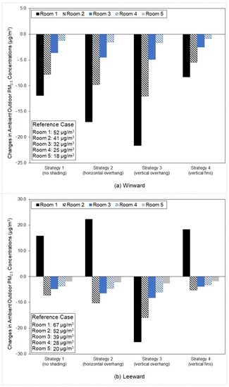
Figure 14.
The changes in ambient outdoor PM2.5 concentrations of individual rooms caused by exterior shading devices and heat rejection from outdoor units.
3.2.1. Windward Scenario
Results for Strategy 1 show that Rooms 1 to 4 experienced a reduction in ambient outdoor PM2.5 concentrations (Figure 14a). This reduction was largely attributable to the change in the pattern of the airflow within the street canyon. The counterclockwise vortex at the lower part of the street canyon carried fine particles from the street to the ambient outdoor environment of Rooms 1 to 4 (Figure 15a). When heat rejection was taken into account, the counterclockwise vortex moved closer to the surrounding building, in which case fine particles from the street were more easily carried by the vortex to the surrounding building (Figure 15b). There was no change in the ambient outdoor PM2.5 concentrations of Room 5, since fine particles from the street rarely traveled to Room 5 without winds blowing them upwards.
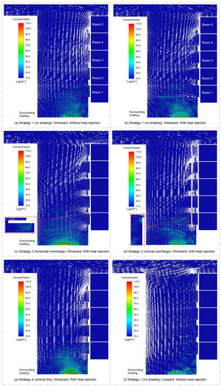

Figure 15.
The velocity vector and the contours of ambient outdoor PM2.5 concentrations for the building operating under different combinations of shading strategies and wind directions at 10:00.
Compared with Strategy 1, Strategy 2 predicted a greater reduction in the ambient outdoor PM2.5 concentrations of Rooms 1 to 4 (Figure 14a). This result was primarily because when horizontal overhangs were used, the counterclockwise vortex at the lower part of the street canyon moved closer to the surrounding building (Figure 15c). In addition, the movement of fine particles from the ambient outdoor environment of lower-floor rooms to the ambient outdoor environment of higher-floor rooms was partly blocked by horizontal overhangs. The reductions in the ambient outdoor PM2.5 concentrations of Rooms 1 to 4 predicted by Strategy 3 were also greater than those predicted by Strategy 1 (Figure 14a). This was likely due to the movement of fine particles from the street to the ambient outdoor environment of the building being partly blocked by vertical overhangs (Figure 15d). Rooms 1 to 4 experienced a smaller reduction in ambient outdoor PM2.5 concentrations under Strategy 4 than under Strategy 1 (Figure 14a). The comparison between the airflow pattern of Strategy 4 and that of Strategy 1 shows that the use of vertical fins led to a decrease in the speed of the winds within the street canyon (Figure 15b,e). A lower wind speed means that fine particles were harder to disperse, in which case the pollutant concentrations built up within the street canyon.
3.2.2. Leeward Scenario
Results for Strategy 1 indicate that Rooms 2 to 5 experienced a reduction in ambient outdoor PM2.5 concentrations while Room 1 experienced an increase in ambient outdoor PM2.5 concentrations (Figure 14b). In the absence of heat rejection, fine particles from the street were carried by upward winds to the ambient outdoor environment of the building (Figure 15f). In the presence of heat rejection, a clockwise vortex was produced above the outdoor unit of Room 1 (Figure 15g). This vortex was found to trap the fine particles from the street, resulting in the accumulation of fine particles within the ambient outdoor environment of Room 1. As a higher proportion of fine particles from the street were trapped within the ambient outdoor environment of Room 1, Rooms 2 to 5 experienced a reduction in ambient outdoor PM2.5 concentrations.
Compared with Strategy 1, Strategy 2 predicted a greater increase in the ambient outdoor PM2.5 concentrations of Room 1 and a greater reduction in the ambient outdoor PM2.5 concentrations of Rooms 2 to 5 (Figure 14b). One reason for this was the clockwise vortex produced above the outdoor unit of Room 1. Another reason was the horizontal overhang of Room 1, which prevented the fine particles from moving upwards and kept them contained within the ambient outdoor environment of Room 1 (Figure 15h). Strategy 3 predicted a reduction in the ambient outdoor PM2.5 concentrations of individual rooms, largely attributable to the blocking effect of vertical overhangs on the movement of fine particles from the street to the ambient outdoor environment of the building (Figure 15i). Strategy 4 predicted a greater increase in the ambient outdoor PM2.5 concentrations of Room 1 and a smaller reduction in the ambient outdoor PM2.5 concentrations of Rooms 2 to 5, compared to Strategy 1. This was related to a decrease in the speed of the winds within the street canyon caused using vertical fins, in which case a smaller number of fine particles were carried away from the street canyon (Figure 15g,j).
3.3. Cooling Loads
The changes in cooling loads due to exterior shading devices and heat rejection from outdoor units are shown in Figure 16, where the positive value means an increase in cooling loads compared to the reference case while the negative value means a decrease.
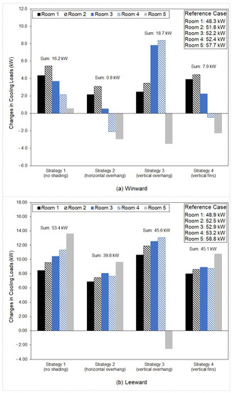
Figure 16.
The changes in cooling loads of individual rooms caused by exterior shading devices and heat rejection from outdoor units.
3.3.1. Windward Scenario
Under Strategy 1, the cooling loads of each room increased due to the increased ambient outdoor temperatures caused by heat rejection (described in Section 3.1.1). The results of Strategies 2, 3, and 4 show that for some rooms (including room 4 and Room 5 under Strategy 2, Room 5 under Strategy 3, and Room 4 and Room 5 under Strategy 4), the increase in cooling loads caused by heat rejection was more than offset using exterior shading devices. The change in the cooling loads of the building was calculated by adding up the changes in cooling loads of individual rooms. Under each strategy, the building had an increase in cooling loads, ranging from 0.8 kW to 18.7 kW. Comparisons between the four shading strategies show that Strategy 3 resulted in the highest increase in the cooling loads of the building, then Strategy 1, then Strategy 4, and finally Strategy 2. Surprisingly, the building had a greater increase in cooling loads after the implementation of vertical overhangs. This result indicates that in the presence of heat rejection, the use of vertical overhangs does not always mean lower demand for space cooling.
3.3.2. Leeward Scenario
Like the windward scenario, the leeward scenario predicted increased cooling loads for the building operating under Strategy 1. However, the increase in the cooling loads of the building was 69.7% smaller in the windward scenario than in the leeward scenario. The building had a lower increase in cooling loads after the implementation of exterior shading devices. Comparisons between the four strategies show that Strategy 1 resulted in the highest increase in the cooling loads of the building, then Strategy 3, then Strategy 4, and finally Strategy 2. When broken down by room, all the rooms had an increased demand for space cooling due to the increased ambient outdoor temperatures caused by heat rejection (described in Section 3.1.2), the exception being Room 5 under Strategy 3.
3.4. Indoor PM2.5 Exposure Concentrations
The changes in indoor PM2.5 exposure due to exterior shading devices and heat rejection from outdoor units were averaged over the occupied hours (09:00 to 18:00) are shown in Figure 17, where the positive value means an increase in exposure compared to the reference case while the negative value means a decrease.
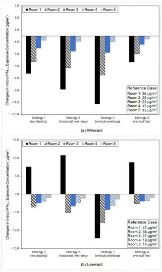
Figure 17.
The changes in indoor PM2.5 exposure concentrations of individual rooms caused by exterior shading devices and heat rejection from outdoor units.
3.4.1. Windward Scenario
The indoor PM2.5 exposure concentration of each room was positively correlated with the ambient outdoor PM2.5 concentrations described in Section 3.2.1. Results for Strategy 1 show a reduction in indoor PM2.5 exposure concentrations in Rooms 1 to 4, due to the reduced ambient outdoor PM2.5 concentrations. There was no change in indoor PM2.5 exposure concentrations of Room 5 since the ambient outdoor PM2.5 concentrations of Room 5 remained unchanged. Compared with Strategy 1, Strategies 2 and 3 predicted a greater reduction in indoor PM2.5 exposure concentrations in Rooms 1 to 4, while Strategy 4 predicted a smaller reduction. Comparisons between the four shading strategies show that Strategy 3 led to the greatest reduction in exposure, then Strategy 2, then Strategy 1, and finally Strategy 4.
3.4.2. Leeward Scenario
Like the windward scenario, the leeward scenario shows a positive correlation between indoor PM2.5 exposure concentrations and ambient outdoor PM2.5 concentrations. An increase in the indoor PM2.5 exposure concentrations of Room 1 could be seen under Strategies 1, 2, and 4, due to the increased ambient outdoor PM2.5 concentrations described in Section 3.2.2. A reduction in the indoor PM2.5 exposure concentrations of Rooms 2 to 5 could be seen under each strategy, attributable to the reduced ambient outdoor PM2.5 concentrations. Comparisons between the four shading strategies show that Strategy 3 led to the greatest reduction in the exposure of occupants to indoor PM2.5.
4. Discussion
4.1. Main Findings
This study has shown how a coupled simulation of EnergyPlus and Fluent can be used to understand the combined effects of exterior shading devices and heat rejection from outdoor units on the ambient outdoor temperatures, ambient outdoor PM2.5 concentrations, cooling loads, and indoor PM2.5 exposure concentrations of a building operating under different shading strategies.
The findings reported in this study suggest that heat rejection from outdoor units resulted in an increase in the ambient outdoor temperatures of the building and therefore caused an increase in cooling loads. The amount of the increase in cooling loads was found to vary in relation to the wind direction as well as the types of exterior shading devices. Averaged over the four shading strategies, the increase in the cooling loads of the building was 77.3% lower when outdoor units were on the windward side of the building (i.e., the windward scenario) than when outdoor units were on the leeward side (i.e., the leeward scenario). This finding may mean that for energy-saving purposes, the prevailing wind should be taken into consideration when placing outdoor units. As for the types of exterior shading devices, horizontal and vertical overhangs had a significant impact on the distribution of the heat from outdoor units while vertical fins had little impact. The use of horizontal overhangs helped reduce the accumulation of heat within the ambient outdoor environment of Rooms 1 to 4 and thus led to a lower increase in the ambient outdoor temperatures of these Rooms. In the windward scenario, the reduced accumulation of heat, in conjunction with the shading provided by horizontal overhangs, could almost offset the increase in the cooling loads of the building caused by heat rejection. The use of vertical overhangs was found to increase the accumulation of heat within the ambient outdoor environment of certain rooms (including Room 3 and Room 4 in the windward scenario and Rooms 1 to 4 in the leeward scenario) and caused a greater increase in the ambient outdoor temperatures of these rooms. In both windward and leeward scenarios, the increase in the cooling loads of the building was greater when vertical overhangs were used than when horizontal overhangs were used. Therefore, when heat rejection is taken into account, horizontal overhangs are considered to be a better energy-efficiency strategy than vertical overhangs.
In the windward scenario, occupants of Rooms 1 to 4 faced a reduced risk of exposure to indoor PM2.5 because of the reduction in ambient outdoor PM2.5 concentrations caused by heat rejection, while those of Room 5 saw no change in indoor PM2.5 exposure. In the leeward scenario, occupants of Room 1 might face an increased risk of exposure to indoor PM2.5 since heat rejection could cause an increase in the ambient outdoor PM2.5 concentrations of Room 1. These findings, in conjunction with the one that the increase in cooling loads caused by heat rejection was smaller in the windward scenario than in the leeward scenario, may mean that placing outdoor units on the windward side of the building rather than on the leeward side can help achieve better energy efficiency and improved occupant health. The airflow pattern within the street canyon played a key role in the transport of fine particles from the street. Both horizontal and vertical overhangs were found to have a blocking effect on the movement of fine particles from the street to the ambient outdoor environment of the building. The horizontal overhangs could also lead to the counterclockwise vortex at the bottom of the street canyon being moved closer to the surrounding building, in which case fine particles from the street were more easily carried by winds to the surrounding building. The speed of winds within the street canyon decreased when vertical fins were used. A reduced wind speed means that PM2.5 concentrations can build up within the street canyon, therefore causing higher indoor PM2.5 exposure. Therefore, outdoor units should be coupled with overhangs rather than vertical fins to improve indoor air quality.
4.2. Limitations and Future Research
The models developed in this study have several limitations. The exterior shading devices were modeled in a fixed position. However, variations in the position of exterior shading devices, such as the distance between vertical overhangs and the exterior surfaces of the building or the distance between two vertical fins, can significantly influence model outcomes. In terms of the position of outdoor units, in addition to the modeled arrangement (i.e., outdoor units being placed right below windows), there are several other common ways of placing outdoor units (e.g., next to windows, above windows, or in front of windows). Further research on buildings with different arrangements of exterior shading devices or outdoor units is therefore worth investigating. Additionally, scenarios where some of the outdoor units of the building were not switched on were worth investigating in future studies. Some modeling studies [59,60,61] support the conclusion that the aspect ratio acts as an important modifier of the pattern of the airflow within a street canyon. Therefore, the effect of heat rejection from outdoor units on the pattern of the airflow within a street canyon can also vary depending on the aspect ratio. In addition, a large aspect ratio can reduce the shading effect of exterior shading devices, and vice versa [62]. Further work will be needed to explore the sensitivity of the model to different aspect ratios. The penetration factor and deposition rate of PM2.5 are largely dependent on particle size [42]. For simplicity, a single penetration factor and a single deposition rate were applied, under the assumption that the particles modeled in this study had the same size. Indoor sources (e.g., cooking and smoking) are an important modifier of indoor PM2.5 exposure, but have not been considered in this study. Indoor- and outdoor-sourced PM2.5 with different sizes will be modeled in future research. A low-rise building was modeled in this study to reduce computational costs, while it is acknowledged that the modeled building height cannot represent the bulk of building heights seen in the Hong Kong building stock. The sensitivity of the model to variations in building height will be explored in future research.
In some cases, the research findings may not apply to buildings that have the same built form, the same arrangement of outdoor units, and the same arrangement of exterior shading devices as the modeled building. Cooling was modeled to a 25 °C set-point, while certain people may prefer a higher indoor temperature. An increased cooling set-point can lead to a reduction in the use of air conditioning. The reduced use of air conditioning can decrease the amount of heat rejected by outdoor units, therefore reducing the effect of heat rejection on the ambient outdoor environment. Similarly, a lower cooling set-point means a greater amount of heat rejected by outdoor units, in which case the effect of heat rejection on the ambient outdoor environment can be magnified. Buildings with a different orientation (e.g., an east-west orientation) are expected to obtain different amounts of heat from the sun, leading to a change in cooling loads. The amount of heat rejected by outdoor units can vary significantly based on cooling loads. Building airtightness was applied using a permeability of 11.5 m3/h/m2, while some buildings such as those being recently built may have lower rates of infiltration of outdoor air. Buildings with a lower permeability are predicted to have lower levels of pollution from outdoor sources. As in previous studies [19,21,44,60,61], symmetry-boundary conditions were applied to non-inlet/outlet laterals and sky to reduce the extent of the computational model to a symmetric subsection of the overall physical system. There was zero flux of heat across the symmetry boundary. However, it is acknowledged that this simplified boundary condition could lead to an overestimation of the accumulation of heat within the street canyon. Although the literature-based validation carried out in Section 2.3.1 and Section 2.3.2 has shown that the airflow and pollution models developed in this study could give accurate estimates of airflow patterns around buildings and outdoor air pollutant concentrations, the boundary conditions used in the validation did not reflect the actual ones seen in the Hong Kong building stock. Validation based on the actual buildings in Hong Kong should be conducted to further check model accuracy.
5. Conclusions
This paper reports the results of coupled EnergyPlus-Fluent simulations, illustrating the combined effects of exterior shading devices (including horizontal overhangs, vertical overhangs, and vertical fins) and heat rejection from outdoor units on the ambient outdoor environment of a six-story building and how changes in the ambient outdoor environment could affect cooling loads and indoor PM2.5 exposure. The main outcomes of this paper are:
- In the windward scenario (i.e., outdoor units on the windward side of the building), some of the heat from outdoor units was discharged to the middle of the street canyon. In the leeward scenario (i.e., outdoor units on the leeward side of the building), the heat from outdoor units was contained in the ambient outdoor environment of the building. The increase in ambient outdoor temperatures caused by heat rejection was on average 1.4 °C higher in the leeward scenario than in the windward scenario;
- The increased ambient outdoor temperatures caused by heat rejection increased the cooling loads of the building, ranging from 0.8 kW in the windward scenario with the use of horizontal overhangs to 53.4 kW in the leeward scenario with no shading devices. In the windward scenario, the ability of horizontal overhangs to reduce solar heat gains and reduce the accumulation of heat within the ambient outdoor environment of the building could almost offset the increase in cooling loads caused by heat rejection. The use of vertical overhangs, on the other hand, does not always mean lower demand for space cooling. When heat rejection was taken into account, horizontal overhangs were considered to be a better energy-efficiency strategy than vertical overhangs;
- In the windward scenario, heat rejection from outdoor units, horizontal overhangs, and vertical overhangs helped limit the movement of PM2.5 from the street to the ambient outdoor environment of the building; occupants thus had a reduced risk of exposure to indoor PM2.5. In the leeward scenario, heat rejection from outdoor units, horizontal overhangs, and vertical fins were found to increase the accumulation of PM2.5 within the ambient environment of the bottom-floor room; occupants of this room thus faced an increased risk of exposure to indoor PM2.5. Outdoor units should be coupled with overhangs rather than vertical fins to improve indoor air quality;
- The combination of outcomes (1), (2), and (3) means that to achieve better energy efficiency and improved occupant health, outdoor units should be coupled with horizontal overhangs and need to be placed on the windward side of the building rather than on the leeward side.
Author Contributions
Conceptualization, X.Z., Z.Z. and R.Z.; methodology, X.Z. and Z.Z.; software, Z.Z.; validation, X.Z., Z.Z. and R.Z.; formal analysis, X.Z. and Z.Z.; investigation, X.Z., Z.Z. and Z.W.; resources, Z.Z. and Z.W.; data curation, Z.Z.; writing—original draft preparation, X.Z. and Z.Z.; writing—review and editing, X.Z., Z.Z., R.Z. and Z.W.; visualization, X.Z. and Z.Z.; supervision, Z.Z. and Z.W.; project administration, Z.Z. and Z.W.; funding acquisition, X.Z. and Z.Z. All authors have read and agreed to the published version of the manuscript.
Funding
This research was supported by Zhejiang Provincial Natural Science Foundation of China under Grant No. LQ22E080026 and Major Science and Technology Program of Ningbo Science and Technology Bureau under Project Code 2022Z161.
Data Availability Statement
The data presented in this study are available on request from the corresponding author.
Acknowledgments
The authors would like to thank the Department of Architecture and Built Environment, University of Nottingham Ningbo China, and the School of Energy and Environment, City University of Hong Kong, for providing materials used for experiments and simulations.
Conflicts of Interest
The authors declare no conflict of interest.
References
- EMSD. Building Energy Codes; Electrical and Mechanical Services Department: Hong Kong, China, 2020.
- EMSD. Hong Kong Energy End-Use Data 2022; Electrical and Mechanical Services Department: Hong Kong, China, 2022.
- Lauzet, N.; Rodler, A.; Musy, M.; Azam, M.-H.; Guernouti, S.; Mauree, D.; Colinart, T. How building energy models take the local climate into account in an urban context—A review. Renew. Sustain. Energy Rev. 2019, 116, 109390. [Google Scholar] [CrossRef]
- Nada, S.; Said, M. Performance and energy consumptions of split type air conditioning units for different arrangements of outdoor units in confined building shafts. Appl. Therm. Eng. 2017, 123, 874–890. [Google Scholar] [CrossRef]
- Nada, S.; Said, M. Solutions of thermal performance problems of installing AC outdoor units in buildings light wells using mechanical ventilations. Appl. Therm. Eng. 2018, 131, 295–310. [Google Scholar] [CrossRef]
- Kim, G.; Lim, H.S.; Lim, T.S.; Schaefer, L.; Kim, J.T. Comparative advantage of an exterior shading device in thermal performance for residential buildings. Energy Build. 2012, 46, 105–111. [Google Scholar] [CrossRef]
- Rabani, M.; Madessa, H.B.; Nord, N. Achieving zero-energy building performance with thermal and visual comfort enhancement through optimization of fenestration, envelope, shading device, and energy supply system. Sustain. Energy Technol. Assess. 2021, 44, 101020. [Google Scholar] [CrossRef]
- Chow, T.; Lin, Z. Prediction of on-coil temperature of condensers installed at tall building re-entrant. Appl. Therm. Eng. 1999, 19, 117–132. [Google Scholar] [CrossRef]
- Hsieh, C.-M.; Aramaki, T.; Hanaki, K. Managing heat rejected from air conditioning systems to save energy and improve the microclimates of residential buildings. Comput. Environ. Urban Syst. 2011, 35, 358–367. [Google Scholar] [CrossRef]
- Han, M.; Chen, H. Effect of external air-conditioner units’ heat release modes and positions on energy consumption in large public buildings. Build. Environ. 2017, 111, 47–60. [Google Scholar] [CrossRef]
- Cui, D.; Li, X.; Liu, J.; Yuan, L.; Mak, C.M.; Fan, Y.; Kwok, K. Effects of building layouts and envelope features on wind flow and pollutant exposure in height-asymmetric street canyons. Build. Environ. 2021, 205, 108177. [Google Scholar] [CrossRef]
- Xiong, Y.; Chen, H. Effects of sunshields on vehicular pollutant dispersion and indoor air quality: Comparison between isothermal and nonisothermal conditions. Build. Environ. 2021, 197, 107854. [Google Scholar] [CrossRef]
- Zheng, J.; Tao, Q.; Chen, Y. Airborne infection risk of inter-unit dispersion through semi-shaded openings: A case study of a multi-storey building with external louvers. Build. Environ. 2022, 225, 109586. [Google Scholar] [CrossRef] [PubMed]
- Adelia, A.; Yuan, C.; Liu, L.; Shan, R. Effects of urban morphology on anthropogenic heat dispersion in tropical high-density residential areas. Energy Build. 2019, 186, 368–383. [Google Scholar] [CrossRef]
- Cohen, A.J.; Anderson, H.R.; Ostro, B.; Pandey, K.D.; Krzyzanowski, M.; Künzli, N.; Gutschmidt, K.; Pope, A.; Romieu, I.; Samet, J.M.; et al. The Global Burden of Disease Due to Outdoor Air Pollution. J. Toxicol. Environ. Health Part A 2005, 68, 1301–1307. [Google Scholar] [CrossRef] [PubMed]
- Keshavarzian, E.; Kwok, K.C.; Dong, K.; Chauhan, K.; Zhang, Y. An experimental Investigation of stagnant air pollution dispersion around a building in a turbulent flow. Build. Environ. 2022, 224, 109564. [Google Scholar] [CrossRef]
- Ng, W.-Y.; Chau, C.-K. A modeling investigation of the impact of street and building configurations on personal air pollutant exposure in isolated deep urban canyons. Sci. Total Environ. 2014, 468–469, 429–448. [Google Scholar] [CrossRef]
- Meng, M.-R.; Cao, S.-J.; Kumar, P.; Tang, X.; Feng, Z. Spatial distribution characteristics of PM2.5 concentration around residential buildings in urban traffic-intensive areas: From the perspectives of health and safety. Saf. Sci. 2021, 141, 105318. [Google Scholar] [CrossRef]
- Wen, Y.-B.; Huang, Z.-R.; Tang, Y.-F.; Li, D.-R.; Zhang, Y.-J.; Zhao, F.-Y. Air exchange rate and pollutant dispersion inside compact urban street canyons with combined wind and thermal driven natural ventilations: Effects of non-uniform building heights and unstable thermal stratifications. Sci. Total Environ. 2022, 851, 158053. [Google Scholar] [CrossRef]
- Jones, N.; Thornton, C.; Mark, D.; Harrison, R. Indoor/outdoor relationships of particulate matter in domestic homes with roadside, urban and rural locations. Atmos. Environ. 2000, 34, 2603–2612. [Google Scholar] [CrossRef]
- Canha, N.; Almeida, S.M.; Freitas, M.D.C.; Trancoso, M.; Sousa, A.; Mouro, F.; Wolterbeek, H.T. Particulate matter analysis in indoor environments of urban and rural primary schools using passive sampling methodology. Atmos. Environ. 2014, 83, 21–34. [Google Scholar] [CrossRef]
- Semmens, E.O.; Noonan, C.W.; Allen, R.W.; Weiler, E.C.; Ward, T.J. Indoor particulate matter in rural, wood stove heated homes. Environ. Res. 2015, 138, 93–100. [Google Scholar] [CrossRef]
- Taylor, J.; Davies, M.; Mavrogianni, A.; Shrubsole, C.; Hamilton, I.; Das, P.; Jones, B.; Oikonomou, E.; Biddulph, P. Mapping indoor overheating and air pollution risk modification across Great Britain: A modelling study. Build. Environ. 2016, 99, 1–12. [Google Scholar] [CrossRef]
- Taylor, J.; Shrubsole, C.; Symonds, P.; Mackenzie, I.; Davies, M. Application of an indoor air pollution metamodel to a spatially-distributed housing stock. Sci. Total Environ. 2019, 667, 390–399. [Google Scholar] [CrossRef] [PubMed]
- Taylor, J.; Shrubsole, C.; Davies, M.; Biddulph, P.; Das, P.; Hamilton, I.; Vardoulakis, S.; Mavrogianni, A.; Jones, B.; Oikonomou, E. The modifying effect of the building envelope on population exposure to PM2.5 from outdoor sources. Indoor Air 2014, 24, 639–651. [Google Scholar] [CrossRef] [PubMed]
- Crawley, D.B.; Lawrie, L.K.; Winkelmann, F.C.; Buhl, W.; Huang, Y.; Pedersen, C.O.; Strand, R.K.; Liesen, R.J.; Fisher, D.E.; Witte, M.J.; et al. EnergyPlus: Creating a new-generation building energy simulation program. Energy Build. 2001, 33, 319–331. [Google Scholar] [CrossRef]
- Ansys Fluids: Computational Fluid Dynamics (CFD) Simulation Software, Version 2021; Ansys, Inc.: Canonsburg, PA, USA, 2021.
- HKO. Climatological Information Services. 2021. Available online: https://www.hko.gov.hk/en/cis/climat.htm (accessed on 1 June 2023).
- Environmental Protection Interactive Centre: Air Quality Data—Download/Display 2021. Available online: https://cd.epic.epd.gov.hk/EPICDI/air/station/?lang=en (accessed on 24 May 2023).
- Wan, K.; Yik, F. Representative building design and internal load patterns for modelling energy use in residential buildings in Hong Kong. Appl. Energy 2004, 77, 69–85. [Google Scholar] [CrossRef]
- BEAM Plus New Buildings, Version 2.0; BEAM Society: Hong Kong, China, 2019.
- Buildings Department Hong Kong. Guidelines on Design and Construction Requirements for Energy Efficiency of Residential Buildings; Buildings Department Hong Kong: Hong Kong, China, 2014. [Google Scholar]
- Bojic, M.; Yik, F.; Leung, W. Thermal insulation of cooled spaces in high rise residential buildings in Hong Kong. Energy Convers. Manag. 2002, 43, 165–183. [Google Scholar] [CrossRef]
- ISO 13790; Energy Performance of Buildings, Calculation of Energy Use for Space Heating and Cooling. International Organization for Standardization: Geneva, Switzerland, 2008.
- CIBSE. CIBSE Guide A: Environmental Design; The Chartered Institution of Building Services Engineers: London, UK, 2006. [Google Scholar]
- Daikin. Engineering Data; Daikin AC: New York, NY, USA, 2022. [Google Scholar]
- Kikegawa, Y.; Genchi, Y.; Yoshikado, H.; Kondo, H. Development of a numerical simulation system toward comprehensive assessments of urban warming countermeasures including their impacts upon the urban buildings’ energy-demands. Appl. Energy 2003, 76, 449–466. [Google Scholar] [CrossRef]
- Yu, F.; Ho, W. Tactics for carbon neutral office buildings in Hong Kong. J. Clean. Prod. 2021, 326, 129369. [Google Scholar] [CrossRef]
- Alonso, M.J.; Dols, W.; Mathisen, H. Using Co-simulation between EnergyPlus and CONTAM to evaluate recirculation-based, demand-controlled ventilation strategies in an office building. Build. Environ. 2022, 211, 108737. [Google Scholar] [CrossRef]
- Jones, B.; Das, P.; Chalabi, Z.; Davies, M.; Hamilton, I.; Lowe, R.; Milner, J.; Ridley, I.; Shrubsole, C.; Wilkinson, P. The Effect of Party Wall Permeability on Estimations of Infiltration from Air Leakage. Int. J. Vent. 2013, 12, 17–30. [Google Scholar] [CrossRef]
- Taylor, J.; Mavrogianni, A.; Davies, M.; Das, P.; Shrubsole, C.; Biddulph, P.; Oikonomou, E. Understanding and mitigating overheating and indoor PM2.5 risks using coupled temperature and indoor air quality models. Build. Serv. Eng. Res. Technol. 2015, 36, 275–289. [Google Scholar] [CrossRef]
- Long, C.M.; Suh, H.H.; Catalano, P.J.; Koutrakis, P. Using Time- and Size-Resolved Particulate Data to Quantify Indoor Penetration and Deposition Behavior. Environ. Sci. Technol. 2001, 35, 2089–2099. [Google Scholar] [CrossRef] [PubMed]
- Liu, J.; Heidarinejad, M.; Pitchurov, G.; Zhang, L.; Srebric, J. An extensive comparison of modified zero-equation, standard k-ε, and LES models in predicting urban airflow. Sustain. Cities Soc. 2018, 40, 28–43. [Google Scholar] [CrossRef]
- Zhang, R.; Mirzaei, P.A.; Jones, B. Development of a dynamic external CFD and BES coupling framework for application of urban neighbourhoods energy modelling. Build. Environ. 2018, 146, 37–49. [Google Scholar] [CrossRef]
- Chu, C.-R.; Yang, K.-J. Transport process of outdoor particulate matter into naturally ventilated buildings. Build. Environ. 2022, 207, 108424. [Google Scholar] [CrossRef]
- Franke, J.; Hellsten, A.; Schluenzen, K.H.; Carissimo, B. The COST 732 Best Practice Guideline for CFD simulation of flows in the urban environment: A summary. Int. J. Environ. Pollut. 2011, 44, 419–427. [Google Scholar] [CrossRef]
- Tominaga, Y.; Mochida, A.; Yoshie, R.; Kataoka, H.; Nozu, T.; Yoshikawa, M.; Shirasawa, T. AIJ guidelines for practical applications of CFD to pedestrian wind environment around buildings. J. Wind Eng. Ind. Aerodyn. 2008, 96, 1749–1761. [Google Scholar] [CrossRef]
- Snyder, W. Guideline for Fluid Modeling of Atmospheric Diffusion. In Fluid Modeling; Report No. 10; U.S. Environmental Protection Agency: Washington, DC, USA, 1981. [Google Scholar]
- Roache, P.J. Perspective: A Method for Uniform Reporting of Grid Refinement Studies. J. Fluids Eng. 1994, 116, 405–413. [Google Scholar] [CrossRef]
- Keshavarzian, E.; Jin, R.; Dong, K.; Kwok, K.C. Effect of building cross-section shape on air pollutant dispersion around buildings. Build. Environ. 2021, 197, 107861. [Google Scholar] [CrossRef]
- Shirzadi, M.; Tominaga, Y. CFD evaluation of mean and turbulent wind characteristics around a high-rise building affected by its surroundings. Build. Environ. 2022, 225, 109637. [Google Scholar] [CrossRef]
- Gdeisat; Lilley, F. 1—MATLAB® Integrated Development Environment. In Matlab by Example; Gdeisat, M., Lilley, F., Eds.; Elsevier: Oxford, UK, 2013; pp. 1–20. [Google Scholar]
- Dai, T.; Liu, S.; Liu, J.; Jiang, N.; Liu, W.; Chen, Q. Evaluation of fast fluid dynamics with different turbulence models for predicting outdoor airflow and pollutant dispersion. Sustain. Cities Soc. 2022, 77, 103583. [Google Scholar] [CrossRef]
- Tominaga, Y.; Stathopoulos, T. CFD simulations of near-field pollutant dispersion with different plume buoyancies. J. Affect. Disord. 2018, 131, 128–139. [Google Scholar] [CrossRef]
- Hanna, S.; Chang, J. Acceptance criteria for urban dispersion model evaluation. Meteorol. Atmos. Phys. 2012, 116, 133–146. [Google Scholar] [CrossRef]
- Chen, G.; Rong, L.; Zhang, G. Impacts of urban geometry on outdoor ventilation within idealized building arrays under unsteady diurnal cycles in summer. Build. Environ. 2021, 206, 108344. [Google Scholar] [CrossRef]
- Leitl, B.; Schatzmann, M.C. Compilation of Experimental Data for Validation of Microscale Dispersion Models; Meteorological Institute of the University of Hamburg: Hamburg, Germany, 2010. [Google Scholar]
- ASHRAE. Guideline 14–2014: Measurement of Energy, Demand, and Water Savings; American Society of Heating, Refrigeratng, and Air Conditioning Engineers: Atlanta, GA, USA, 2014. [Google Scholar]
- Liu, D.; Shi, Y. The Influence Mechanism of Urban Spatial Structure on Urban Vitality Based on Geographic Big Data: A Case Study in Downtown Shanghai. Buildings 2022, 12, 569. [Google Scholar] [CrossRef]
- Hang, J.; Liang, J.; Wang, X.; Zhang, X.; Wu, L.; Shao, M. Investigation of O3–NOx–VOCs chemistry and pollutant dispersion in street canyons with various aspect ratios by CFD simulations. Build. Environ. 2022, 226, 109667. [Google Scholar] [CrossRef]
- Ghobadi, P.; Nasrollahi, N. Assessment of pollutant dispersion in deep street canyons under different source positions: Numerical simulation. Urban Clim. 2021, 40, 101027. [Google Scholar] [CrossRef]
- Albatayneh, A. Optimising the Parameters of a Building Envelope in the East Mediterranean Saharan, Cool Climate Zone. Buildings 2021, 11, 43. [Google Scholar] [CrossRef]
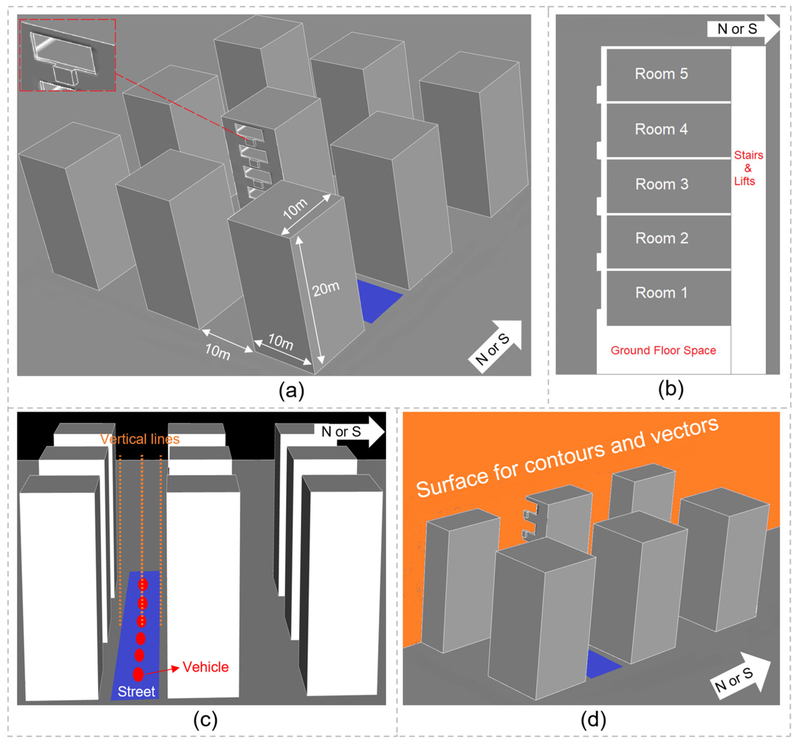
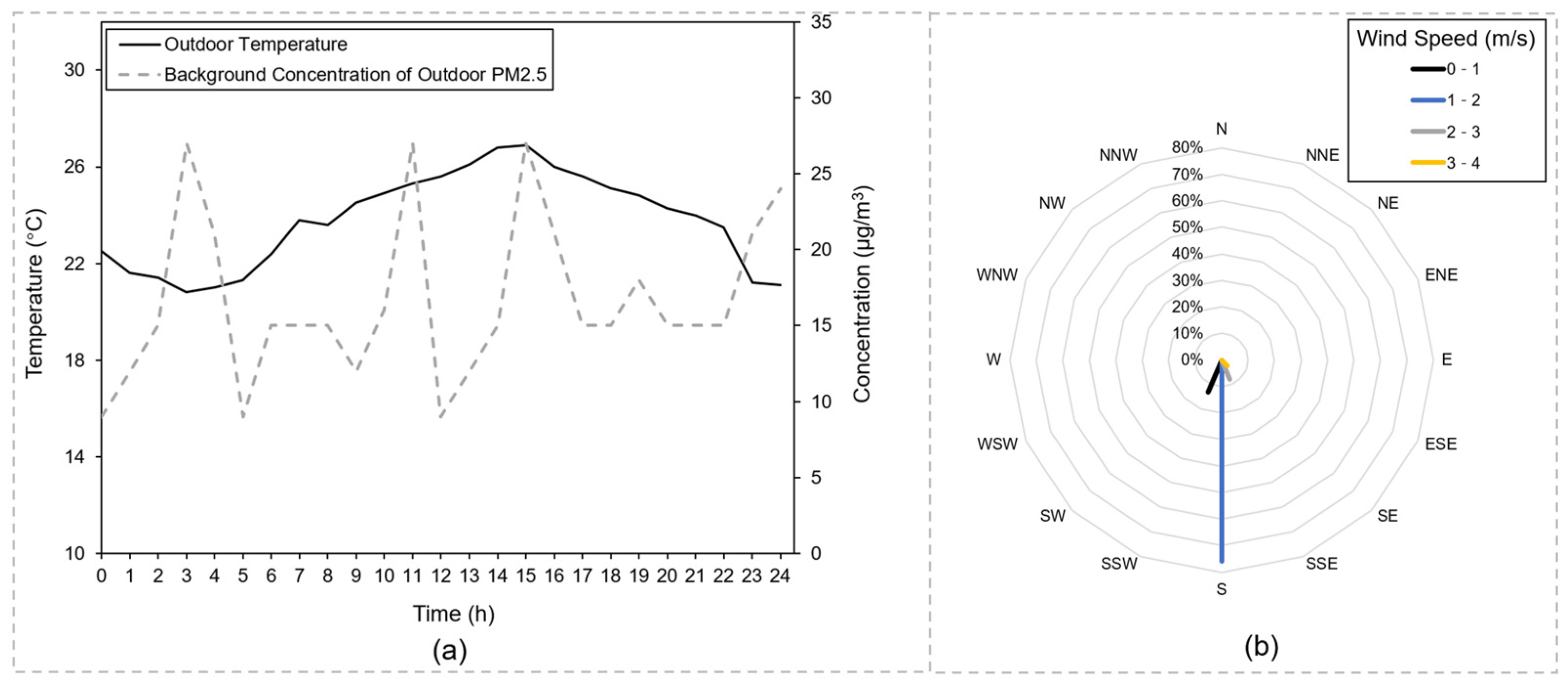

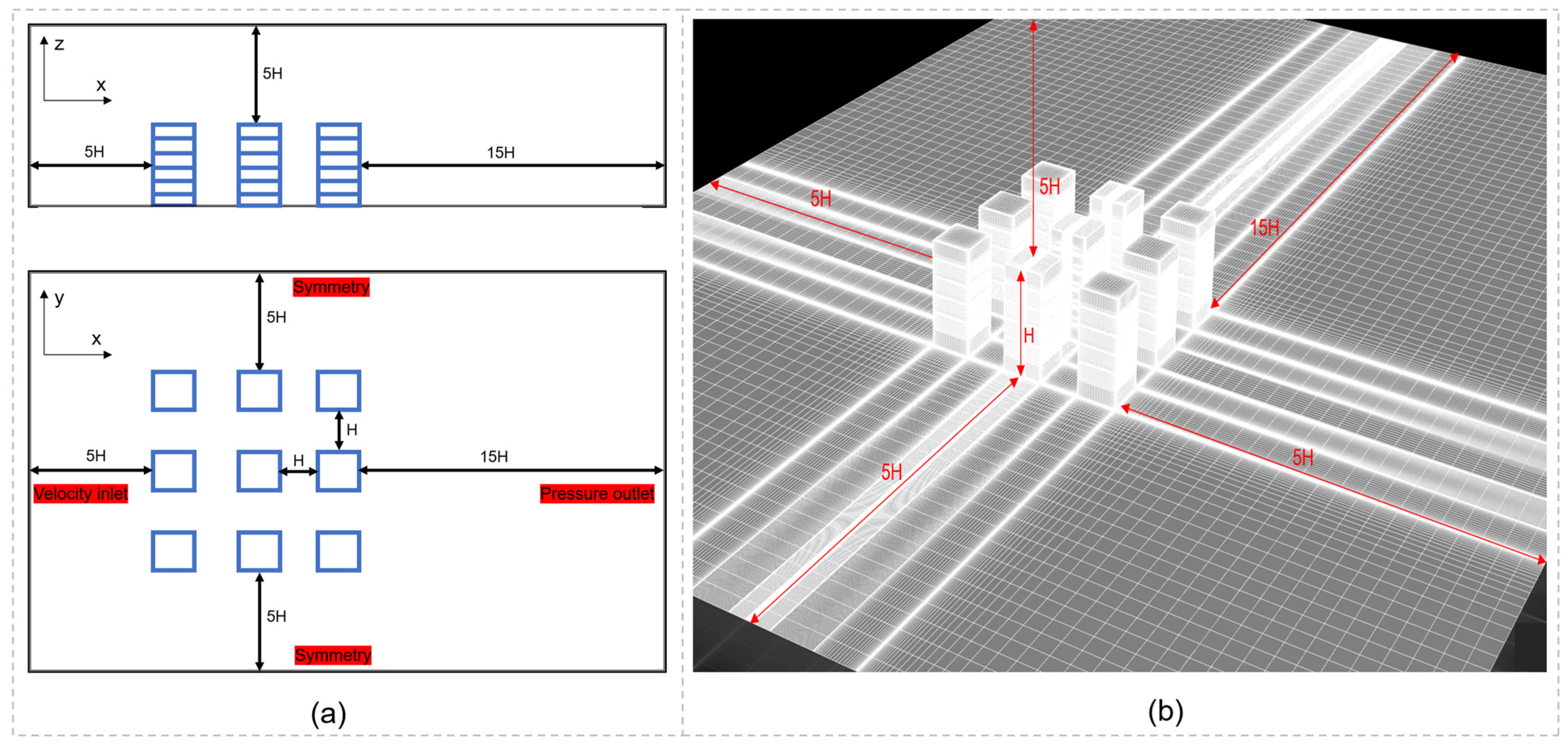
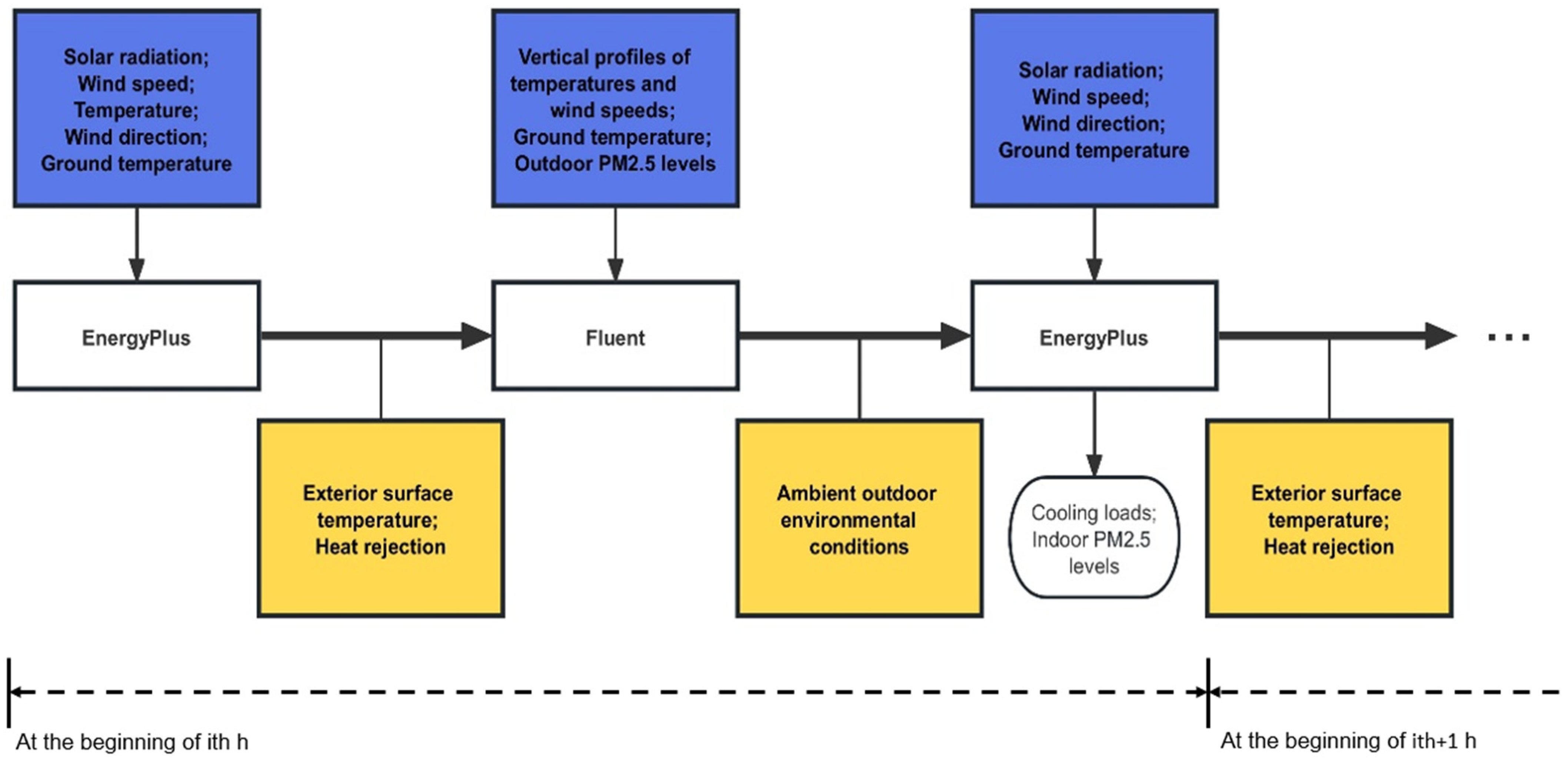
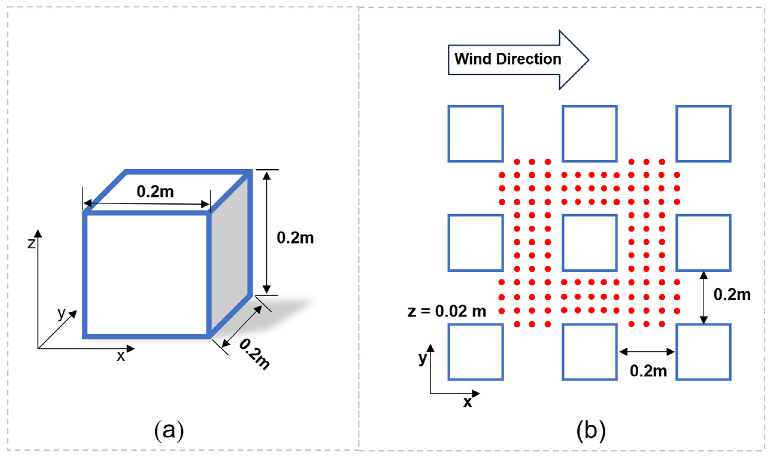

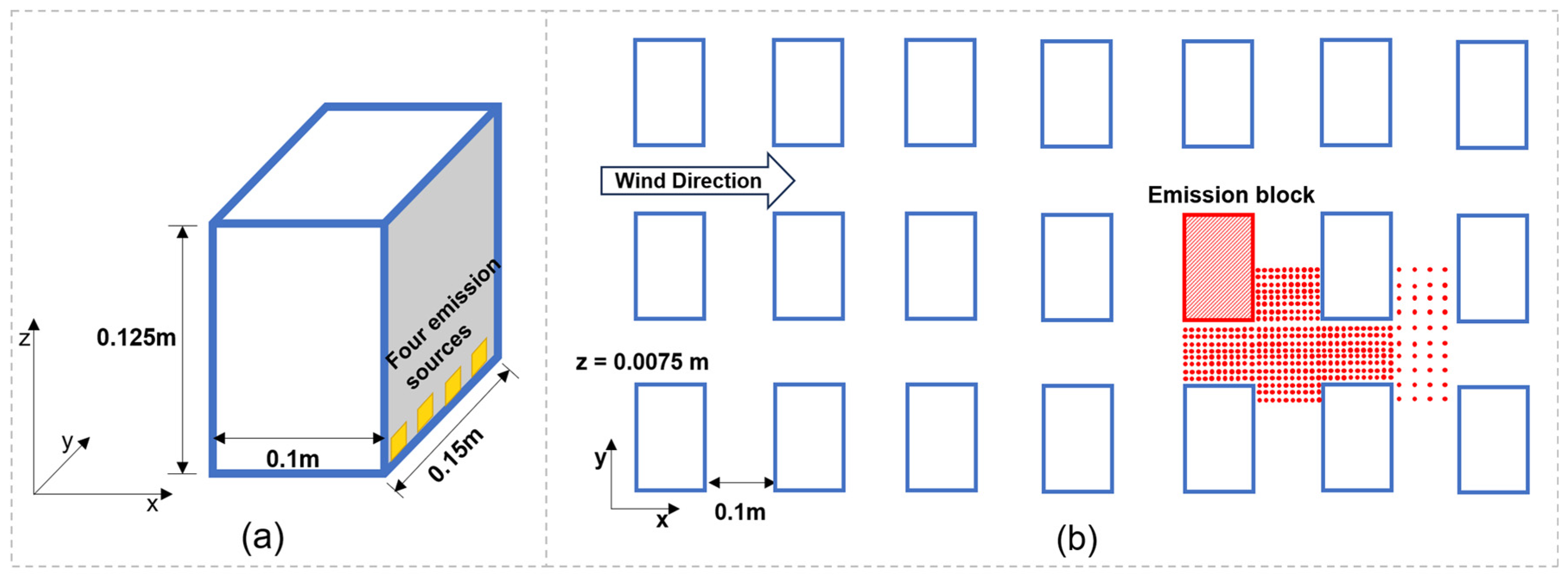
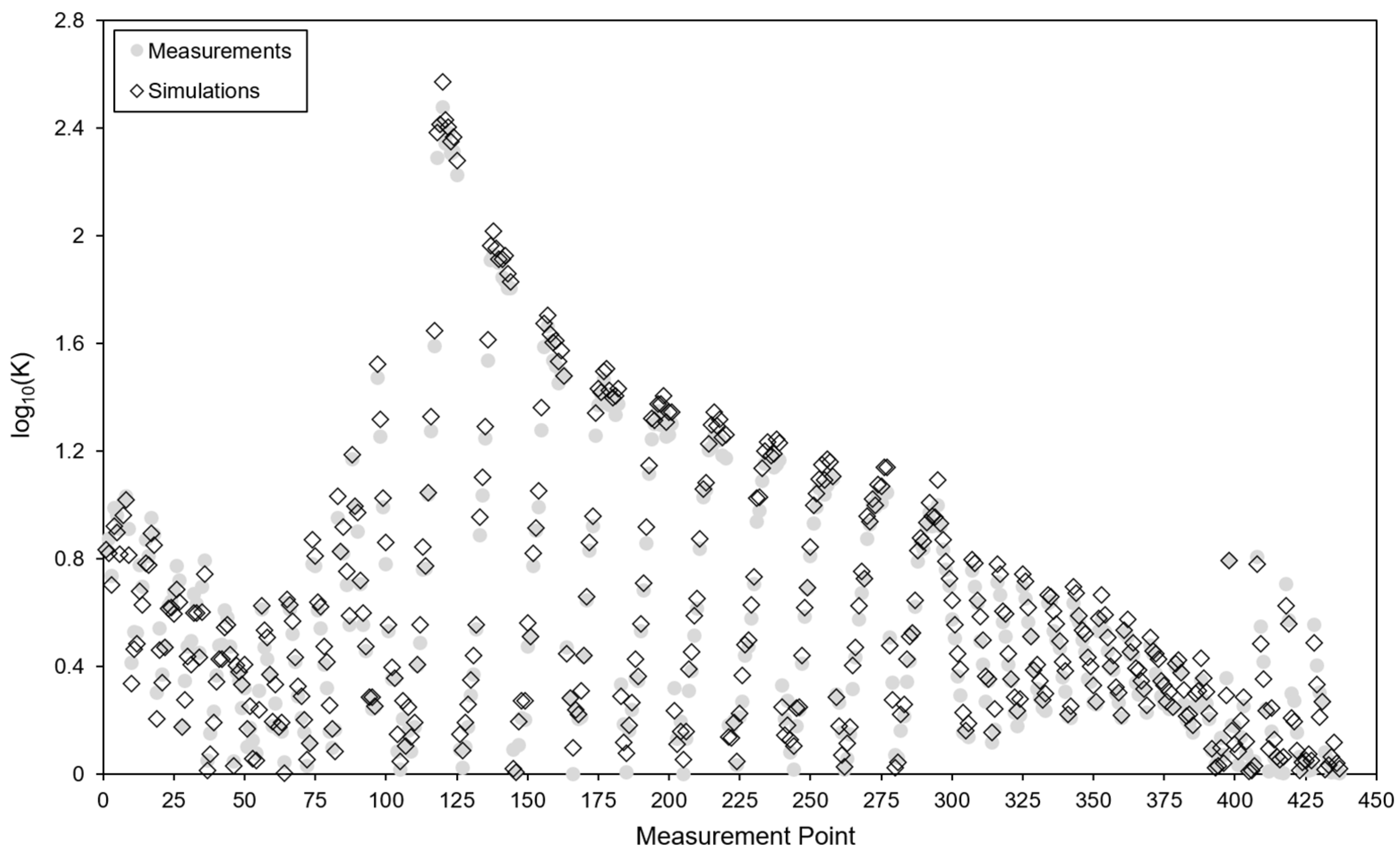

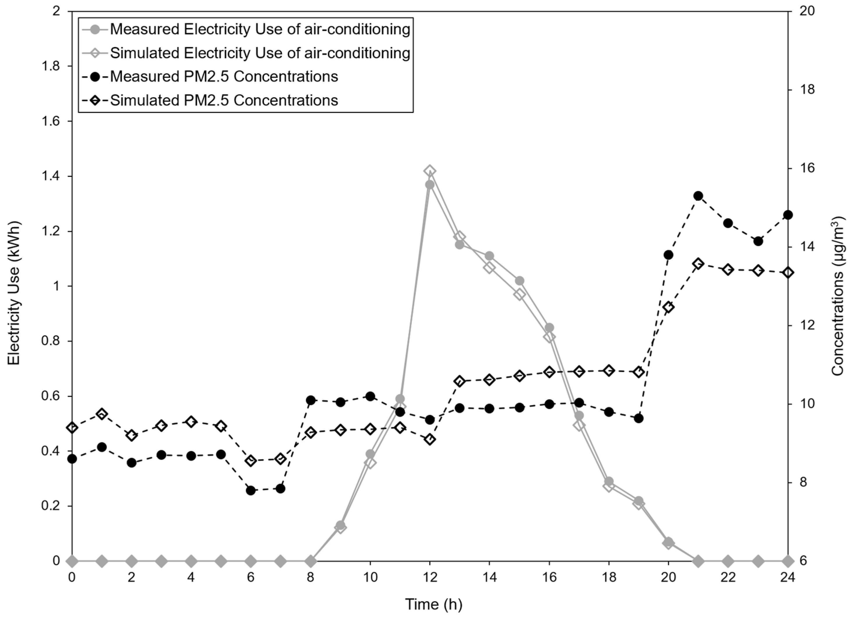
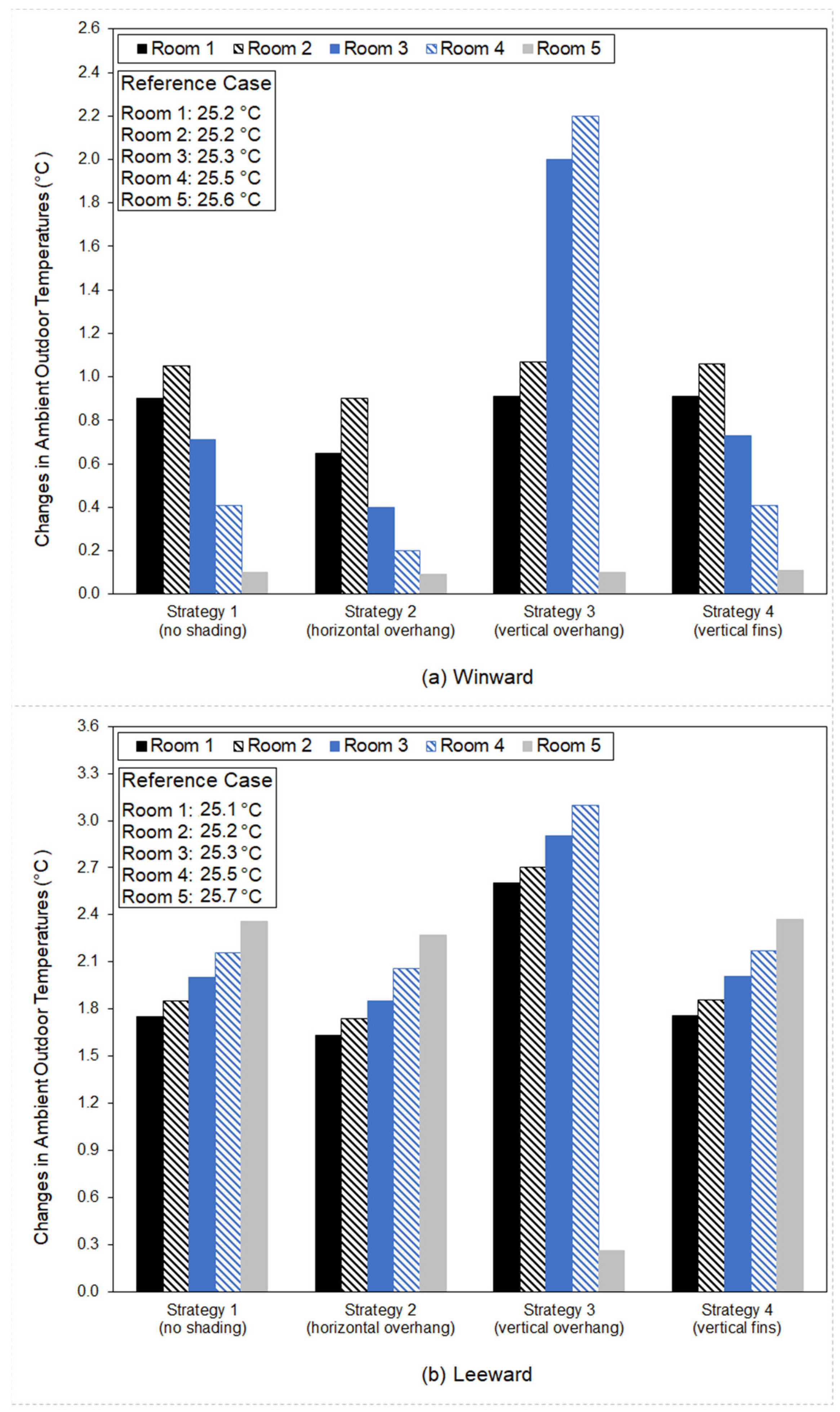


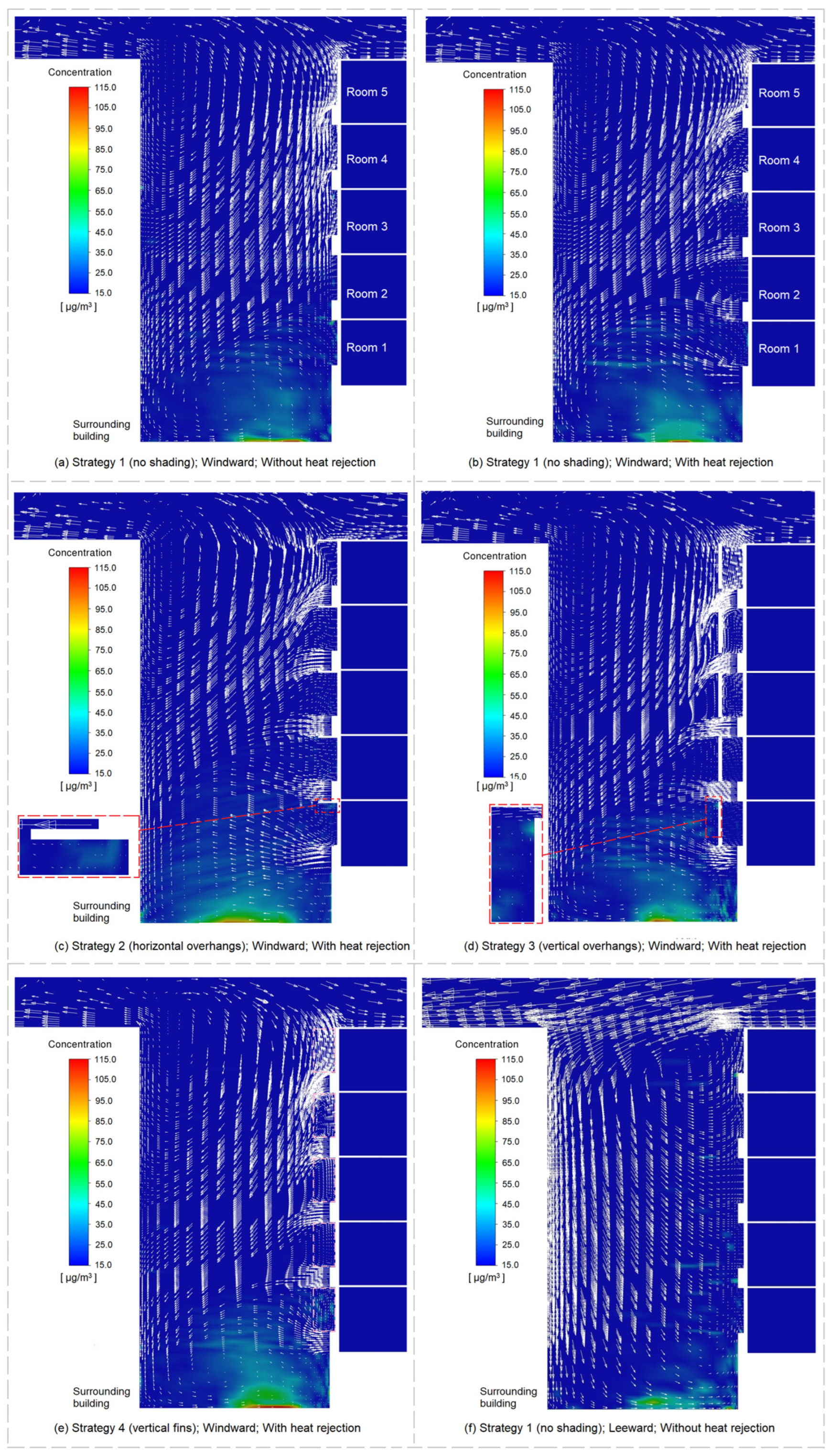
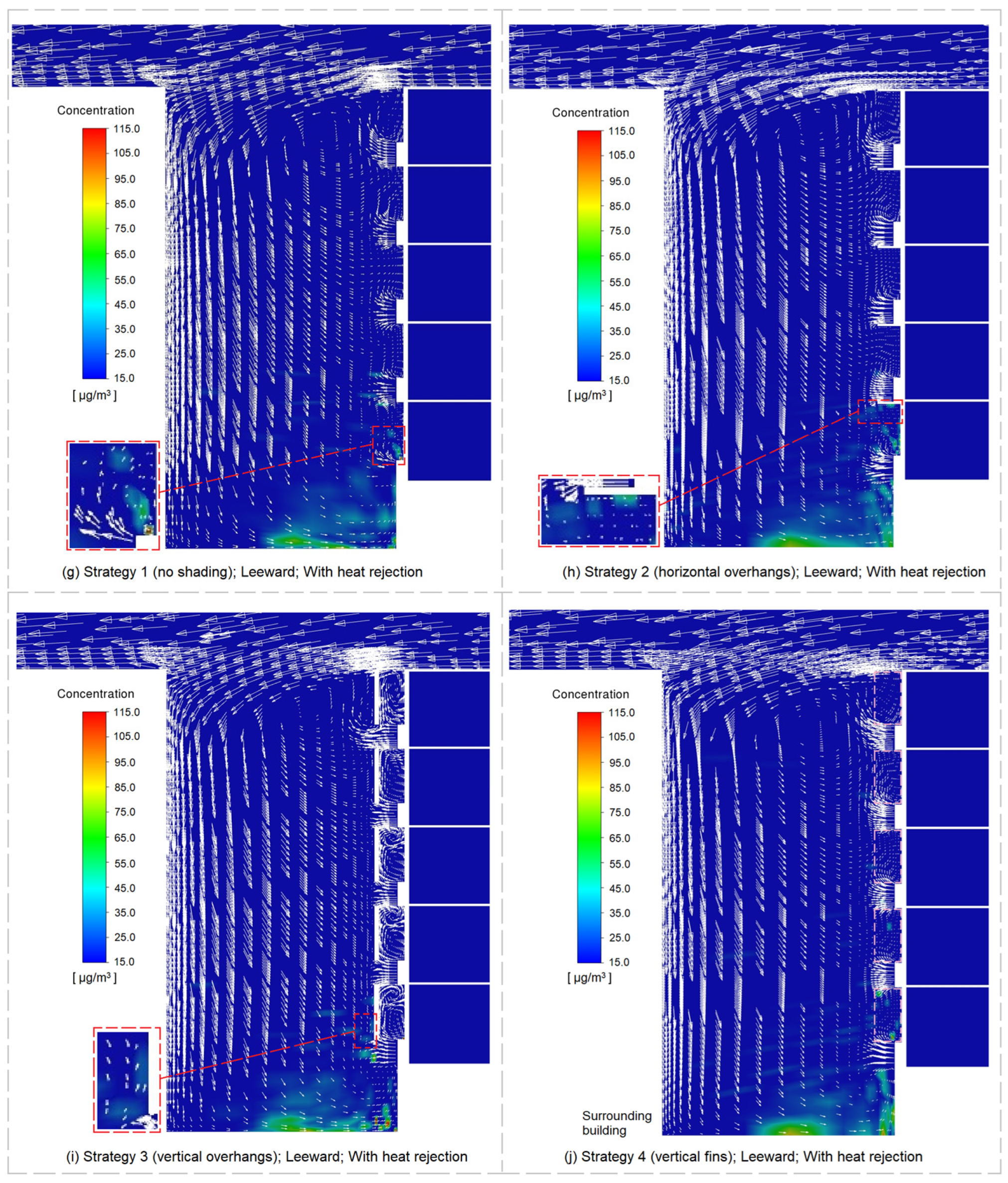
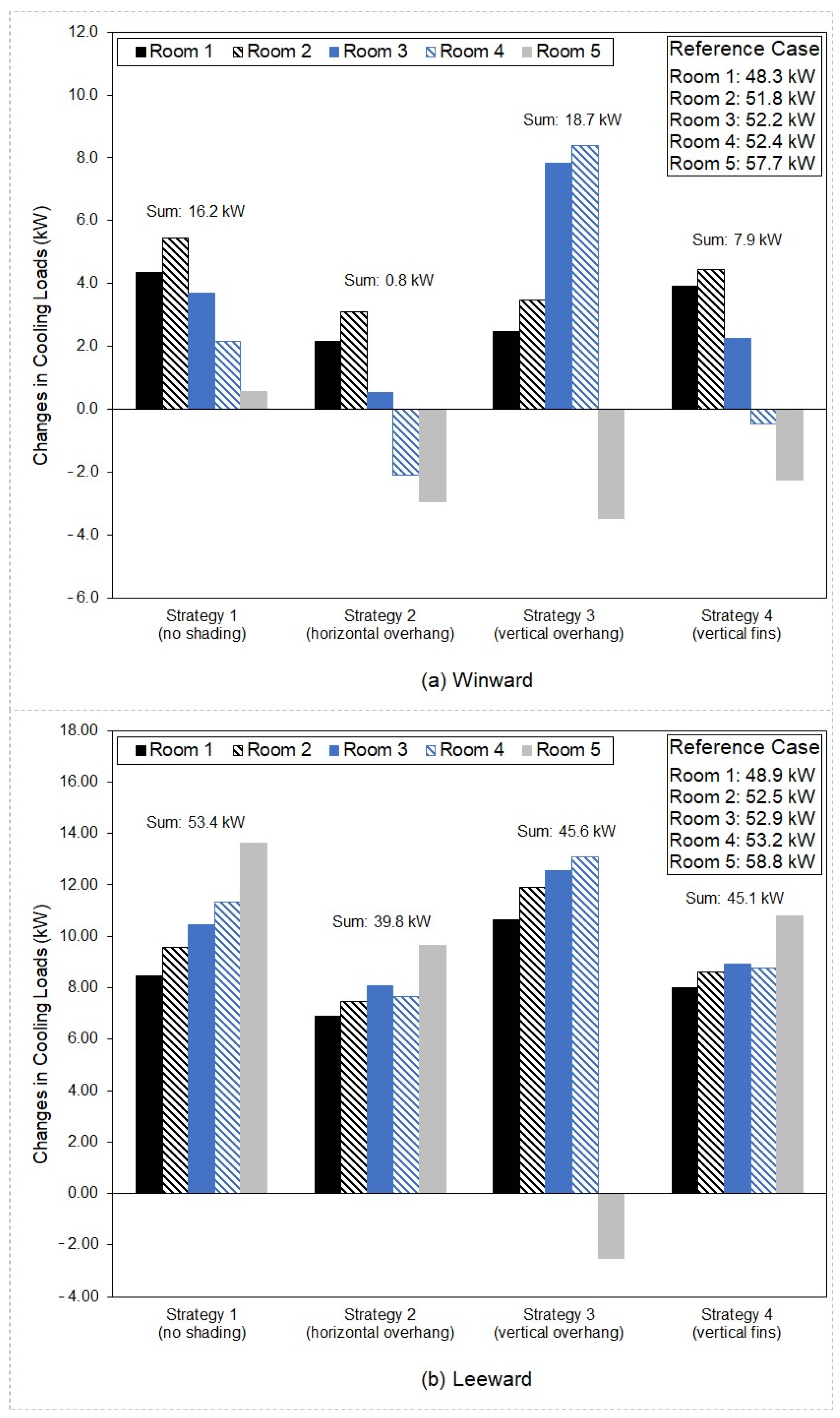
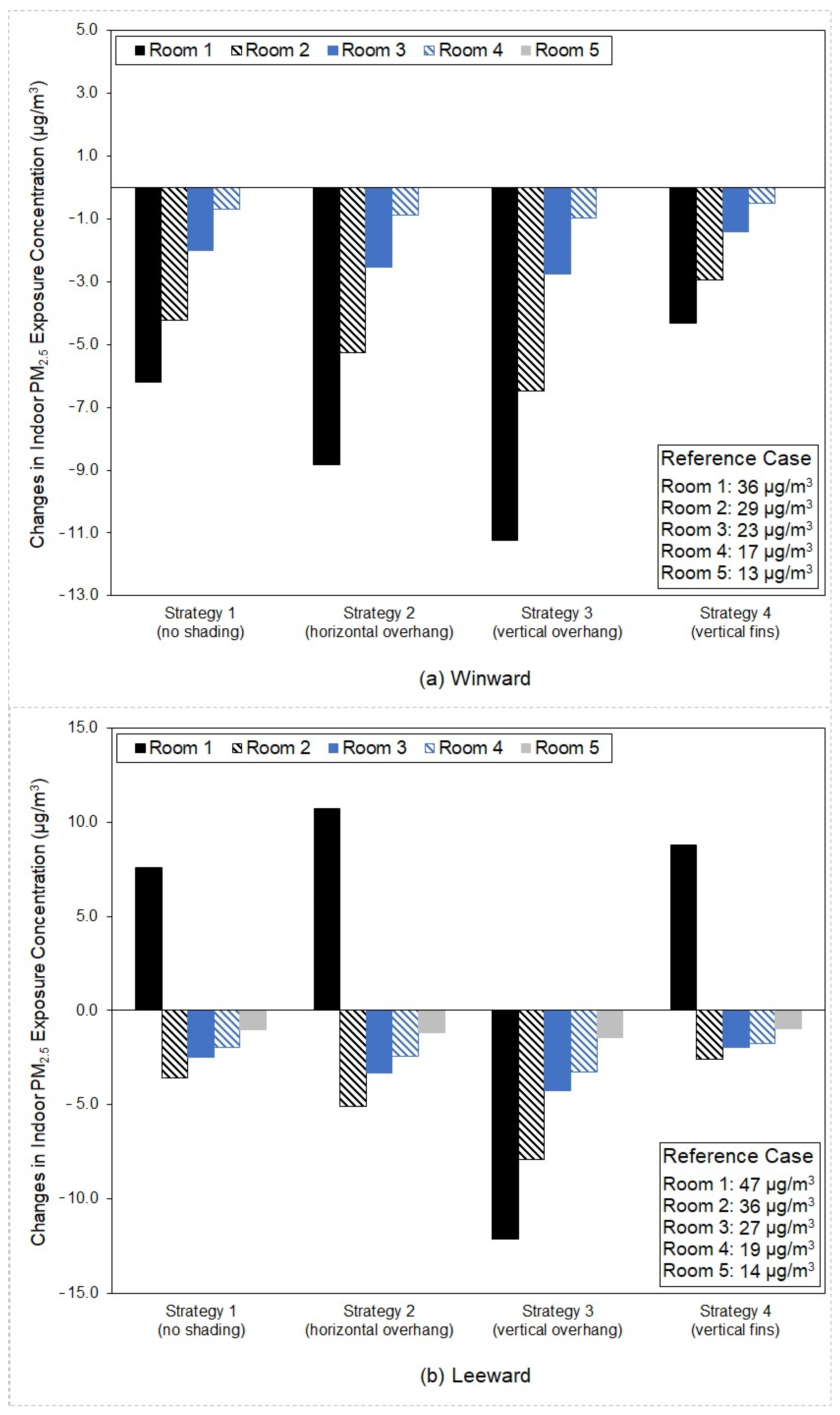
Disclaimer/Publisher’s Note: The statements, opinions and data contained in all publications are solely those of the individual author(s) and contributor(s) and not of MDPI and/or the editor(s). MDPI and/or the editor(s) disclaim responsibility for any injury to people or property resulting from any ideas, methods, instructions or products referred to in the content. |
© 2023 by the authors. Licensee MDPI, Basel, Switzerland. This article is an open access article distributed under the terms and conditions of the Creative Commons Attribution (CC BY) license (https://creativecommons.org/licenses/by/4.0/).