
Daily Carbon Assessment Framework: Towards Near Real-Time Building Carbon Emission Benchmarking for Operative and Design Insights


Abstract
:1. Introduction
2. Background
2.1. Building Energy Modelling
2.2. Digital Twin for Building Energy and Carbon Assessment
3. Methods
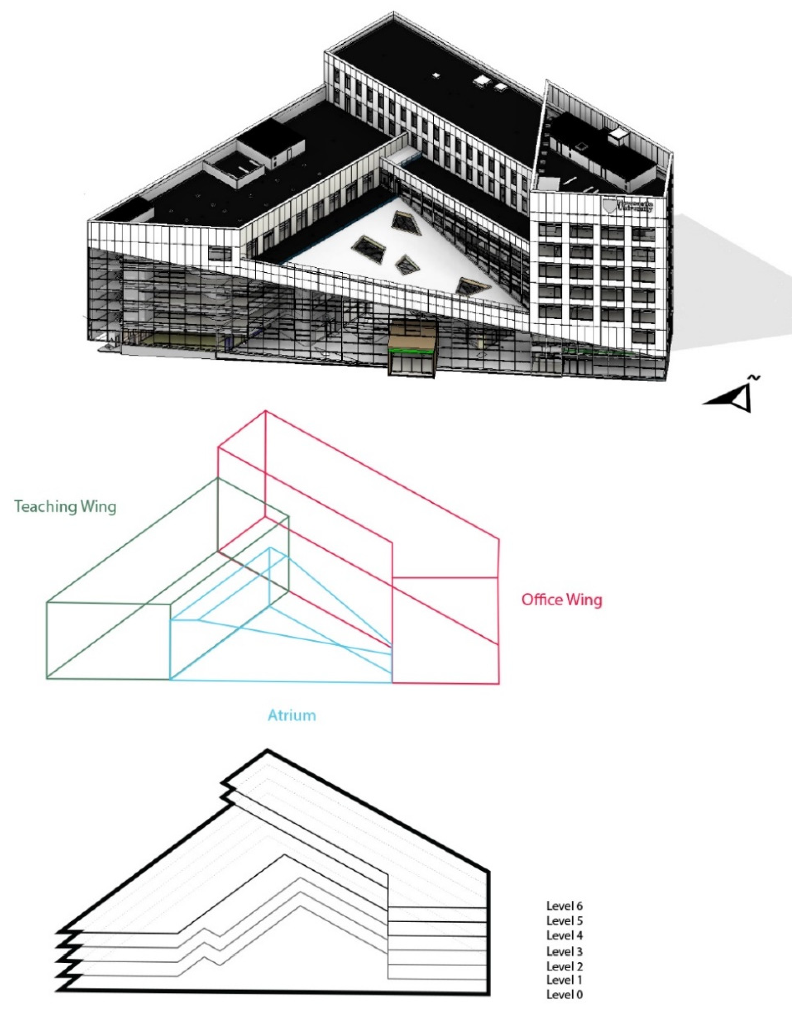
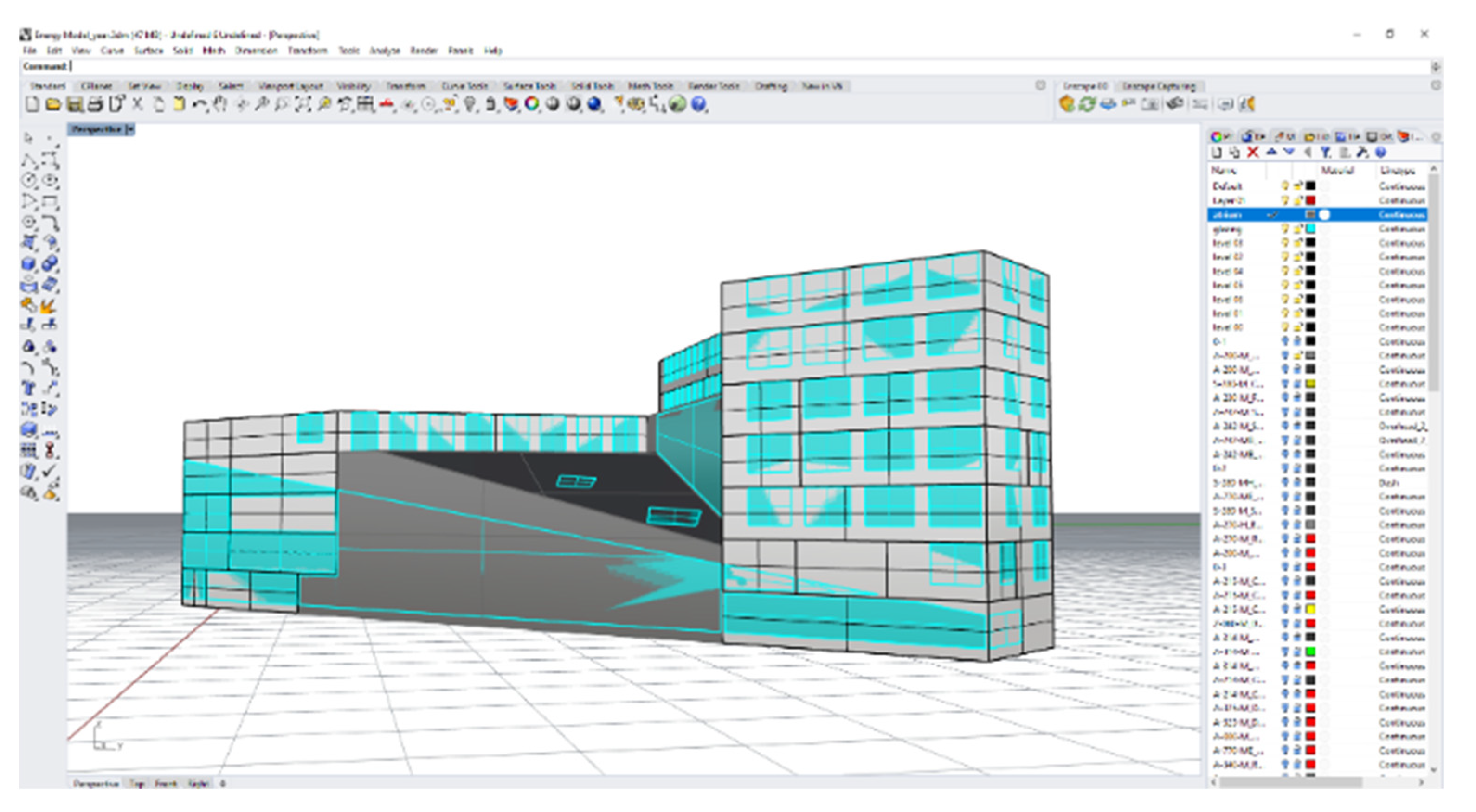
3.1. Building Description
- The availability of data including electricity consumption, on-site weather and room occupancy at a 15-min interval.
- The multi-functionality of the building is a representation of the urban dynamic at a wider context.
- It is a relatively newly constructed building that opened in September 2017. It can provide insight into the current design technology and strategy adopted.
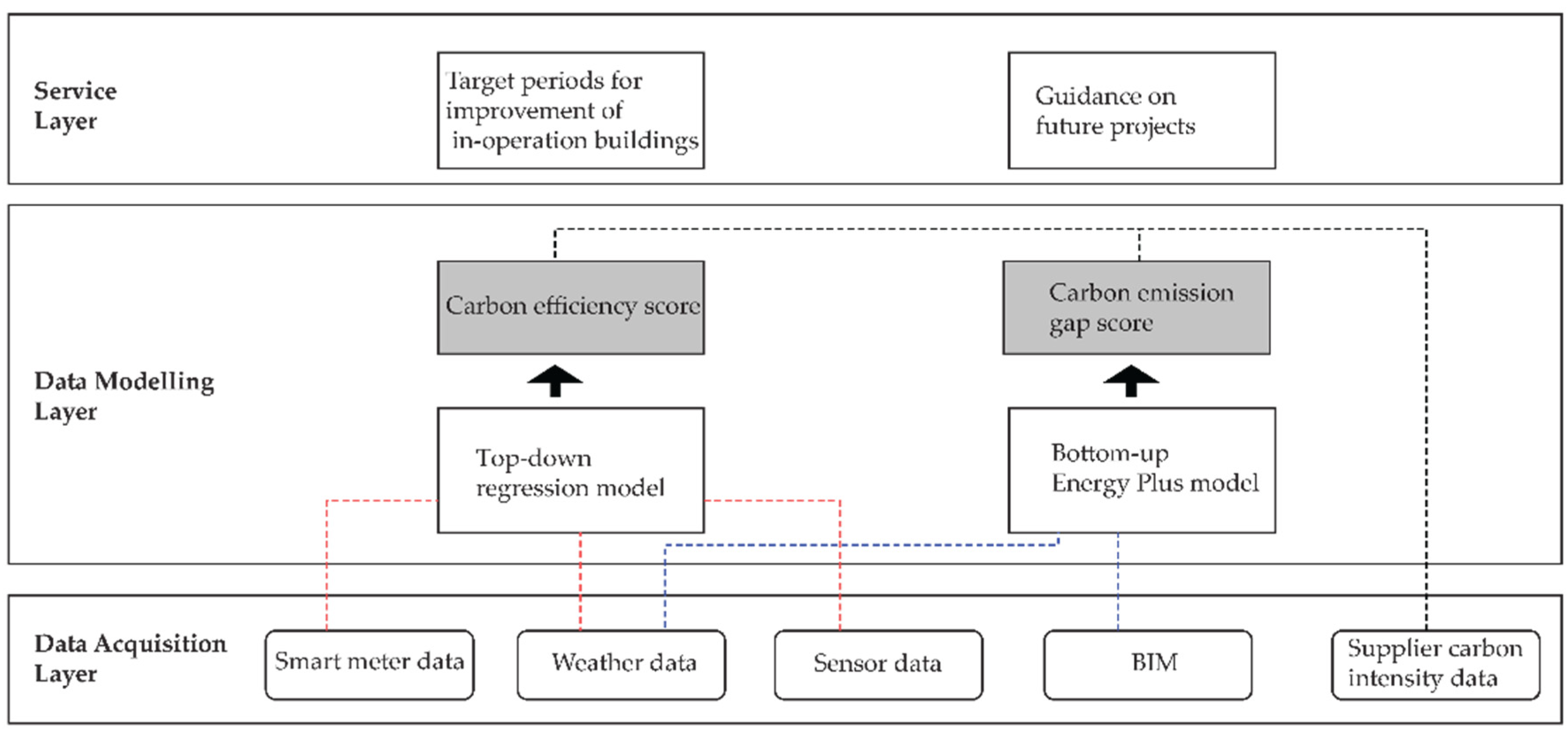
3.2. Digital Twin Framework
3.3. Segmented Time Period
3.4. Datasets
3.5. Carbon Emission Modelling
3.5.1. Top–Down Regression Model and Carbon Emission Score
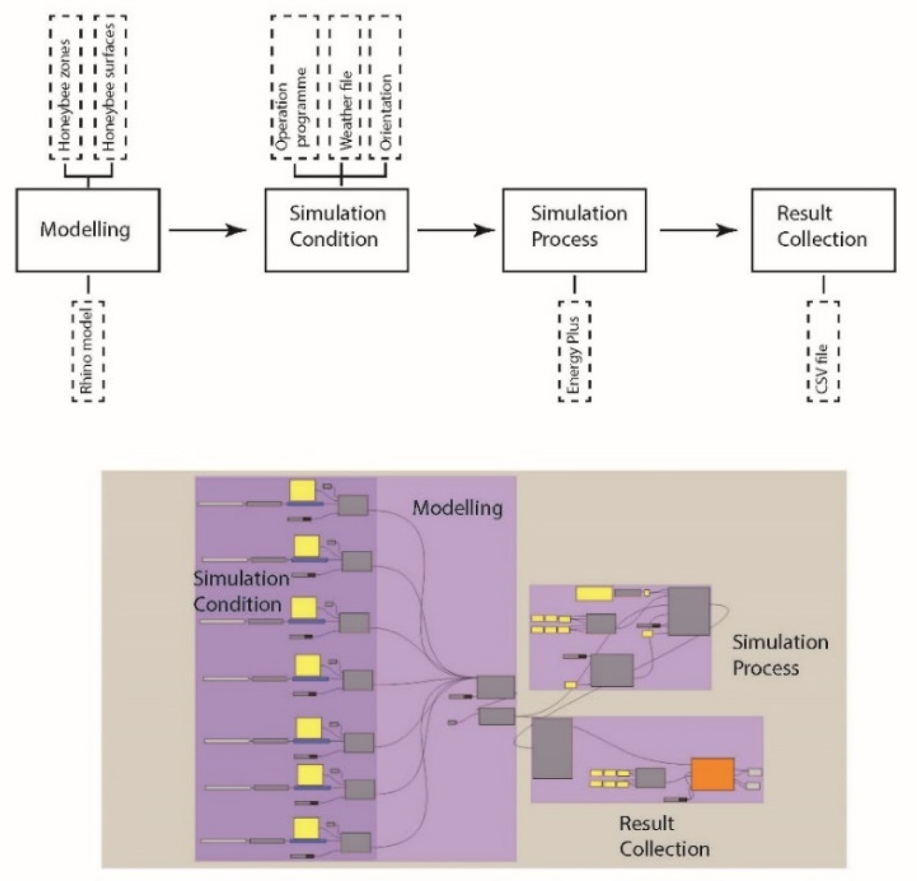
3.5.2. Bottom–Up Simulation and Carbon Emission Gap Score
4. Results
4.1. Carbon Emission Score
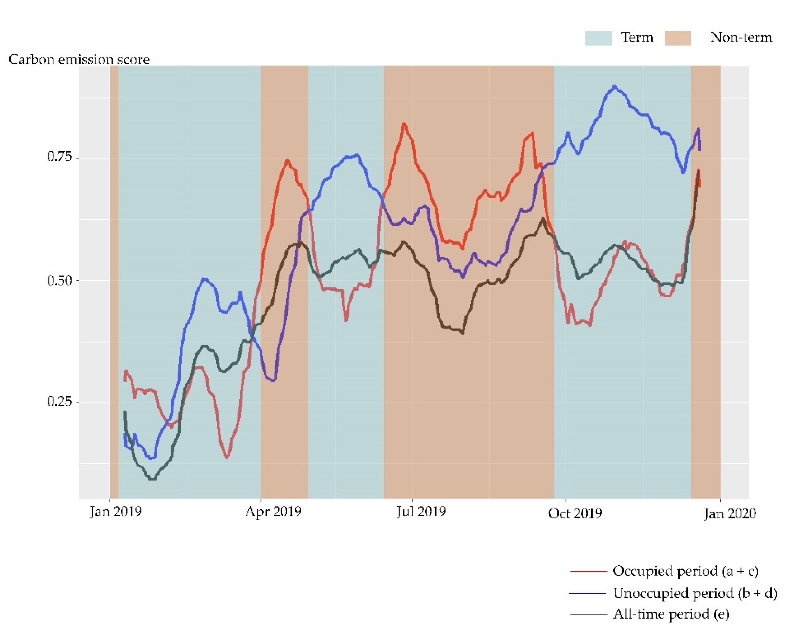
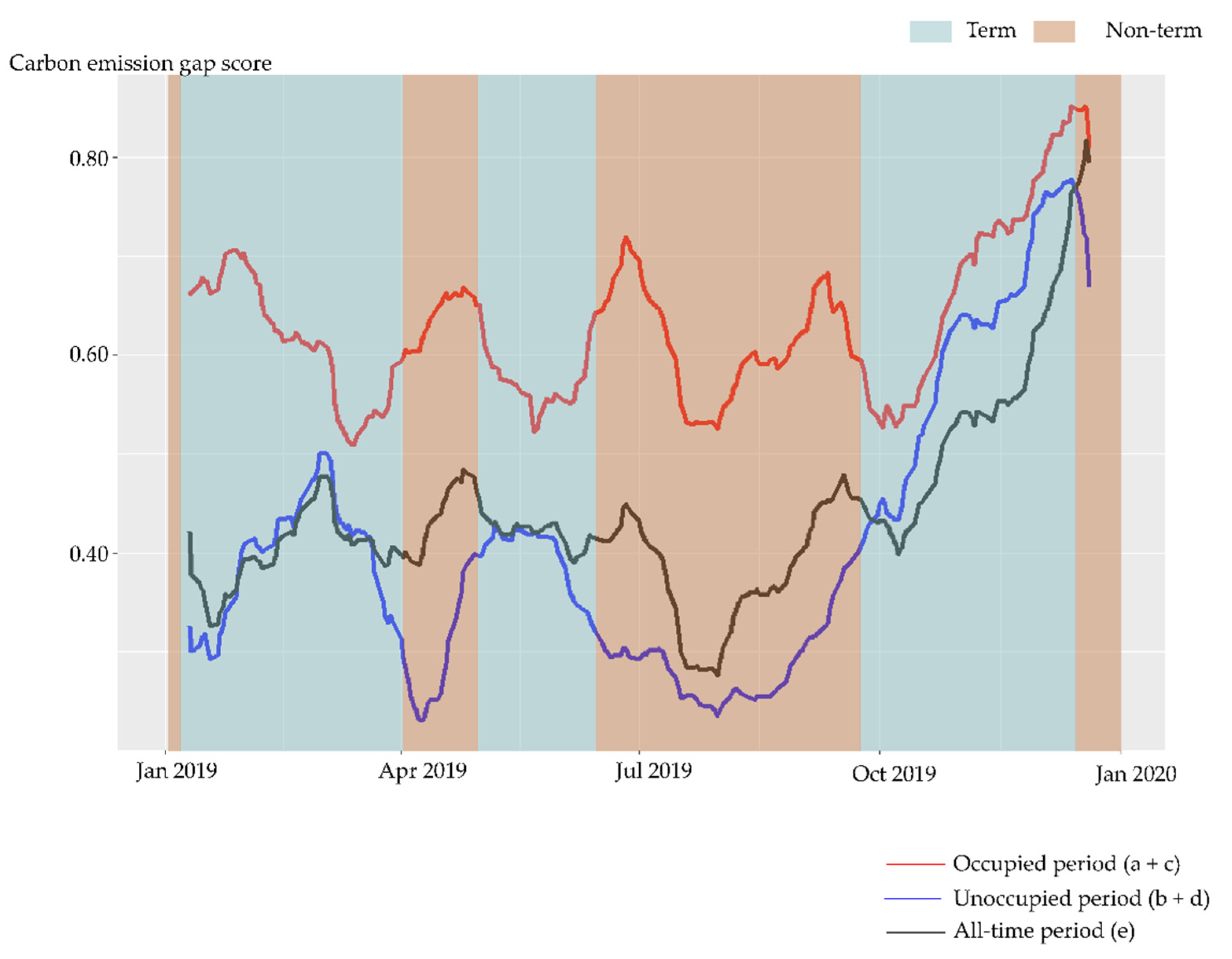
4.2. Carbon Emission Gap Score
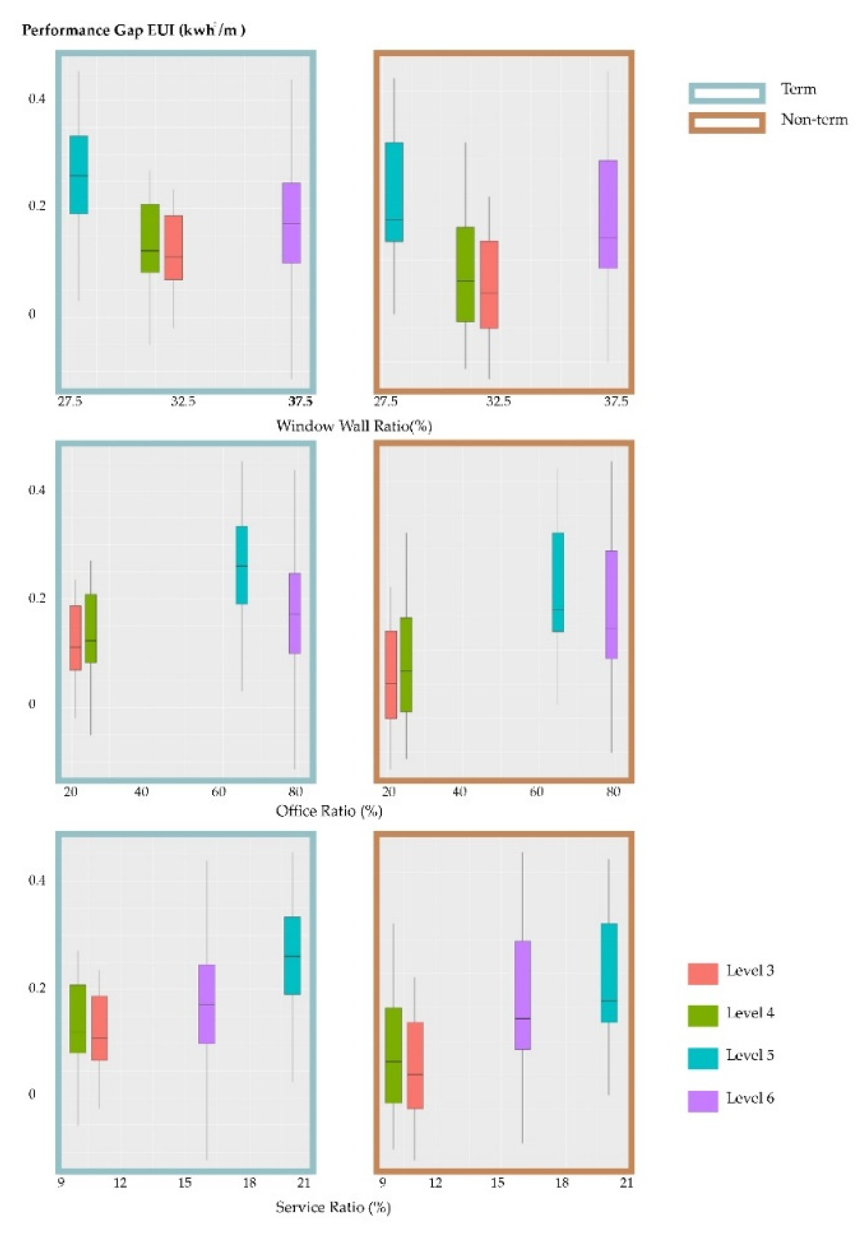
5. Service Layer
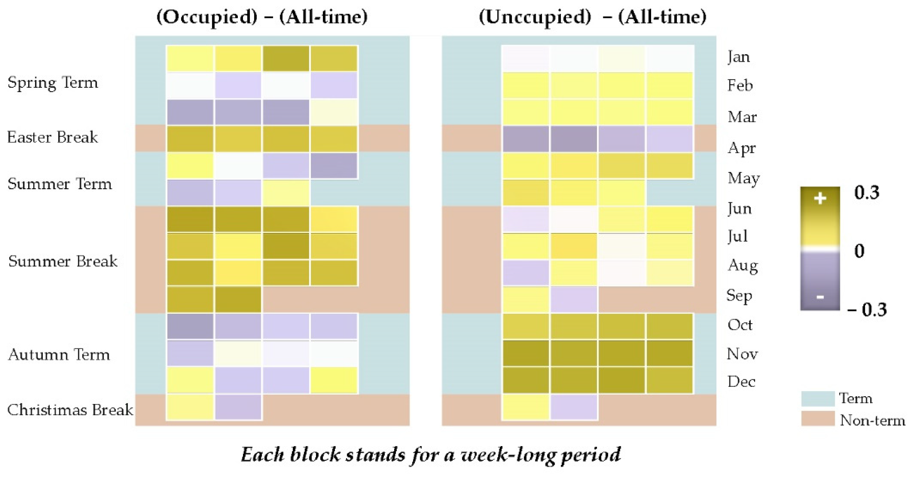
5.1. Deviation between Segmented and All-Time Periods
5.2. Insights for Future Projects
6. Discussion
6.1. Summarising the Benchmark Systems
6.2. Limitation and Future Directions
7. Conclusions
Author Contributions
Funding
Institutional Review Board Statement
Informed Consent Statement
Data Availability Statement
Conflicts of Interest
References
- Li, X.; Yao, R. Modelling heating and cooling energy demand for building stock using a hybrid approach. Energy Build. 2021, 235, 110740. [Google Scholar] [CrossRef]
- Salihi, M.; El Fiti, M.; Harmen, Y.; Chhiti, Y.; Chebak, A.; Alaoui, F.E.M.; Achak, M.; Bentiss, F.; Jama, C. Evaluation of global energy performance of building walls integrating PCM: Numerical study in semi-arid climate in Morocco. Case Stud. Constr. Mater. 2022, 16, e00979. [Google Scholar] [CrossRef]
- Borgstein, E.H.; Lamberts, R.; Hensen, J.L.M. Evaluating energy performance in non-domestic buildings: A review. Energy Build. 2016, 128, 734–755. [Google Scholar] [CrossRef]
- Metallidou, C.K.; Psannis, K.E.; Egyptiadou, E.A. Energy Efficiency in Smart Buildings: IoT Approaches. IEEE Access 2020, 8, 63679–63699. [Google Scholar] [CrossRef]
- Pärn, E.A.; Edwards, D.J.; Sing, M.C. The building information modelling trajectory in facilities management: A review. Autom. Constr. 2017, 75, 45–55. [Google Scholar] [CrossRef] [Green Version]
- Bolton, A. The Gemini Principles; Centre for Digital Built Britain: Cambridge, UK, 2018. [Google Scholar] [CrossRef]
- Lu, Q.; Parlikad, A.K.; Woodall, P.; Don Ranasinghe, G.; Xie, X.; Liang, Z.; Konstantinou, E.; Heaton, J.; Schooling, J. Developing a Digital Twin at Building and City Levels: Case Study of West Cambridge Campus. J. Manag. Eng. 2020, 36, 05020004. [Google Scholar] [CrossRef]
- Mohammadi, N.; Taylor, J.E. Smart city digital twins. In Proceedings of the 2017 IEEE Symposium Series on Computational Intelligence, SSCI, Honolulu, HI, USA, 21 November–1 December 2017; pp. 1–5. [Google Scholar] [CrossRef]
- Dawkins, O.; Dennett, A.; Hudson-Smith, A. Living with a Digital Twin: Operational management and engagement using IoT and Mixed Realities at UCL’s Here East Campus on the Queen Elizabeth Olympic Park. In Proceedings of the 26th Annual GIScience Research UK Conference: GISRUK 2018, Leicester, UK, 17–20 April 2018. [Google Scholar]
- Swan, L.G.; Ugursal, V.I. Modeling of end-use energy consumption in the residential sector: A review of modeling techniques. Renew. Sustain. Energy Rev. 2009, 13, 1819–1835. [Google Scholar] [CrossRef]
- Chung, W.; Hui, Y.V.; Lam, Y.M. Benchmarking the energy efficiency of commercial buildings. Appl. Energy 2006, 83, 1–14. [Google Scholar] [CrossRef]
- Amber, K.; Aslam, M.W.; Hussain, S.K. Electricity consumption forecasting models for administration buildings of the UK higher education sector. Energy Build. 2015, 90, 127–136. [Google Scholar] [CrossRef]
- Aranda, A.; Ferreira, G.; Mainar-Toledo, M.D.; Scarpellini, S.; Sastresa, E.L. Multiple regression models to predict the annual energy consumption in the Spanish banking sector. Energy Build. 2012, 49, 380–387. [Google Scholar] [CrossRef]
- Balaras, C.A.; Gaglia, A.G.; Georgopoulou, E.; Mirasgedis, S.; Sarafidis, Y.; Lalas, D. European residential buildings and empirical assessment of the Hellenic building stock, energy consumption, emissions and potential energy savings. Build. Environ. 2007, 42, 1298–1314. [Google Scholar] [CrossRef]
- Ang, Y.Q.; Berzolla, Z.M.; Reinhart, C.F. From concept to application: A review of use cases in urban building energy modeling. Appl. Energy 2020, 279, 115738. [Google Scholar] [CrossRef]
- Hsu, D. Identifying key variables and interactions in statistical models ofbuilding energy consumption using regularization. Energy 2015, 83, 144–155. [Google Scholar] [CrossRef] [Green Version]
- Kaewunruen, S.; Rungskunroch, P.; Welsh, J. A Digital-Twin Evaluation of Net Zero Energy Building for Existing Buildings. Sustainability 2018, 11, 159. [Google Scholar] [CrossRef] [Green Version]
- Wang, Y.; Chen, Q.; Hong, T.; Kang, C. Review of Smart Meter Data Analytics: Applications, Methodologies, and Challenges. IEEE Trans. Smart Grid 2019, 10, 3125–3148. [Google Scholar] [CrossRef] [Green Version]
- Kavousian, A.; Rajagopal, R.; Fischer, M. Determinants of residential electricity consumption: Using smart meter data to examine the effect of climate, building characteristics, appliance stock, and occupants’ behavior. Energy 2013, 55, 184–194. [Google Scholar] [CrossRef]
- Rafsanjani, H.N.; Ahn, C.R.; Chen, J. Linking building energy consumption with occupants’ energy-consuming behaviors in commercial buildings: Non-intrusive occupant load monitoring (NIOLM). Energy Build. 2018, 172, 317–327. [Google Scholar] [CrossRef]
- Roth, J.; Jain, R.K. Data-driven, multi-metric, and time-varying (DMT) building energy Benchmarking using smart meter data. In Advanced Computing Strategies for Engineering. EG-ICE 2018. Lecture Notes in Computer Science; Springer: Berlin/Heidelberg, Germany, 2018; Volume 10863, pp. 568–593. [Google Scholar] [CrossRef]
- Park, J.; Yang, B. GIS-Enabled Digital Twin System for Sustainable Evaluation of Carbon Emissions: A Case Study of Jeonju City, South Korea. Sustainability 2020, 12, 9186. [Google Scholar] [CrossRef]
- Gul, M.S.; Patidar, S. Understanding the energy consumption and occupancy of a multi-purpose academic building. Energy Build 2015, 87, 155–165. [Google Scholar] [CrossRef] [Green Version]
- Francisco, A.; Mohammadi, N.; Taylor, J.E. Smart City Digital Twin–Enabled Energy Management: Toward Real-Time Urban Building Energy Benchmarking. J. Manag. Eng. 2020, 36, 04019045. [Google Scholar] [CrossRef]
- McNeel, R. Rhinoceros 3D; Robert McNeel & Associates: Seattle, WA, USA, 2010. [Google Scholar]
- Roudsari, M.S. Ladybug + Honeybee. 2014. Available online: https://www.ladybug.tools/ (accessed on 30 June 2020).
- Bordass, B.; Cohen, R.; Standeven, M.; Leaman, A. Assessing building performance in use 3: Energy performance of the Probe buildings. Build. Res. Inf. 2001, 29, 114–128. [Google Scholar] [CrossRef]
- Nagpal, S.; Mueller, C.; Aijazi, A.; Reinhart, C.F. A methodology for auto-calibrating urban building energy models using surrogate modeling techniques. J. Build. Perform. Simul. 2019, 12, 1–16. [Google Scholar] [CrossRef]
- National Infrastructure Commission. Data for the public good. 2017, p. 3. Available online: https://nic.org.uk/app/uploads/Data-for-the-Public-Good-NIC-Report.pdf (accessed on 15 June 2022).
- Chung, W. Review of building energy-use performance benchmarking methodologies. Appl. Energy 2011, 88, 1470–1479. [Google Scholar] [CrossRef]


| Study | Explanatory Variables |
|---|---|
| [11] | Building age Occupancy Chiller equipment Lighting equipment Light control |
| [12] | Ambient temperature Solar radiation Relative humidity Wind speed Occupancy |
| [13] | Winter climatic severity Summer climatic severity Office surface area Number of employees Glazed surface in facade HAVC installed power Office height Building age |
| Period | Dates | Hours |
|---|---|---|
| Term occupied (a) | 7 January–29 March 29 April–17 June 23 September–13 December | 8:00–17:00 (M–F) |
| Term unoccupied (b) | 7 January–29 March 29 April–17 June 23 September–13 December | 0:00–8:00 17:00–24:00 (M–F) |
| Non-term occupied (c) | 1 January–4 January 1 April–26 April 17 June–21 September 16 December–31 December | 8:00–17:00 (M–F) |
| Non-term unoccupied (d) | 1 January–4 January 1 April–26 April 17 June–21 September 16 December–31 December | 0:00–8:00 17:00–24:00 (M–F) |
| All-time (e) | 1 January–31 December | 0:00–24:00 (M–F) |
| Input Parameter | Data Source |
|---|---|
| Building geometry | Revit Model CAD plan and elevation |
| Construction material | Revit Model |
| Weather condition | EPW file |
| Operational load | Building functional program |
| Period | Average Carbon Emission Gap Score (Occupied) | Average Carbon Emission Gap Score (Unoccupied) |
|---|---|---|
| Spring term (7 January–29 March) | 0.62 | 0.40 |
| Summer Term (29 April–17 June) | 0.56 | 0.39 |
| Autumn Term (23 September–13 December) | 0.66 | 0.59 |
| Easter break (1 April–26 April) | 0.56 | 0.33 |
| Summer break (17 June–21 September) | 0.62 | 0.28 |
| Christmas break (1 January–4 January and 16 December–31 December) | 0.71 | 0.69 |
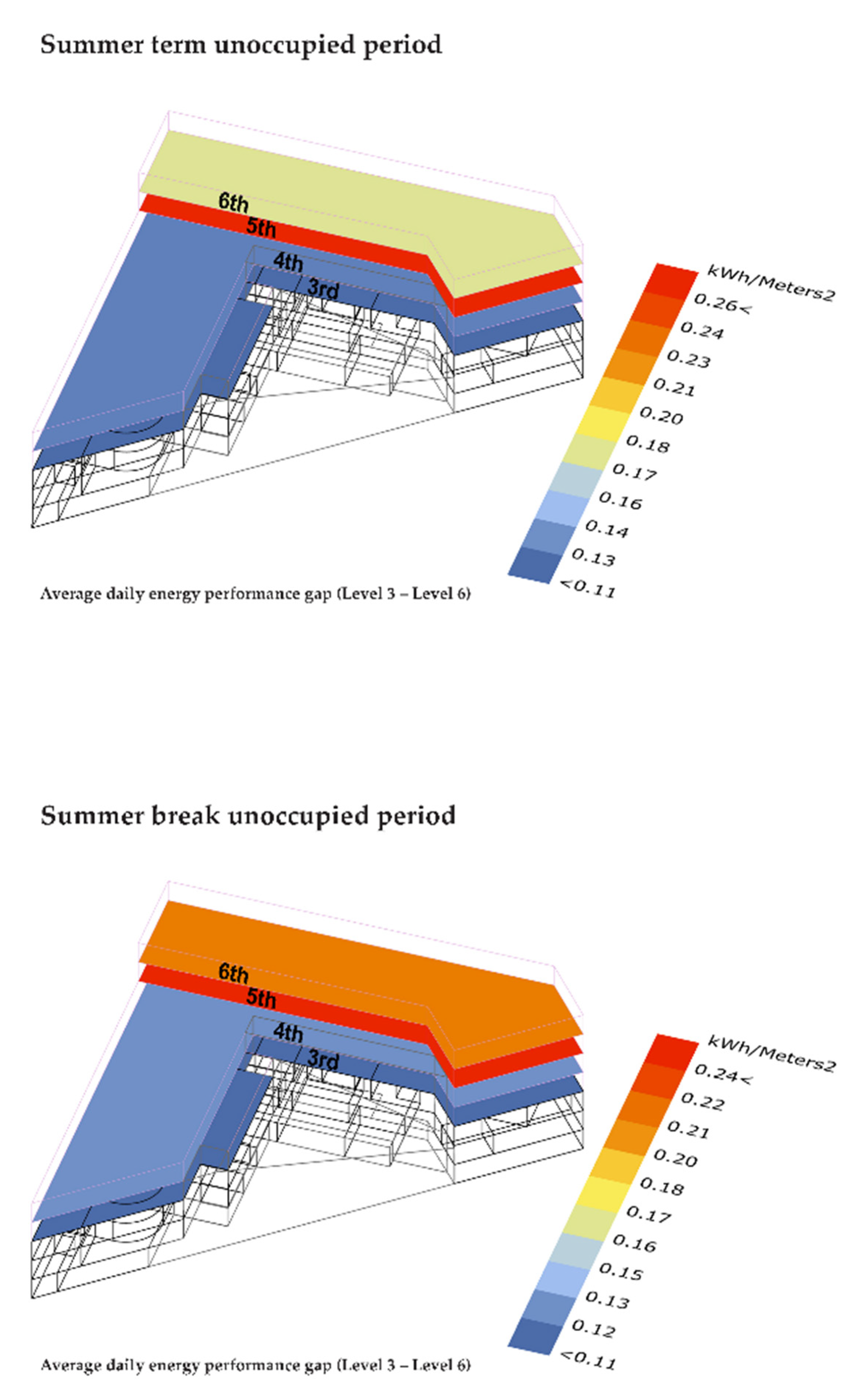
| Level | WWR% | Circulation BUR% | Office BUR% | Teaching BUR% | Service BUR% | Plant BUR% |
|---|---|---|---|---|---|---|
| 3 | 32 | 25 | 21 | 38 | 11 | 5 |
| 4 | 31 | 22 | 25 | 37 | 10 | 6 |
| 5 | 37 | 2 | 65 | 9 | 20 | 4 |
| 6 | 37 | 1 | 79 | 0 | 16 | 4 |
Publisher’s Note: MDPI stays neutral with regard to jurisdictional claims in published maps and institutional affiliations. |
© 2022 by the authors. Licensee MDPI, Basel, Switzerland. This article is an open access article distributed under the terms and conditions of the Creative Commons Attribution (CC BY) license (https://creativecommons.org/licenses/by/4.0/).
Share and Cite
Zhu, M.; James, P. Daily Carbon Assessment Framework: Towards Near Real-Time Building Carbon Emission Benchmarking for Operative and Design Insights. Buildings 2022, 12, 1129. https://doi.org/10.3390/buildings12081129
Zhu M, James P. Daily Carbon Assessment Framework: Towards Near Real-Time Building Carbon Emission Benchmarking for Operative and Design Insights. Buildings. 2022; 12(8):1129. https://doi.org/10.3390/buildings12081129
Chicago/Turabian StyleZhu, Mingyu, and Philip James. 2022. "Daily Carbon Assessment Framework: Towards Near Real-Time Building Carbon Emission Benchmarking for Operative and Design Insights" Buildings 12, no. 8: 1129. https://doi.org/10.3390/buildings12081129
APA StyleZhu, M., & James, P. (2022). Daily Carbon Assessment Framework: Towards Near Real-Time Building Carbon Emission Benchmarking for Operative and Design Insights. Buildings, 12(8), 1129. https://doi.org/10.3390/buildings12081129