Article

Guidelines to Calibrate a Multi-Residential Building Simulation Model Addressing Overheating Evaluation and Residents’ Influence

Leibniz Institute of Ecological Urban and Regional Development (IOER), 01217 Dresden, Germany
*
Author to whom correspondence should be addressed.
Buildings 2021, 11(6), 242; https://doi.org/10.3390/buildings11060242
Submission received: 22 March 2021 / Revised: 27 May 2021 / Accepted: 29 May 2021 / Published: 5 June 2021
(This article belongs to the Section Construction Management, and Computers & Digitization)

Abstract

:
Can building performance simulation reproduce measured summertime indoor conditions of a multi-residential building in good conformity? This question is answered by calibrating simulated to monitored room temperatures of several rooms of a multi-residential building for an entire summer in two process steps. First, we did a calibration for several days without the residents being present to validate the building physics of the 3D simulation model. Second, the simulations were calibrated for the entire summer period, including the residents’ impact on evolving room temperature and overheating. As a result, a high degree of conformity between simulation and measurement could be achieved for all monitored rooms. The credibility of our results was secured by a detailed sensitivity analysis under varying meteorological conditions, shading situations, and window ventilation or room use in the simulation model. For top floor dwellings, a high overheating intensity was evoked by a combination of insufficient use of night-time window ventilation and non-heat-adapted residential behavior in combination with high solar gains and low heat storage capacities. Finally, the overall findings were merged into a process guideline to describe how a step-by-step calibration of residential building simulation models can be done. This guideline is intended to be a starting point for future discussions about the validity of the simplified boundary conditions which are often used in present-day standard overheating assessment.

1. Introduction

The projections on global warming predict a strong increase in the frequency and severity of heat waves for the next decades, even for scenarios of quickly and efficiently realized climate protection measures on a global scale [1]. In connection with the fact that people in industrial nations spend over 80% of their time in buildings [2] the impact of a predictable and already noticeable increase of summer temperatures on overheating in buildings becomes particularly relevant. In the past, for most moderate climate zones passive cooling measures, like adequate window ventilation had been sufficient and could avoid the use of active mechanical cooling that would cause further greenhouse gas emissions. The critical question arises if the present building stock, not designed for increasing summer temperatures and urban heat islands effects [3], will be capable of ensuring sufficient thermal comfort in the future or if adaptation measures to the buildings, or even mechanical cooling systems are inevitable.
One way to evaluate overheating in buildings is to use thermal building performance simulation (BPS). In the last few years, a significant increase in the number of publications using this method for overheating evaluation was recorded (summarised by Chen (2019)) [4], predominantly originating in Great Britain. As for many kinds of simulation, the question arises if the simulation results reflect the real situation in a sufficient manner. Uncertainties for BPS are based on the correct choice of boundary conditions, especially concerning user behavior, building physics or meteorological data.
Scientific publications of overheating analyses commonly focus on investigating the impact of boundary conditions on the overheating risk solely using BPS without validation by recorded room temperature measurements [5,6,7,8,9,10,11], while detailed studies utilising room temperature measurements for overheating evaluation without considering BPS can be found as well [12,13,14,15]. Some studies applied both, measurements and simulation, but were not able to calibrate their simulation to measured room temperatures, because the meteorological dataset used in their simulation did not represent the meteorological conditions of the summer period where the building comfort monitoring was performed [16,17]. An attempt to calibrate the simulated to the measured room temperature time series carried out by Mavrogianni et al. failed in consequence of unknown occupant behavior [18]. McLeod et al. (2017) and Mourkos et al. (2020) successfully calibrated indoor thermal condition monitoring and building performance simulation, but only considered chronical overheating, meaning overheating of buildings of more than 26 °C indoor temperature in times of cool weather below 20 °C outdoor air temperature was mainly caused by mistakes in the building design or during operation [19,20,21,22]. Roberts et al., tested a comprehensive method to calibrate a free running 3D model of two synthetically occupied detached houses [23]. However, even using different simulation programs, the monitored daily temporal evolution of the room temperatures was much lower in intensity between day and night compared to the simulation. Summarizing the literature research, we find that investigation on conformity of simulated to monitored room temperatures are rare for residential buildings and mostly exhibit non-negligible differences between measurements and simulations.
Besides developing a detailed and credible 3D model of the building, an important factor to achieve a sufficient model calibration to real measurements is based on a reliable implementation of the user behavior [24]. Concerning the evaluation of overheating, it is known that internal heat gain profiles caused by occupants and their window ventilation behavior are crucial parameters [15]. However, window ventilation is commonly only implemented as formally specified in standards for overheating assessment like CIBSE TM 59 or DIN 4108-2. These standards do not consider a wind or temperature gradient driven interzonal air exchange, and only assume constant air exchange rates when windows are opened.
The present article suggests an approach to achieve high conformity of simulation and reality by calibrating simulated room temperature to monitored data of several rooms in an exemplary multi-residential building in Germany. The required wind and temperature gradient driven air exchange is considered in the chosen BPS program. Compared to previous literature, the comparison of monitored and simulated room temperatures was performed for a whole summer period and not only for several days or weeks. In addition, not only were the monitored rooms simulated, but the entire building including all dwellings to consider infiltration paths and thermal conductivities between dwellings and rooms through ceilings, internal walls and room doors. In this paper, we demonstrate a step-by-step process to calibrate simulated to monitored summer-time overheating of a multi-residential building using BPS and to what extent the residents’ behavior influences the overheating intensity.

2. Methods

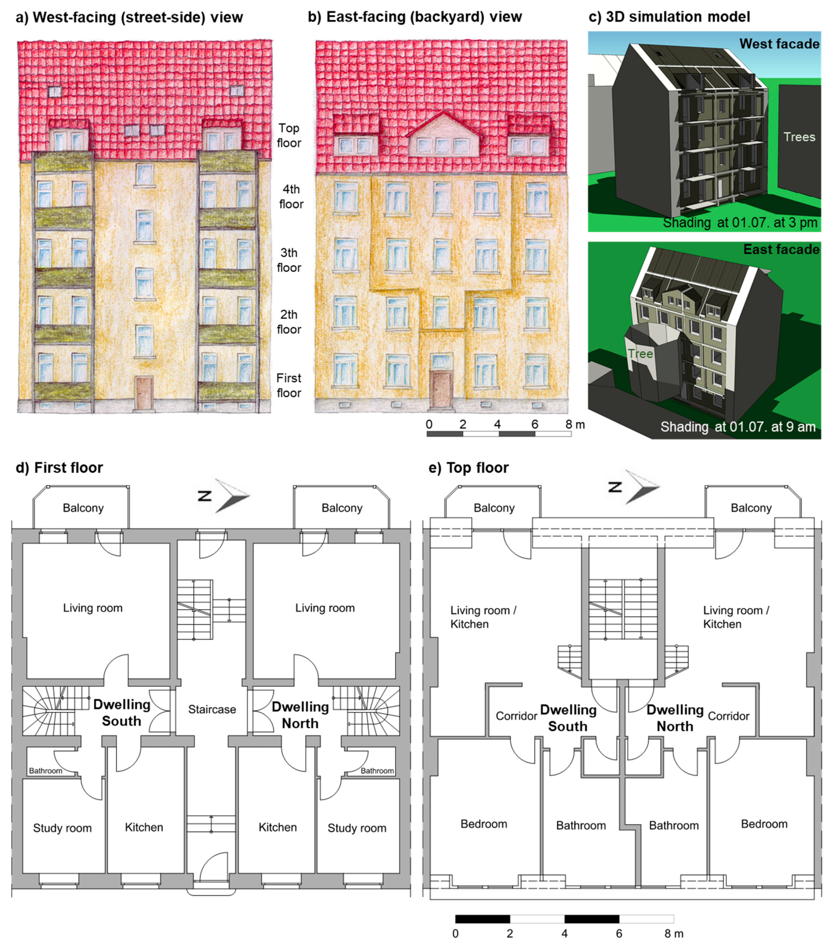
2.1. Building Properties

Buildings in large cities are more affected by summer heat than in the rural areas caused by the urban heat island effect [25]. For this reason, a multi-residential building type, frequently represented in larger European cities were selected for this overheating analysis. The “Gründerzeithaus” (GZH), erected in the turn of the 20th century in the center of Erfurt (Germany), was chosen. The side views and floor plans of the chosen GZH example building are depicted in Figure 1. Because the building is arranged in block edge development, similar neighborneighboring buildings are connected to the GZH at the north and south side. Characteristics for such building types are their thick, uninsulated brick walls with rendered façade, the saddle roof with dormers as well as wooden beam ceilings between the individual dwellings. The investigated building consists of two dwellings on each floor (only rooms in the 1st and 2nd floor are connected to a single dwelling), four full stories, and a converted attic, giving a total net floor area of 725 m2.
To facilitate reliable overheating evaluations by BPS, a detailed research of the building components including building documents, on-site visits, and further investigations were performed. The building structure components including their corresponding heat transfer coefficients are listed in Table 1. The thick exterior and interior brick walls of the GZH building provides high thermal storage capacities, helping to mitigate extreme indoor temperatures in summer. However, the rooms in the converted attic dwellings exhibit low thermal storage capacities because of the installed drywall constructions for internal walls. In addition, the external walls in the attic are insulated from the internal to enhance the thermal insulation. The well-insulated roof reduces the overheating risk due to a low transmittance of solar heat gains from the dark-red colored roof surface. The consideration of solar shadings is an important issue concerning overheating analysis by BPS. For the GZH balconies on the west (backyard) façade, the awnings of the attic dwelling as well as the surrounding trees were considered. The neighboring building on the east (street) side was also taken into account. The shadow cast caused the by surrounding buildings, balconies, and trees is depicted in Figure 1c. For the 1st floor dwellings, the basement of the building induces a limited cooling effect. The suspended wooden beam ceilings with a low U-value leads to low transmittance between dwellings of different stories and exhibit a low heat storage capacity.

2.2. Indoor Measurements

In the summer period of the year 2019 (from 3 June to 7 October), indoor monitoring was performed for ten selected rooms. All residents were tenants of this building and were recruited through a letter distributed by the property management with the request to participate in the project. The process of conducting surveys in advance, installation and collection of the monitoring sensors (stand alone with battery operation) was designed and performed together with social scientists, a data protection commissioner, the property management of the building as well as the municipality (which was also involved in the project) and tested in multi-stage procedures. In order to increase the motivation of the residents to participate in the monitoring program, it was pledged in advance to present and discuss the outcomes in retrospect. This was carried out in an on-site user training workshop after the monitoring had been evaluated. The indoor air temperature, the relative humidity and the CO2 concentration for most rooms were recorded with a time-resolution of 5 min. For this purpose, the autonomous data logger DK660 (including CO2-measurement) and DK320 (without CO2-measurement) from the company Driesen+Kern GmbH® were positioned in the individual rooms at positions that solar irradiation and internal heat gain does not affect the indoor measurements. The measurement uncertainty for room air temperature is +/− 0.1 K. The equipment was provided and calibrated by the University of Applied Sciences of Dresden. Ten rooms were equipped with data loggers, measuring air temperature and CO2 concentration (8) or solely temperature (2). The rooms are located in
  • 1st floor/ground floor: Study room (east) and living room (west)
  • 2nd floor: Children room (east) and sleeping room (west)
  • 4th floor: Bedroom (east) and kitchen-living room (west)
  • 5th floor/attic: both dwellings each with bedroom (east) and kitchen-living room (west)

2.3. Local Meteorological Data

High conformity between simulated and measured room temperature time series can only be achieved if local meteorological data with resolution of at least one hour is available. Especially outdoor air temperature and wind properties differ significantly between urban centers and their surroundings, but also within the urban structures. For the city of Erfurt, the nearest certified meteorological station from the German Meteorological Service (DWD) is Erfurt-Bindersleben [26], located 6 km western from the GZH building. However, the station is situated nearby the airport, and thus located 100 m higher than the city center of Erfurt. Hence, the wind and outdoor temperature values are not representative for the GZH building, located in the valley basin of Erfurt.
For this reason, a THIES DLX® temperature data logger was installed in the nearest possible location of the GZH building, which was a shaded green area in a distance of 550 m, to gain a more representative meteorological outdoor air temperature input for the BPS. The recording started at 13 May 2019 and ended on 15 October 2019 with a temporal resolution of 10 mins.
For the required wind speed and wind direction data, recorded measurements from the meteorological station “Bautzener Weg”, operated by the Office for Environment, Mining and Nature Conservation of the Federal State of Thuringia were selected [27]. The station is located on an open field 1.7 km north-eastern from the GZH building and monitors wind speed and wind direction in a 10 m height. Thus, the station displays more representative wind conditions for the GZH building location than the DWD station Erfurt-Bindersleben, located outside the valley basin of Erfurt. However, wind measurements directly nearby the building would be more accurate, but contrary to the outdoor air temperatures, it was not possible to realize measurements near the building site. To address this uncertainty, the sensitivity of wind speed and wind direction data from the station “Bautzener Weg” and Erfurt-Bindersleben on differences in air exchange in the building was investigated. A comparison of the selected wind and outdoor air temperature data input for the building from the station “Bautzener Weg” with the data from the DWD station Erfurt-Bindersleben (in the environs of Erfurt) in Figure 2 shows strong differences in night-time cooling and wind speed. Characteristic outdoor temperature and wind values in Table 2 accentuate a 1.5 K higher maximum and mean summer temperature and a lower wind speed in maximum and mean value for the meteorological data input used for the GZH building.
In addition to outdoor air temperature and wind conditions, representative direct and diffuse solar irradiation with time resolution of at least 1 h are required for BPS. However, the next meteorological station of the DWD recording solar irradiation data is located in more than 100 km distance to the GZH building. Fortunately, the Office for Environment, Mining and Nature Conservation of the Federal State of Thuringia operate two pyranometers at their location in the city of Jena, situated 40 km western from the GZH building in Erfurt [28], recording both direct and diffuse irradiation. The diffuse and direct solar irradiation profile was successfully proven by a comparison of the daily temporal evolution of direct and diffuse solar irradiation to other certified DWD weather stations in the surroundings. However, it is important to mention that differences between the solar irradiation in Erfurt and Jena can occur for several hours, especially for days with variable cloudiness. The global irradiation of the station in Jena in Figure 2 demonstrates a high number of sunny days for the summer of 2019.
Summarizing, the created meteorological data set used for the BPS consists of outdoor air temperature measurements near the GZH building, wind speed and wind direction measurements in a 1.7 km distance (without disturbing building objects) and direct and diffuse solar irradiance measurements at a distance of 40 km.

2.4. Building Performance Simulation

For the simulations of the GZH building the BPS software IDA ICE 4.8® [29] was used (Validation history of IDA ICE: http://www.equaonline.com/iceuser/new_validationreports.html (accessed at 29 October 2020)). The simulations were run for an entire year at a time step of less than one hour to allow detailed analysis of the evolving air temperatures for each room. A preconditioning period of one month was applied. Building components and material layers are implemented as inputs to reproduce realistic heat storage and heat transmission dynamics.
The following standard boundary conditions were applied for BPS:
  • Location of the building is Erfurt, Germany
  • Orientation of the building similar to reality (east-side façade oriented to the street, west-side oriented to the backyard)
  • Shading objects on the GZH building were taken into account, e.g., the building on the opposite side of the street (east façade), balconies on the west-side façade as well as shading of trees on the street-side, and in the backyard (cf. Figure 1c).
  • Sun protection systems: For the actual GZH building, no external sun protection systems are present, and thus considered.
  • Thermal bridges: Overall thermal bridge loss coefficient of 0.10 W/(m2K) is related to all component surfaces according to DIN 18599-2 for existing buildings without internal insulation [30].
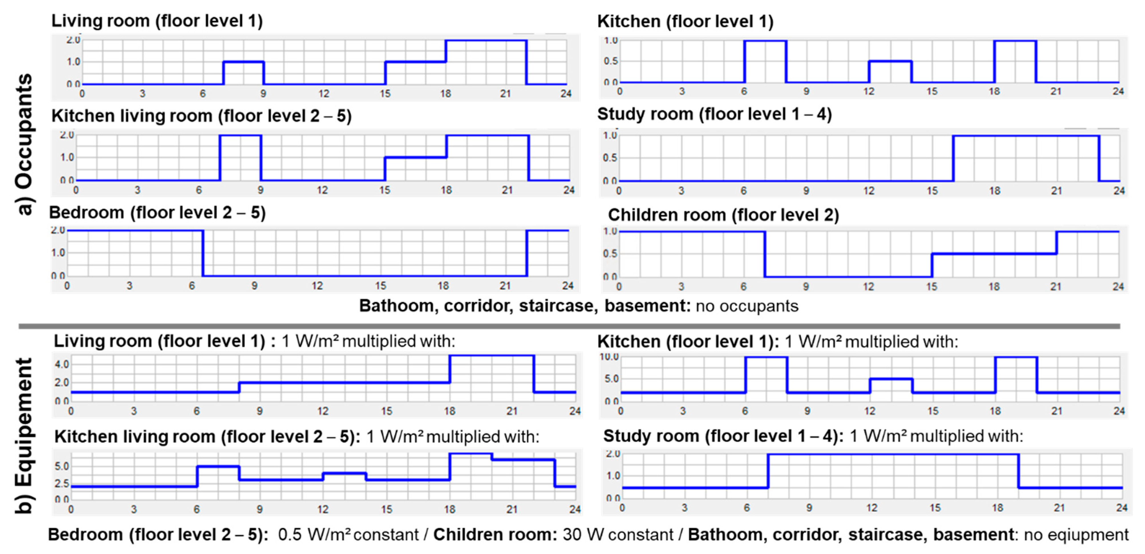
  • Internal loads: The daily time series of the initial internal heat loads for the investigated ten rooms and the internal loads for all (neighboring) rooms (set for all simulation variants) are depicted in Figure A1 of the Appendix A. The presence and number of occupants for the dwellings were derived from a residents’ survey conducted in the selected GZH buildings and answered by the residents of five of eight dwellings. In this survey, the following issues have been asked: number and age of residents, common presence of occupants during a day, the kind and use of window shadings (curtains and for the top floor dwellings awnings for the western-faced rooms; external sun protection systems are not installed), if nocturnal window ventilation is commonly applied as well as cross ventilation. Because of privacy protection, the operation of electrical devices in the dwellings could not be monitored. However, the results of the survey showed, that most residents are median age living together with 1–2 children and work apart during the day, although not all surveys were answered entirely. The derived internal heat gain profiles are only rough assumptions because room uses vary individually for different dwellings. The impacts of internal heat gains on overheating intensity of rooms are discussed in the sensitivity analysis.
  • Air exchange (window opening and infiltration) by wind and temperature gradient is included in the BPS software IDA ICE; to gain high accordance between measured and simulated room temperatures, the air exchange of rooms caused by window ventilation and infiltration driven by wind and temperature gradients must be represented as realistically as possible for the calibration by BPS. IDA ICE enables this opportunity to take into account wind flows through a building by considering pressure coefficient of the individual façade and roof elements. Thus, wind-driven interzonal air exchanges in the building as well as cross ventilation by opening room doors can be considered in BPS. Besides these wind-driven air flows, temperature gradient driven air exchange by different indoor to outdoor or adjacent room temperatures is considered as well. The wind and temperature gradient driven infiltration is calculated by IDA ICE by defining an n50 (air exchange rate at 50 Pa pressure coefficient) value of 2 h−1 (according to DIN EN 15242 for average leakages) as a measure of air tightness for the GZH building. A more detailed description of the air exchange algorithm can be found in the Appendix A (“multizonal air exchange calculation in IDA ICE”).
  • Window openings for all rooms in the GZH building (except the individual investigated ten monitored rooms) are defined as follows:
    Window opening control: windows opened when the outdoor air is cooler than the room air, and the room air > 22 °C (depending on the window opening schedule)
    Window opening schedule: windows are fully opened from 6 p.m. to 10 p.m. and 6 a.m. to 7 a.m.; tilted during the night from 10 p.m. to 6 a.m.
    Degree of window opening: taken from measurements of the existing opening area of the installed windows
    All room doors remain closed
This assumed and simplified window ventilation behavior is an outcome of a previous article [31]. However, window ventilation shows a large impact on evolving room temperatures, but a variation in window opening behavior revealed that the impact of the neighboring rooms to the monitored ten rooms is relatively small for the GZH building type.

2.5. Overheating Criteria

Room temperature time series and maximum room temperatures only give a rough impression about the overheating risk and intensity. Indicators, which include the maximum and the duration of room temperature above an acceptable temperature threshold, are more suitable to evaluate the heat burden in a room. However, no universally accepted international definition and criteria for an overheating indicator for buildings is currently available [4].In Germany, overheating assessment is commonly done using the national standard DIN 4108-2 [32]. For Erfurt, the acceptable comfort temperature (operative temperature) threshold is defined as 26 °C. This upper boundary is used to calculate the so-called “overtemperature degree hours” (ODH) as a measure of overheating within the rooms of a building for an entire year. For residential buildings, an upper limit for ODH of 1200 Kh/a (Kelvin hours/annum) is defined for acceptable overheating intensity. Besides the ODH, overheating indicators according to EN15251 [33] and CIBSE TM59 [34] are used in the literature, especially in the UK [16,35]. Their advantage is that they do not use a fixed threshold value for the room temperature, but that this depends on the outdoor temperature, i.e., taking into account human adaptation. However, in this method only the number of hours of exceedance above the adaptive temperature limit is taken into account, not the maximum of exceedance at a certain time. Both, strength and the duration of overheating are only implemented in the ODH method. For this reason, the ODH indicator was chosen for the present study.
It is important to mention, that boundary conditions used for our investigations like detailed window ventilation behavior, using measured meteorological data and implementing room use depending on internal heat gain difference from the simplified boundary conditions defined in the standard DIN 4108-2. Thus, attention must be paid when discussing absolute ODH limits in relation to our investigations. To compare measured and simulated temperature temporal evolution, the simulated room air temperature is also used instead of the operative temperature.

3. Results and Analysis

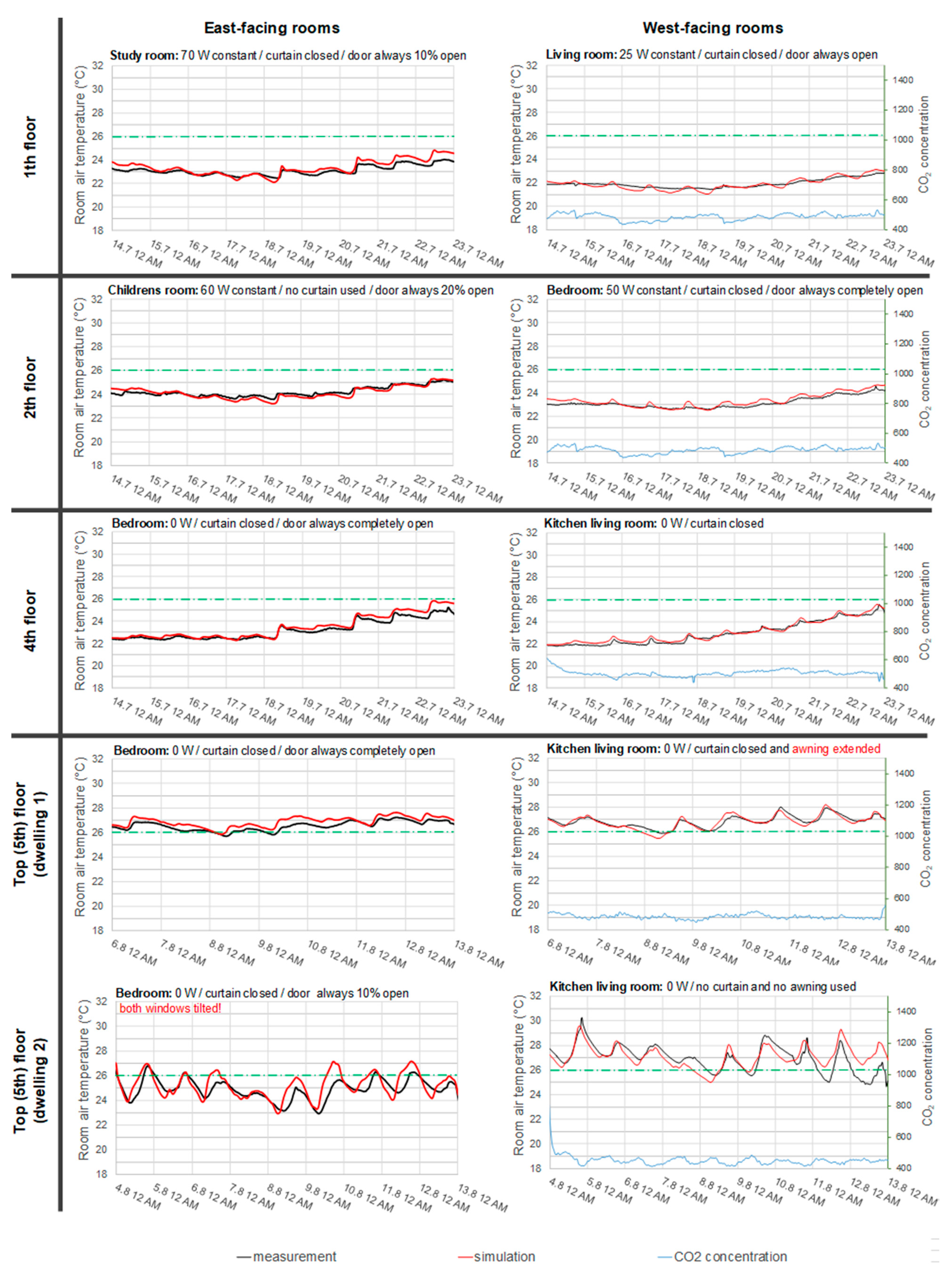
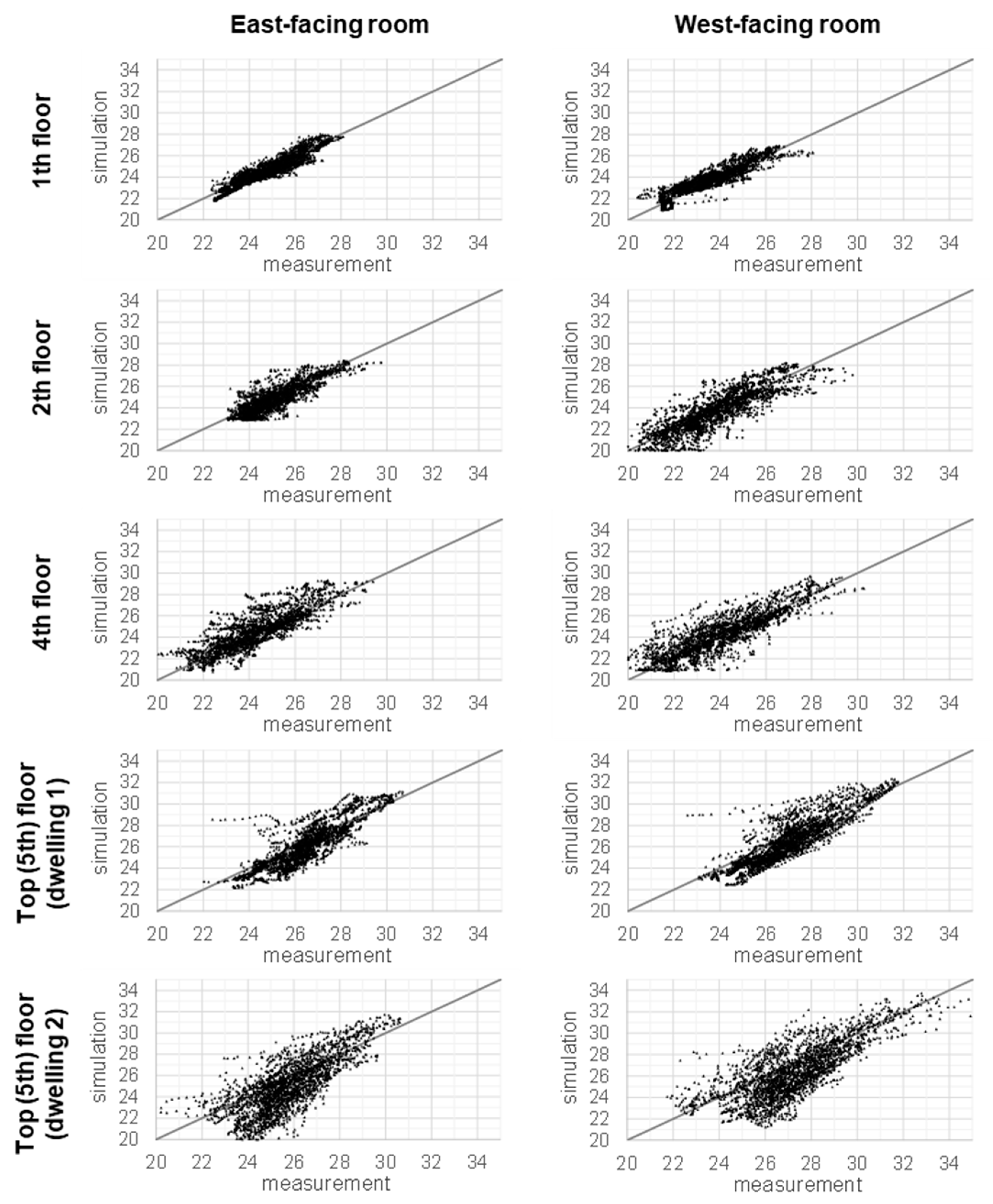
3.1. Monitoring Results

The resulting room temperature as well as the CO2 concentration time series of the monitoring period are depicted in Figure 3 and point out two important issues. First, the room temperatures of the western oriented rooms are in general comparable to the rooms on the eastern side, and frequently exceed the thermal comfort temperature threshold of 26 °C. Second, the CO2 concentration of the eastern oriented rooms is much higher than on the opposite western side. The latter can be explained by the different room uses. While the western oriented rooms are mostly large kitchen- living rooms (except for the 2nd floor), the eastern oriented rooms are much smaller with a higher and longer occupancy, especially in the bedrooms with two persons in the 4th floor and attic. However, CO2 concentrations much above 1000 ppm in the warm summer period were not expected and are a first hint that window ventilation is not used sufficiently.
Compared to the full stories, the converted attic dwellings show significantly higher room temperatures, especially for the kitchen-living rooms on the west side. For the attic, the monitoring in both architecturally comparable dwellings offered the opportunity to reveal what differences in obtained room temperatures can be traced back to individual residential behavior. The comparison of both attic dwellings in Figure A2 of the Appendix A clearly demonstrates significant differences in the temperature curves, especially in the homogeneity of the temperature time series. Simulating the GZH building with BPS can reveal the origin of these differences and especially help to analyze if the overheating is caused by insufficient heat resilience of the GZH building or by occupant behavior.

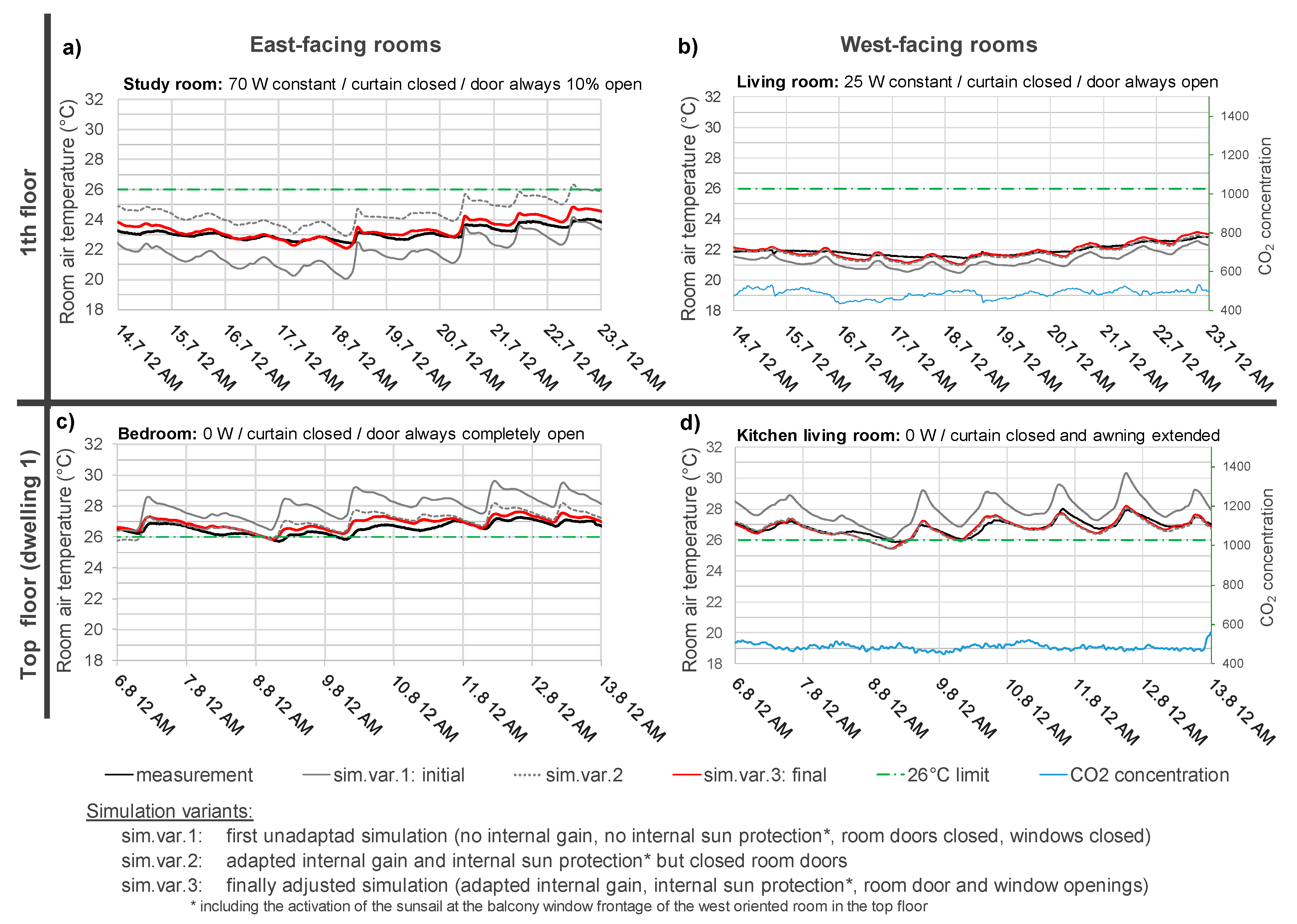
3.2. Simulation Adjustment in the Absence of Residents

The CO2 concentration measurements were performed for most monitored rooms and allow to determine time spans when no occupants were present in the dwelling for several days. For this time period, the room temperature is not influenced by actions of the residents and thus the evolving room temperatures in the dwelling only depend on the building physics. This enables the opportunity to prove the correctness of the 3D building simulation model of the GZH, i.e., regarding realistic window sizes and glazing, realistic thermal transmittance through the building envelope, reliable absorption values of the building envelope and realistic heat storage behavior. Figure 4 compares the monitored and simulated the room temperature temporal evolution for the time period where no residents were present in the first and top floor dwelling (visible by the low CO2 concentration of around 400 to 500 ppm). To convey the stepwise way to the high conformity of simulated to monitored room temperature time series, three simulation variants are depicted representatively describing the calibration steps:
  • The first variant represents the initial simulation run without implementation of any internal gains or internal sun protection and with closed windows or room doors. The simulated temporal development of temperature run fairly parallel to the measured ones, but for most rooms with stronger variations within the day.
  • In the second variant internal solar shading via the use of curtains (reduction factor of solar gain Fc = 0.7) was applied for most rooms, as well as constant internal heat gain by electrical devices to achieve better conformity with the measured room temperature. The measured temperature time series in the kitchen-living room of the attic dwelling can only be matched if the awning, installed by the tenants on top of the huge window front, is extended and shades the room.
  • In the third variant, final calibration of the simulation model was conducted by implementing the effect of open room doors. Especially for the study room in the 1st floor, a remarkable impact of air exchange can be observed as caused by the small room size combined with high solar and internal heat gains.
While Figure 4 shows four selected example rooms of calibrations, Figure A3 (see Appendix A) depicts the measured and calibrated simulated room temperatures for all ten monitored rooms for a time-period of occupants’ absence. For all rooms a high conformity between monitored and simulated room temperatures was achieved. The simulation parameters for each individual room of the calibrated simulation variant are written above each diagram in Figure 4 and Figure A3. For the bedroom of dwelling 2 in the attic (cf. Figure A3), the temperature time series only shows good conformity between measurement and simulation if both small windows are assumed to remain tilted during the absence of the residents. These partly opened windows lead to more pronounced fluctuations in room temperature compared to the other nine monitored rooms with closed windows.
Summarising, to gain high conformity between monitored and simulated room temperatures for the time spans of the residents’ absence, it is vital to display the solar gain into the room realistically (g-value and size of the glazing area or shadings), to consider internal gains by running electrical devices and to observe an air exchange to neighboring rooms by open doors. As discussed in Section 4.3, the relatively small internal gains defined for the individual rooms to gain good calibration can also be caused by heat transmittance from neighboring dwellings, where the real room temperature is unknown because no monitoring was performed there. Nevertheless, the results demonstrate that the thermal transmittance of the building envelope, solar heat gained through windows and especially thermal storage capacities in the 3D model of the GZH building are reproduced realistically.

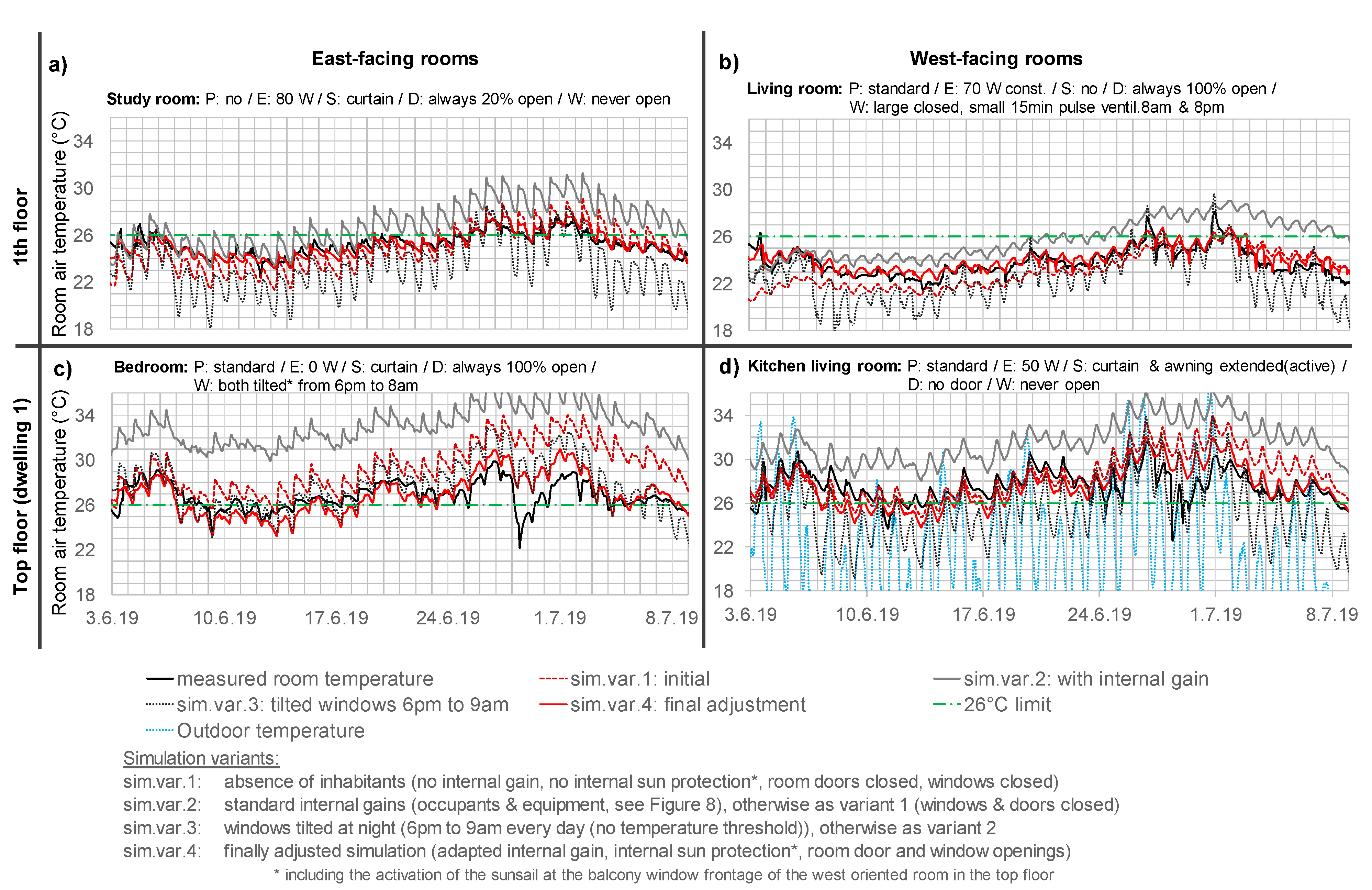
3.3. Simulation Adjustment Including Residents’ Behavior

After validation of the 3D simulation model in time spans of residents’ absence, the complete monitoring time period is simulated as the next step—including the impact of residents’ behavior. To gain high conformity of simulation to reality, a step wise variation of residents’ behavior in the BPS process was conducted. The process is depicted in Figure 5 for the simulated room temperature temporal evolution of the 1st and the top floor dwelling exemplarily.
The initial BPS variant reveals similar simulated and measured room temperature time series if no resident presence (no internal heat gain, no window ventilation) is assumed for the whole time period. In contrast, applying internal heat gains by residents and equipment of a standard room use (according to Figure A1, Appendix A) while windows remain closed in the second variant, indicates a significant shift of around 3 K higher simulated temperatures, but with intraday temperature variations remain similar to variant 1. This scenario of room use without any air exchange is unrealistic, and is the reason for the large obtained deviation of measured and simulated room temperatures. In the next step, variant 3, a standard window ventilation is assumed in addition to the internal loads acquired from variant 2. In this simplified scenario, all windows are tilted during the night (from 6 pm until 9 am), independent of the outdoor air temperature (room doors remain closed). As a result, the simulated room temperature lowers, and those intraday room temperature differences increase, caused by the cooling effect of the limited air exchange through tilted windows. However, both changes are too strong compared to the measured time series, indicating a lower ventilation intensity than assumed. To achieve better calibration, window opening intensity and duration as well as room door opening behavior are varied in a final step. Simulation variant 4 results in high conformity of simulation and measurement. The varied boundary conditions for the individual rooms of the final simulation variant 4 are written above the diagrams in Figure 5.
This step-by-step calibration process of varying the residents’ behavior was performed for all ten monitored rooms as depicted in Figure 6. To compare the resulting conformity in numbers, both mean and maximum room temperatures as well as ODH of measurement and simulation are juxtaposed in Table 3. The root mean square error (RMSE) for the measured to the simulated room temperature and ODH are derived as indicators for calibration conformity. In addition to the RSME, plots of measured (monitored) room temperature to simulated room temperature profiles in Figure A4 (Appendix A) reveal no bias for all monitored rooms of the GZH building. Although, both RSME as well as the scattering intensity of values in the measured-simulated room temperature plots rise with increasing floor level, this increase is originated in the more pronounced room temperature daily cycles observed for higher floors, inducing larger deviations between measured and simulated temperature courses. In summary, a good calibration quality was achieved for all rooms, although a very simplified user behavior (like window and room door opening, presence of the residents, or use of internal sun protection) was applied to be the same each day for the entire simulation period. This outcome is discussed in Section 4.2 in more detail.
For several days, the residents’ behavior deviated from our assumed “mean” behavior, leading to peaks in monitored room temperature, which are not possible to comprehend with our simplified approach of equal behavior each day. An example for this effect can be found on 30 June 2019 for top floor dwelling 1 (cf. Figure 5). Here, the windows were opened for a much longer time span, leading to a significant room temperature drop in reality, compared to the low ventilation behavior used in the simulation, which is suitable to trace the measured temperature temporal evolutions during most times of the monitoring period. Another example can be found for the kitchen-living room of the top floor dwelling 2 (cf. Figure 6). A deeper analysis reveals that the high maximum measured room temperatures of more than 36 °C (25 and 26 June 2019) were caused by windows opened in the afternoon when outdoor air temperatures of more than 37 °C were obtained. In the simulation, the window was closed during the whole day, which is a suitable assumption to gain a high degree of conformity for the other times of the monitoring period. These deviations in measured and simulated maximum room temperatures are also visual in Table 3 for the kitchen-living room of the top floor dwelling 2, located at the west façade. The maximum room temperature of this room would be around 34 °C, and not the measured 36.7 °C when the window of this room would remain closed during this hot afternoon.
Table 3 also displays a significant difference in overheating intensity between the dwellings in the developed attic, and dwellings located in the full-stories. As already mentioned, the intense overheating of the attic can be traced back to deviations in building physics compared to the full stories: low heat storage capacities (drywall construction) combined with a high solar heat gain through the roof and the unshaded (no balcony) large windows on the western façade and the roof windows as well. However, comparing both attic dwellings with identical construction properties, different room temperature time series can be obtained in Figure 6 with higher daily fluctuations in room temperature for dwelling 2. This can be traced back by deviations in residents’ behavior as an outcome of calibration of the BPS model to measurements: First, the BPS results show that awning of the large balcony windows seems to be not extended in the kitchen-living room for dwelling 2, leading to higher solar heat gain and thus stronger room temperature increase during the day. Second, the windows of the bedroom of dwelling 2 are partly fully opened during the night and not only tilted as in dwelling 1. In combination with open room doors this difference leads to the obtained enhanced room temperature drop during the night and increase during the day. However, the overheating intensity for both dwellings is comparable (see similar ODH in Table 3) because higher solar heat gains are compensated by a better window ventilation during the night in dwelling 2. These findings raise the question what effect user behavior and building properties have on the overheating risk of dwellings, which is highlighted in the next section.

3.4. Sensitivity of Overheating

In the process of calibrating simulations to measurements, several boundary conditions with significant impact on the simulated room temperature time series were obtained. In advance of the demonstrated calibration process, the impact of several other parameters, which had insecurities in its assumption on the evolving simulated room temperature were tested, e.g., temporal evolution and maximum number of present occupants and electrical appliances, effects of different internal shading systems and especially the impact of window and room door opening profiles. The (one factor at a time—OAT) sensitivity analysis presented here only shows a small excerpt of over 200 simulation variations done to ensure the chosen parameters set for the final model calibration were as trustworthy as possible. Five different parameters with high impact on evolving simulated room temperature are depicted in Figure 7 with corresponding ODH values in Table 4. In these simulation variants, only one parameter was varied while all the others remained the same to the final calibrated simulation variant 4 (cf. Figure 6). The following boundary conditions were varied:
(a)
Meteorological data input:
As described in Section 2.3, the outdoor air temperature profile was taken from measurements within the district of the GZH building on a shaded green area and wind data was selected from measurements in less than a 2 km distance for all simulation variants. To examine the significance of meteorological data on simulation results, the wind and outdoor air temperature data from the DWD meteorological station at Erfurt-Bindersleben was applied. This station is located 6 km western and 100 m higher than the city center of Erfurt, and thus results were higher in wind speed and lower in outdoor air temperature (cf. Figure 2). The BPS showed that the impact of evolving room temperature on outdoor air temperature is significant, leading to a room temperature decrease of more than 1 K when the data from the DWD station (cf. Figure 7) is used and correspondingly a strong decrease in overheating—expressed by halving of the ODH in Table 4. In contrast, the effect of the different wind speeds is much lower, which is caused by the low degree of window opening in the final simulation variant (cf. Figure 6). The impact of meteorological conditions on overheating highlights the necessity to use local meteorological data near the simulated building for calibrations. Also, it demonstrates that the same GZH building with the same residents’ behavior would result in a much lower overheating intensity for rural regions than in the city center, mainly attributed by worse night-cooling within the urban area.
(b)
Surrounding shading objects (buildings, trees, balconies):
Figure 1c shows how the shading situation of the investigated GZH building by trees (one tree at East façade, row of trees in the South-East), by surrounding buildings (on the opposite to the east façade), and by balconies (at the western façade) is represented in the 3D simulation model. In Figure 7, the impact of neglecting these shading objects on evolving simulated room temperatures in the 1st floor dwelling is shown. The neighboring buildings as well as the balconies especially show a strong impact on evolving room temperatures, but the absence of the trees has a noticeable impact as well. While shading by trees and neighboring buildings only affects the first floors of the building, the balconies (and the awning used for dwelling 1 of the attic) are important shading elements for all stories. The comparison of the ODH in Table 4 demonstrates that the absence of trees does not directly affect the higher floors but only indirectly by transmissions between the different stories to a small extent. If the neighboring building would not be present, the ODH of the east oriented rooms would increase from the 1st to the 4th floor, leading to critical overheating intensities for the not ventilated small study room in the 1st floor. As expected, the omission of the awning in the kitchen-living room of dwelling 1 in the attic would also induced a strong increase in ODH. The adjacent bedroom (air exchange by room door open) and the neighbored dwelling 2 (heat transmissions through the walls) are also affected to a small extent. In sum, the individual shading situation of the building plays a vital role and needs to be considered in BPS in an accurate manner. These lead to limitations to transfer the results of the overheating analysis of one building to another of the same type but with different shading situations.
(c)
Room use (quarantine scenario):
The time of presence, the occupancy density as well as the use of electrical equipment can affect the overheating intensity. Therefore, we varied the intensity of the use of dwelling 1 in the attic by the scenario of a quarantine of the residents, becoming more realistic since the COVID-19 pandemic. In all presented results so far, the residents were absent from home during the day (see Figure A1, Appendix A). In contrast, in the quarantine scenario, it is assumed that two adults and one kindergarten child were present during the whole day in their dwelling. One adult is assumed doing home office in the bedroom and the other adult is taking on childcare with the infant in the large kitchen-living room. Some windows are tilted during the day to guarantee fresh air supply. The detailed applied resident behavior can be found in Table A1 of the Appendix A. Two different simulation runs were performed, one run with closed bedroom door, during the time of home office to be undisturbed, and one run with open bedroom door. In Figure 7, the changes in evolving room temperature for the quarantine scenarios are depicted. While the large kitchen-living room is not significantly affected by different room use caused by its size, the rise of the room temperatures in the small bedroom is tremendous, leading to critical overheating situations during home office times, especially when the bedroom door remains closed. For all days the bedroom temperature rises above 27 °C and up to 34 °C when the bedroom door remains closed, which is problematic to perform concentrated work in there. This strong overheating intensity is caused by the mixture of large internal heat gains and solar gains combined with a low heat storage capacity and low room volume of the small bedroom. The result clearly demonstrates the dependence of overheating risk on the individual room use situation, especially for small rooms.
(d)
Window ventilation behavior:
For buildings in Central European climate with chilly nights (summer outdoor temperatures below 20 °C), the cooling potential for dwelling during the night by window ventilation is high. However, in the investigated GZH building the potential of night-time ventilation is used insufficiently as (except for one dwelling) simulation calibration leads to the results that windows were only tilted in the bedrooms, and remain closed in most living rooms during the night (cf. Figure 5). Even for the significantly overheated top floor dwellings, the big window front of the kitchen-living room seems to remain closed in the evening and during the night during hot spells. To demonstrate the large potential of night-time cooling, simulation scenarios were performed in which the windows of the bedrooms were fully opened during the night, whereas windows at the balconies were only tilted in the GZH building (except windows in 1st floor which remained closed owing to the risk of burglary). The room doors were closed in the first variant and opened in the second one to analyse the effect of cross-ventilation. The detailed window and room opening conditions and the comparison to the standard ventilation conditions can be found in Table A2 (Appendix A). The simulated room temperature time series for the top dwelling in Figure 7 highlights the remarkable effect of window ventilation during the night by a room temperature decrease of around 2 K for the bedroom (windows fully open during night) and around 1 K for the kitchen-living room (windows are only tilted during night here). For cold nights, room temperature drops up to 8 K could be obtained from the evening until next morning. This is in good agreements to room temperature monitoring performed for another GZH building with well-recorded window ventilation behavior. The strong decrease in overheating due to night-time ventilation is also expressed by lower ODH values in Table 4 compared to the standard scenario (final calibration to measurements). The impact of cross ventilation on room temperature is unexpectedly low. From other PBTS studies, we found that cross ventilation can increase the air exchange rate significantly and thus leads to an enhanced cooling effect [31,36]. However, caused by the assumption that the balcony French window is only tilted during the night, the air exchange by cross ventilation is significantly limited. Therefore, especially during hot periods, the full potential of cross-ventilation through fully opening windows at night is recommended, if possible.
(e)
Sun protection:
Besides adaptation of the individual user behavior, several constructive adaptation measures can be realised to reduce solar heat transmissions through sun exposed roof surfaces and window glazing. The impact of sun protection is shown in two scenarios, first by installation of a photovoltaic system on the roof leading to a shading of the roof surface, and second by installation of external sun protection systems (Fc = 0.2 for bedroom and Fc = 0.3 for kitchen-living room) for all windows of the attic dwellings. As an outcome, the shading effect of the photovoltaic modules on the roof leads to around 1 K cooler room temperatures in the top floor dwelling (Figure 7) and accordingly to a perceptible reduction of ODH in Table 4. In comparison, the second scenario of implementing external sun protection systems is found to be even more effective resulting in a much slower room temperature rise during the day and thus up to 4 K cooler room temperatures in the top floor dwellings. The impact on ODH reduction in Table 4 is comparable to the optimized window ventilation scenario (d). This clearly demonstrates that both, constructional and behavioral adaptation measures can lead to a vital reduction in overheating risk. Another interesting aspect could be obtained for the reference scenario (e) in Table 4 for the top floor dwelling 1, where awning and curtain were removed. Here, the ODH raised to values above 4000 Kh/a, which highlights the tremendous overheating risk for the top floor dwelling when a combination of high solar gains and low window ventilation behavior are present.

4. Discussion

4.1. Conformity of Simulated to Monitored Room Temperatures

In Section 3.2 and Section 3.3, the stepwise process to gain high conformity of simulated to monitored room temperatures for an entire summer period are presented considering all rooms of an entire multi-residential building. This result might be vitally important to the BPS society because it demonstrates that BPS can display the reality of overheating in buildings in a good quality, and even more, help to analyse the realistic user behavior. In our literature research (see introduction part), no study was identified with such a high conformity between simulation and result, especially not for an entire summer period.
In the process of calibration, the initial simulation run including all building physics information available for the GZH (cf. Figure 4) led to an accurate reflection of the monitored rooms in the absence of residents. Only the use of curtains, open room doors and small constant heat gains originated by electrical appliances or heat transmission from neighboring dwellings needed to be calibrated. Much more effort was required to achieve a good conformity of simulation and measurement when residents’ presence was included with their associated window ventilation, room door opening, and heat gains by persons and electrical equipment (cf. Section 3.3). The results of the calibration process as well as the sensitivity analysis in Section 3.4 demonstrates that the type of window ventilation and room door opening are the most sensitive variables. In present overheating assessment standardisations like CIBSE TM 59 in the UK or DIN 4108-2 in Germany (DIN4108 2013, CIBSE 2017), the implementation of window ventilation is very much simplified by constant air exchange rates. Our findings underline that natural ventilation is vital to be implemented in a realistic manner in BPS including wind and temperature gradient driven air exchanges.

4.2. Impact of Residents on Overheating

The conformity of simulation to measurement was restricted by the simplified assumption made for simulations, especially that resident behavior (internal heat gain, window and room door opening) is set to be identical for each day over the entire investigated time period of the summer 2019. Thus, outdoor air temperature dependent window opening, and variations in the presence of residents e.g., on weekends were neglected. However, the good conformity of measurement to simulation in Figure 5 and Table 3 indicates that this simplified assumption might be sufficient. Of course, for some days deviations in simulated and measured room temperature temporal evolution occur, evoked by a resident action deviating from the daily routine. But overall, the conclusion can be drawn that the residents’ behavior is similar for the entire summer period independent from the outdoor air temperature. This finding clearly demonstrates a lack of heat adapted actions by the residents, e.g., by using the night-time cooling potential by opened windows. In general, the potential of night-time ventilation seems to be far from being exploited for the monitored GZH building, because according to simulations the windows seem only to be tilted in the bedrooms, and remain closed in most living rooms during night (cf. Figure 5), except for one dwelling. As a consequence of these results, a user training was offered to the residents of the GZH building in July 2020. The discussions led to the conclusion that the main reason for the low night ventilation intensity was an underestimation of the effect of proper night ventilation by most residents, and not other common reasons like outdoor noise, air pollution, risk of burglary, insects, allergies, restricted mobility or risk of water damages by precipitation. The observation that “occupants do not operate the windows adequately” by Fabi et al., seems to be confirmed by our findings [37]. After the user training, a large proportion of the residents stated that they will increase their night-time ventilation for hot spells in the future. This highlights the importance for science to pass on information to the society by more transdisciplinary research. In addition, the results suggest that training of occupants in proper use of natural ventilation appears to be an important implication for policy makers, practitioners and users, and deserves further attention in future work.
Besides adaptation in ventilation behavior, the type and intensity of room use is found to be a crucial parameter for overheating intensity, especially for small rooms (as discussed in the quarantine scenario in Figure 7, scenario c). To avoid high temperatures in small rooms, open room doors can strongly reduce the problem without significant increase in temperature in the connected larger rooms. In contrast, if rarely used rooms (e.g., bathroom) tend to have strong overheating intensity because of e.g., high solar gain, this room door should remain closed during hot spells. In general, the influence of the residents on their own heat burden in dwellings is found to be significantly high, confirming the results of Baborska-Narożny et al., [38] and Giancola et al., [12]. However, this behavioral adaptation has clear limitations caused by the building physics. An example is the monitored low overheating risk of 1st floor dwellings according to indirect cooling by the basement and low solar gains and the high overheating risk of the attic dwellings caused by high solar gains through the roof and windows combined with low heat storage capacities.

4.3. Guideline for Simulation Model Calibration of Multi-Residential Buildings Addressing Overheating Evaluation

On the basis of the conducted calibrations of simulation to measurement (Section 3.2 and Section 3.3) and the identification of sensitive parameters by the performed sensitivity analysis (Section 3.4), a guideline of how simulation model calibration of a (multi-residential) building can succeed, addressing overheating evaluation was developed. The guideline consists of six process steps with corresponding requirements, depicted in Figure 8. In the calibration process, the most crucial points were found to be:
(a)
the building must already exist because calibration requires monitoring data from the building,
(b)
availability of detailed construction data of the investigated building,
(c)
a reliable BPS programs that implements for wind and temperature gradient driven air flow network,
(d)
representative meteorological data in the surrounding of the building as input for BPS (verified meteorological stations are commonly located outside the city and seldom record required direct and diffuse solar irradiation),
(e)
representative time-resolved (at least one hour resolved) user profiles including presence of residents, internal heat gain, and most importantly window ventilation profiles. Available standardized profiles do not ensure the required time resolution [32] or contain profiles which seem to be unrealistic in their temporal evolution [21,34]. Most suitable and critical (due to privacy protection) would be a detailed monitoring of the resident behavior or at least detailed surveys of their behavior.
Especially, (d) and (e) highlight relevant research gaps which need to be answered to achieve generalizable findings from a overheating assessment by BPS. However, the required effort for such a conformity analysis is high. Thus, we cannot recommend that our detailed investigations should become a new standard of overheating assessment, not at least because it is only suitable for existing buildings. It rather demonstrates the importance of the user behavior, and highlights crucial issues in the complex calibration of buildings by BPS.

4.4. Caveats and Study Limitations

The aim of this study was to develop a step-by-step process to gain good calibration of simulated to monitored room temperature for overheating evaluation and generalize these findings in a guideline. By assuming an equal daily resident behavior, the authors were not focusing on a perfect match of measured and simulated room temperature time series for individual days. Of course, the conformity can be further enhanced by optimization and variations in residents’ behavior in simulation for individual days, but this was not the aim of our investigations, focusing on an entire summer period. Further limitations of the conducted investigations are:
(1)
The required meteorological conditions for BPS could not be recorded within close proximity to the GZH building. The solar irradiance used for simulation was recorded in 40 km distance to the GZH building leading to deviations of solar heat gain especially for days with variable cloudiness. The used wind data, recorded at an exposed field also differs to wind conditions present at the façade of the building as well as the recorded outdoor air temperature nearby. However, the proof that the chosen meteorological conditions are suitable, is given by the good conformity of simulated to measured room temperatures. In addition, it should be mentioned that the summer 2019 was not a representative summer for the location of Erfurt, but one of the hottest since recording. Thus, ODH values might not represent overheating intensities for an actual representative summer, but probably for a summer projected in a few decades.
(2)
The internal heat gains by occupancy, equipment, and light of the simulated rooms were only assumed by questionnaires, and could not be verified by detailed monitoring due to privacy protection.
(3)
The window ventilation and room door opening profiles of the individual rooms was determined by the calibration of simulated to measured room temperatures. Measurements via window contacts would have been advantageous, but again not possibly caused by privacy protection issues. The notion that the air exchange is reproduced in a realistic manner was proven for a dwelling in another GZH building, where window and door opening as well as internal heat gain profiles were monitored. For this dwelling, a good agreement of measured and simulated room temperatures could be achieved, confirming the air exchange algorithm used in IDA ICE.
(4)
For all simulation variants, the window opening profile and internal heat gains of not monitored rooms were set to room use dependent values presented in Section 2.4. From those not-monitored rooms, heat exchange can occur by transmittance through ceiling and internal walls to the monitored rooms. Therefore, the gained values of equipment load (cf. Figure 5 and Figure A3) shall be interpreted with caution, because they can partly also be traced back to different transmission from neighboring rooms. However, testing the influence by varying the heat load and window opening behavior showed that the error is in the range of 10% of the ODH values in Table 3.
(5)
BPS is a complex process, including a high number of parameters, and an intermixing of building physics and occupant behavior. This can lead to calibrated simulations showing good conformity to measured values but do not represent the parameters in reality, properly. This can especially occur when focusing on the calibration for single days, where a room temperature increase can be evoked by different effects such as internal heat gain, solar heat gain, window ventilation or room door opening. A sensitivity analysis of insecure parameters (like user behavior) is vital to reduce this threat. In the present calibration study, only a few parameters, mainly room door opening, window opening, shading and internal heat gain, are found to be the most sensitive parameters for the evolving simulated room temperature. For a higher number of insecure parameters, our proposed method of individual fitting can lead to misinterpretation because interactions of parameters, non-linear and high order effects might occur. For such circumstances, other methods can be more suitable to calibrate models without individual fitting procedures, like Bayesian calibration or alternative big-data-driven simulation methods like black-box and grey-box models [39,40,41].
(6)
The thermal comfort does not only depend on room temperatures but also on other factors like air humidity and heat radiation. In the present study, we only focus on the comparison of monitored and simulated room temperature profiles. An extension to implement the effect of humidity and heat radiation will be appropriate to implement in the future, to gain a more reliable evidence on overheating intensity then use the overheating degree hours, only based on the room temperature.
(7)
For the performed condensed sensitivity analysis, only one parameter was changed at a time, and thus interactions, non-linear and high order effects are not included.

5. Conclusions

In this study, we developed a step-by-step process to achieve good calibration results of simulated to monitored room temperature for overheating evaluation by individually fitting selected model parameters for the example of an existing GZH building. The generalizable findings were merged into a guideline, depicted in Figure 8. It turned out that the realistic implementation of window opening as well as room door opening behavior of the residents tend to be a key parameter in this process. Crucial points to gain good conformities of BPS to measurements are found to be:
(a)
the usage of regional meteorological data for wind, air temperature, and solar irradiance in close proximity to the investigated building
(b)
generating an accurate 3D thermal simulation model of the building, taking detailed information on building components, and the shading situation by surrounding objects into account for all rooms
(c)
a BPS tool with an implemented wind and temperature gradient driven air exchange algorithm
(d)
considering a suitable and realistic individual room use behavior of the residents, regarding heat gain, and especially window and room door opening profiles. Here, the use of residents’ surveys is recommended to collect this information as precisely as possible.
The good conformity of simulated to monitored room temperatures, gained for the ten rooms monitored in the GZH building (cf. Figure 5 and Table 3), confirms that BPS can successfully reflect the reality of evolving summer temperature in buildings in a good quality.
Additional findings from the process of calibration of simulation to measurement are that the potential of night-time cooling by window ventilation was not adequately used by most residents, and is consequently responsible for a significant part of the overheating intensity in the dwellings. Additionally, the residents exhibit a similar daily user behavior, independent of the outdoor air temperature or the weekday. Thus, the residents do not seem to significantly adapt their behavior to heat events.
To gain deeper insights on which parameters are key to understand the evolution of simulated room temperatures and overheating potential, a one-at-a-time (OAT) sensitivity analysis was carried out. Crucial boundary conditions are found to be meteorological conditions, the implementation of shading objects, type of room use, window ventilation behavior, room door opening, sun protection systems as well as on-roof mounted photovoltaic systems.
The magnitude of the impact of the residents’ behavior upon overheating intensity raises the question, if overheating assessment by BPS using strongly simplified boundary conditions as defined in common standards (e.g., DIN 4108-2 in Germany or CIBSE TM59 in UK) are sufficient to gain realistic information on overheating. Such simplified boundary conditions are important to enable the use of BPS in practice but our findings highlight that fixed air exchange rates seem to be a too simplistic approach to deduce a realistic overheating behavior of buildings as they neglect wind and temperature gradient driven natural ventilation. Our findings suggest that a calibration of BPS models to monitored indoor conditions can lead to a deeper understanding on the question if the boundary conditions of common standards regarding overheating are suitable to obtain a realistic prediction. For the future, we suggest applying the guideline shown in Figure 8 to validate the results of a standard overheating assessment for common building types.

Author Contributions

Conceptualization, C.S. and D.S.; methodology, D.S.; software, C.S.; formal analysis, C.S. and D.S.; investigation, C.S. and D.S.; resources, C.S. and D.S.; data curation, C.S. and D.S.; writing—original draft preparation, C.S.; writing—review and editing, C.S., D.S. and R.O.; visualization, C.S. and D.S.; supervision, R.O.; project administration, R.O.; funding acquisition, R.O. All authors have read and agreed to the published version of the manuscript.

Funding

This research was mainly funded by the Federal Ministry of Education and Research (BMBF) in the joint project “HeatResilientCity” (subproject grant number: 01LR1724A). The promoter of this project is the DLR project management agency (DLR-PT).

Institutional Review Board Statement

Not applicable.

Informed Consent Statement

Not applicable.

Data Availability Statement

Detailed building data of the GZH building will be published contemporary in the “Databank of Buildings and Infrastructure” of the Leibniz Institute of Ecological Urban and Regional Development, access via http://ioer-bdat.de/en/ (accessed on 25 March 2021).

Acknowledgments

The authors thank the project partners of the HeatResilientCity project for the provision of the building data outdoor measurements and coordination. Additional thanks are addressed to the University of Applied Sciences Dresden for providing monitoring equipment and proving measurement data.

Conflicts of Interest

The authors declare no conflict of interest.

Appendix A

Figure A1. Timetables for (a) presence of occupants (number of persons) and (b) electrical appliances (devices and light) for the individual room use. The (dry) internal heat gain by persons is calculated in the simulation program IDA ICE using a complex model including clothing-factor, activity (metabolic equivalent MET set 1.2 for all rooms except sleeping room with 1.0) and room temperature. For reasons of simplification, no difference between weekend and week was considered. In IDA ICE an adaptive person heat gain model is implemented including activity and clothing. For the bedroom a metabolic equivalent of task (MET) according to DIN EN 13779 of 0.8 for persons in bedroom and 1.2 for persons in other rooms is assumed and operative room temperature dependent sensible and latent heat gains are calculated. The clothing factor (clo) is set 0.85 and is adaptive with operative room temperature so that persons can undress or dress by +/−0.25 with temperature (ANSI/ASHRAE Addendum h to ANSI/ASHRAE Standard 55-2010).
Buildings 11 00242 g0a1
Figure A2. Comparison of measured room temperature and CO2-concentration profiles of east and west façade oriented rooms for both top floor dwellings of the GZH building.
Buildings 11 00242 g0a2
Table A1. Boundary conditions of dwelling 1 of the top floor for the scenario of residents have to remain in quarantine compared to the standard scenario of absence of residents during daytime.
Standard ScenarioQuarantine Scenario
(a) Kitchen-living room (west-facing facade)
Window openingnotilted from 7 a.m. to 10 p.m. (for fresh air supply)
OccupantsStandard (see Figure A1: kitchen-living room)1.5 (mean) persons present from 7 a.m. to 10 p.m.
Equipment50 W constant100 W constant
(b) Bedroom (east-facing facade)
Window openingBoth windows tilted from 6 p.m. to 9 a.m.One window tilted from 6 p.m. to 9 a.m.;
Second window always tilted (for fresh air supply)
Room door openingAlways openDoor closed from 7 a.m. to 8 p.m.
OccupantsStandard (see Figure A1: bedroom)According to timetable:
Buildings 11 00242 i001
Equipmentno150 W from 7 a.m. to 8 p.m.
Figure A3. Measured (black line) and simulated (red line) room temperature profiles for all rooms monitored in the GZH dwellings during the period of absence of the residents (see relatively constant CO2 concentration at typical outdoor level of 400 ppm). The simulation parameters for the individual rooms of the final simulation variant are written above each diagram.
Buildings 11 00242 g0a3
Table A2. Window (W) and room door (D) opening degree and schedule for the optimized night-time ventilation simulation scenario (results see variant d) in Figure 7) in comparison to standard window ventilation behavior used for all other simulations. Window only open in the given times if room temperature is >22 °C and outdoor temperature < room temperature). * from 8 p.m. to 8 a.m., ** wall opening, no room door present, *** dwelling 1, **** dwelling 2.
Floor LevelEast-Facing RoomsWest-Facing Rooms **
Standard Ventilation
(as Observed in Reality)
Optimised Night-Time VentilationStandard Ventilation
(as Observed in Reality)
Optimised Night-Time Ventilation
5th ***W fully open overnight */
D closed
W tilted overnight */
D always open
W tilted overnight * & fully open 1 h at 7 a.m.W never open
5th ****W fully open overnight */
D closed
Two window wings fully open overnight */
D always open
W tilted overnight * & fully open 1 h at 7 a.m.W never open
4thW fully open overnight */
D closed
W tilted overnight */
D always 20% open
Large W fully open 1 h at 7 a.m./
Small W tilted overnight * & fully open 1 h at 7 a.m.
Large W closed, small W tilted overnight *
1stW fully open 1 h at 7 a.m./
D closed
W closed/
D always 20% open
Both W fully open 1 h at 7 a.m. W 15 min open at 8 am and 8 p.m.
Table A3. Layers of the individual building components including layer thickness, heat conductivity, density and specific heat capacity. Heat conductivity, density and heat storage capacity was mainly taken from https://www.oekobaudat.de/ (accessed on 25 July 2020).
Thickness (mm)Heat Conductivity (W/m*K)Density (kg/m3)Heat Capacity J/(kg*K)
Wooden beam ceiling
  flooring50.27001500
  dry screed200.3211501100
  footstep sound insulation100.04201200
  wood200.145002300
  air200.171.21006
  sand&beam80220001000
  wood200.145002300
  air300.171.21006
  wood200.145002300
  air300.171.21006
  gypsum board250.25680960
Basement ceiling
  flooring50.27001500
  footstep sound insulation50.04201200
  screed501.72300880
  insulation600.04201200
  light concrete1501.42300880
Saddle roof
  roof tiles 0.581500800
  wood200.145002300
  mineral wool & beam1600.043001400
  air300.171.21006
  gypsum board250.25680960
Brick walls
  render150.81800790
  brick280/380/5100.521200840
  render150.81800790
Dry walls
  gypsum board250.25680960
  insulation500.0420750
  gypsum board250.25680960
Figure A4. Plots of hourly resolved measured (monitored) room temperature (x-axis) to simulated room temperature (y-axis) profiles for all rooms monitored in the GZH dwellings during the period (from 3 June until 8 September 2019) for the calibrated BPS including the presence of the residents. The grey line represents the ideal curve where the simulated room temperature is equal to the measured one. The statistic indexes regarding these plots can be found in Table 3.
Buildings 11 00242 g0a4

Multizonal Air Exchange Calculation in IDA ICE

The model of interzonal air exchange in IDA ICE is based on the same algorithm as used in COMIS for multizonal buildings (Feustel 1999) [42]. The simulation method for interzonal air flow in multizone buildings is based on the ECBCS Annex 23 (Warren 1992) [43]. The air flow network in IDA ICE combines both infiltration and natural ventilation together. Therefore, every zone is equipped with a leakage (equivalent leakage area) representing air leaks (cracks) to other rooms. In addition, opening room doors as well as horizontal openings (breakthroughs in ceilings) display other interzonal leakages much stronger in its air exchange because of much larger leakage area defined by its opening cross section. If windows in the building envelope are opened, they represent a leakage area to the surrounding characterised by the opening cross section. Here the wind and temperature gradient driven air exchange, more precisely mass exchange, in IDA ICE becomes relevant. Therefore, the pressure coefficients of the façade are calculated according to Air Infiltration and Ventilation Centre, Annex V (Hensen 1991) [44]. Based on this pressure differences (caused by both wind and temperature gradients) the infiltration, interzonal air exchange, and exfiltration is calculated for each room connected to each other.
The infiltration is calculated in the same manner based on the building overall value of infiltration n50 (2ACH). The overall leakage area corresponding to that air leakage is then weighted and assigned to the individual zones according to their proportion of exterior component surface area compared to the whole building. As for windows, the pressure coefficient calculated for each building envelope surface at the beginning of the simulation are used to estimate the air infiltration for every time step. Thus, the infiltration into the individual zones is affected by wind speed and wind direction as well as temperature gradient.

References

  1. IPCC. IPCC-Report AR5 Climate Change 2014: Impacts, Adaptation, and Vulnerability—Part B Regional Aspects (Intergovernmental Panel on Climate Change); IPCC: Geneva, Switzerland, 2014. [Google Scholar]
  2. Head, K.; Clarke, M.; Bailey, M.; Livinski, A.; Ludolph, R.; Singh, A. Report of the Systematic Review on the Effect of Indoor Heat on Health (WHO Housing and Health Guidelines—Web Annex D); WHO-World Health Organization: Geneva, Switzerland, 2018. [Google Scholar]
  3. Kershaw, T.J.; Sanderson, M.; Coley, D.; Eames, M. Estimation of the urban heat island for UK climate change projections. Build. Serv. Eng. Res. Technol. 2010, 31, 251–263. [Google Scholar] [CrossRef] [Green Version]
  4. Chen, D. Overheating in residential buildings: Challenges and opportunities. Indoor Built Environ. 2019, 28, 1303–1306. [Google Scholar] [CrossRef]
  5. Chvatal, K.M.S.; Corvacho, H. The impact of increasing the building envelope insulation upon the risk of overheating in summer and an increased energy consumption. J. Build. Perform. Simul. 2009, 2, 267–282. [Google Scholar] [CrossRef]
  6. Fosas, D.; Coley, D.A.; Natarajan, S.; Herrera, M.; de Pando, M.F.; Ramallo-Gonzalez, A. Mitigation versus adaptation: Does insulating dwellings increase overheating risk? Build. Environ. 2018, 143, 740–759. [Google Scholar] [CrossRef]
  7. Hamdy, M.; Carlucci, S.; Hoes, P.-J.; Hensen, J.L. The impact of climate change on the overheating risk in dwellings—A Dutch case study. Build. Environ. 2017, 122, 307–323. [Google Scholar] [CrossRef]
  8. Jenkins, D.; Patidar, S.; Banfill, P.; Gibson, G. Probabilistic climate projections with dynamic building simulation: Predicting overheating in dwellings. Energy Build. 2011, 43, 1723–1731. [Google Scholar] [CrossRef]
  9. Mulville, M.; Stravoravdis, S. The impact of regulations on overheating risk in dwellings. Build. Res. Inf. 2016, 44, 520–534. [Google Scholar] [CrossRef] [Green Version]
  10. Porritt, S.M.; Shao, L.; Cropper, P.; Goodier, C. Occupancy Patterns and Their Effect on Interventions to Reduce Overheating in Dwellings during Heat Waves. In Proceedings of the Conference: Adapting to Change: New Thinking on Comfort, Windsor, UK, 9–11 April 2010. [Google Scholar]
  11. Soutullo, S.; Giancola, E.; Jiménez, M.J.; Ferrer, J.A.; Sánchez, M.N. How Climate Trends Impact on the Thermal Performance of a Typical Residential Building in Madrid. Energies 2020, 13, 237. [Google Scholar] [CrossRef] [Green Version]
  12. Giancola, E.; Soutullo, S.; Olmedo, R.; Heras, M. Evaluating rehabilitation of the social housing envelope: Experimental assessment of thermal indoor improvements during actual operating conditions in dry hot climate, a case study. Energy Build. 2014, 75, 264–271. [Google Scholar] [CrossRef]
  13. Petrou, G.; Symonds, P.; Mavrogianni, A.; Mylona, A.; Davies, M. The summer indoor temperatures of the English housing stock: Exploring the influence of dwelling and household characteristics. Build. Serv. Eng. Res. Technol. 2019, 40, 492–511. [Google Scholar] [CrossRef] [Green Version]
  14. Tink, V.; Porritt, S.; Allinson, D.; Loveday, D. Measuring and mitigating overheating risk in solid wall dwellings retrofitted with internal wall insulation. Build. Environ. 2018, 141, 247–261. [Google Scholar] [CrossRef]
  15. Vellei, M.; Gonzalez, A.R.; Kaleli, D.; Lee, J.; Natarajan, S. Investigating the overheating risk in refurbished social housing. In Proceedings of the 9th Windsor Conference: Making Comfort Relevant, Cumberland Lodge, Windsor, UK, 7–10 April 2016. [Google Scholar]
  16. Adekunle, T.O.; Nikolopoulou, M. Thermal comfort, summertime temperatures and overheating in prefabricated timber housing. Build. Environ. 2016, 103, 21–35. [Google Scholar] [CrossRef]
  17. Mavrogianni, A.; Pathan, A.; Oikonomou, E.; Biddulph, P.; Symonds, P.; Davies, M. Inhabitant actions and summer overheating risk in London dwellings. Build. Res. Inf. 2016, 45, 119–142. [Google Scholar] [CrossRef] [Green Version]
  18. Mavrogianni, A.; Taylor, J.; Davies, M.; Thoua, C.; Kolm-Murray, J. Urban social housing resilience to excess summer heat. Build. Res. Inf. 2015, 43, 316–333. [Google Scholar] [CrossRef]
  19. McLeod, R.S.; Swainson, M. Chronic overheating in low carbon urban developments in a temperate climate. Renew. Sustain. Energy Rev. 2017, 74, 201–220. [Google Scholar] [CrossRef] [Green Version]
  20. McLeod, R.S.; Swainson, M.; Hopfe, C.J.; Mourkos, K.; Goodier, C. The importance of infiltration pathways in assessing and modelling overheating risks in multi-residential buildings. Build. Serv. Eng. Res. Technol. 2020, 41, 261–279. [Google Scholar] [CrossRef] [Green Version]
  21. Mourkos, K.; Hopfe, C.J.; McLeod, R.S.; Goodier, C.; Swainson, M. The impact of accurately modelling corridor thermodynamics in the overheating risk assessment of multi-residential dwellings. Energy Build. 2020, 224, 110302. [Google Scholar] [CrossRef]
  22. Mourkos, K.; McLeod, R.S.; Hopfe, C.J.; Goodier, C.; Swainson, M. Assessing the application and limitations of a standardised overheating risk-assessment methodology in a real-world context. Build. Environ. 2020, 181, 107070. [Google Scholar] [CrossRef]
  23. Roberts, B.M.; Allinson, D.; Diamond, S.; Abel, B.; Das Bhaumik, C.; Khatami, N.; Lomas, K.J. Predictions of summertime overheating: Comparison of dynamic thermal models and measurements in synthetically occupied test houses. Build. Serv. Eng. Res. Technol. 2019, 40, 512–552. [Google Scholar] [CrossRef] [Green Version]
  24. Yan, D.; O’Brien, W.; Hong, T.; Feng, X.; Gunay, H.B.; Tahmasebi, F.; Mahdavi, A. Occupant behavior modeling for building performance simulation: Current state and future challenges. Energy Build. 2015, 107, 264–278. [Google Scholar] [CrossRef] [Green Version]
  25. Manoli, G.; Fatichi, S.; Schläpfer, M.; Yu, K.; Crowther, T.W.; Meili, N.; Burlando, P.; Katul, G.G.; Bou-Zeid, E. Magnitude of urban heat islands largely explained by climate and population. Nat. Cell Biol. 2019, 573, 55–60. [Google Scholar] [CrossRef]
  26. DWD. Climate Data Center DWD. 2020. Available online: https://www.dwd.de/DE/klimaumwelt/cdc/cdc_node.html (accessed on 10 May 2020).
  27. TLUG1. 2020. Available online: http://www.tlug-jena.de/luftaktuell/ls_messdaten.php?size=-4&mo_id=62620968 (accessed on 15 June 2020).
  28. TLUG2. 2020. Available online: http://webs.idu.de/wetter/?site=meteosens?station=Jena_TLUG_DS (accessed on 15 June 2020).
  29. EQUA. IDA Indoor Climate and Energy 4.8 SP1; EQUA Simulation AB: Stockholm, Sweden, 2018. [Google Scholar]
  30. DINV18599. DIN V 18599—Energetische Bewertung von Gebäuden (German Institute for Standardization); Beuth Verlag GmbH: Berlin, Germany, 2011. [Google Scholar]
  31. Schünemann, C.; Olfert, A.; Schiela, D.; Gruhler, K.; Ortlepp, R. Mitigation and adaptation in multifamily housing: Overheating and climate justice. Build. Cities 2020, 1, 36–55. [Google Scholar] [CrossRef]
  32. DIN4108. DIN 4108-2 Wärmeschutz und Energie-Einsparung in Gebäuden Teil 2: Mindestanforderungen an den Wärmeschutz (German Institute for Standardization); Beuth Verlag GmbH: Berlin, Germany, 2013. [Google Scholar]
  33. DIN EN 15251-2012: Indoor Environmental Input Parameters for Design and Assessment of Energy Performance of Buildings Addressing Indoor air Quality, Thermal Environment, Lighting and Acoustics; Technical Committee CEN/TC 156: London, UK, 2012.
  34. CIBSE. Design Methodology for the Assessment of Overheating Risk in Homes (CIBSE TM59: 2017); The Chartered Institution of Building Services Engineers London: London, UK, 2017. [Google Scholar]
  35. Lomas, K.J.; Porritt, S.M. Overheating in buildings: Lessons from research. Build. Res. Inf. 2016, 45, 1–18. [Google Scholar] [CrossRef] [Green Version]
  36. Schünemann, C.; Ziemann, A.; Goldberg, V.; Ortlepp, R. Urban climate impact on indoor overheating—A model chain approach from urban climate to thermal building simulation. In Proceedings of the 26th International Sustainable Development Research Society, Budapest, Hungary, 15–17 July 2020; pp. 723–734, ISBN 978-963-421-812-8. [Google Scholar]
  37. Fabi, V.; Andersen, R.V.; Corgnati, S.; Olesen, B.W. Occupants’ window opening behaviour: A literature review of factors influencing occupant behaviour and models. Build. Environ. 2012, 58, 188–198. [Google Scholar] [CrossRef]
  38. Baborska-Narożny, M.; Stevenson, F.; Grudzińska, M. Overheating in retrofitted flats: Occupant practices, learning and interventions. Build. Res. Inf. 2017, 45, 40–59. [Google Scholar] [CrossRef] [Green Version]
  39. Li, J.; Yu, Z.; Haghighat, F.; Zhang, G. Development and improvement of occupant behavior models towards realistic building performance simulation: A review. Sustain. Cities Soc. 2019, 50, 101685. [Google Scholar] [CrossRef]
  40. Papadopoulos, S.; Azar, E. Integrating building performance simulation in agent-based modeling using regression surrogate models: A novel human-in-the-loop energy modeling approach. Energy Build. 2016, 128, 214–223. [Google Scholar] [CrossRef]
  41. Riddle, M.; Muehleisen, R.T. A Guide to Bayesian Calibration of Building Energy Models. In Proceedings of the SHRAE/IBPSA-USA Building Simulation Conference, Atlanta, GA, USA, 10–12 September 2014. [Google Scholar]
  42. Feustel, H.E. COMIS—An international multizone air-flow and contaminant transport model. Energy Build. 1999, 30, 3–18. [Google Scholar] [CrossRef] [Green Version]
  43. Warren, P. Technical Synthesis Report IEA ECBCS Annex 23: Multizone Air Flow Modelling (COMIS); International Energy Agency: Paris, France, 1992. [Google Scholar]
  44. Hensen, J.L.M. On the Thermal Interaction of Building Structure and Heating and Ventilating System; University of Strathclyde: Glasgow, UK, 1991. [Google Scholar]
Figure 1. (a) West-facing backyard view, (b) east-facing street-side view of the investigated GZH building, (c) 3D simulation model with shading situations in the morning and in the afternoon, and (d) first/ground to (e) top floor plan of the GZH building.
Buildings 11 00242 g001
Figure 2. (a) Outdoor air temperature (2 m height), (b) wind speed (10 m height) and (c) solar irradiation profile of the meteorological dataset generated for building performance simulation, representing the summer 2019 for the location of the GZH building in Erfurt city (solar irradiation from Jena). As comparison, wind and air temperature profiles for the DWD meteorological station Erfurt-Bindersleben (airport) are shown, representing the environs of the city [26,27,28].
Buildings 11 00242 g002
Figure 3. Monitored room temperature (a,b) and CO2-concentration (c,d) time series of east (left) and west façade (right) oriented rooms of dwellings in the GZH building, according to their floor level location. A comparison of the two top floor dwellings can be found in the Appendix A (cf. Figure A2).
Buildings 11 00242 g003
Figure 4. Monitored (black curve) and three variants of simulated (sim.var.) room temperature profiles for (a,c) east and (b,d) west façade oriented rooms of dwellings in the first and the top floor for periods of absence of residents (see relatively constant CO2 concentration at typical outdoor level of 400 ppm). The simulation parameters for the individual rooms of the final calibrated simulation variant 3 are written above each diagram. A comparison of measured and simulated room temperature for all monitored rooms is depicted in the Appendix A (cf. Figure A3).
Buildings 11 00242 g004
Figure 5. Measured (black curve) and four variants of simulated room temperature profiles for (a,c) east and (b,d) west façade oriented rooms for dwellings in the first and top floor including resident presence and behavior. The simulation parameters for the individual rooms of the final calibrated simulation variant 4 are written above each diagram. The comparison for all monitored rooms can be found in Figure 6.
Buildings 11 00242 g005
Figure 6. Measured (black curve) and simulated (red curve) room temperature profiles (in °C) for all rooms monitored in the GZH dwellings (including the presence of residents) from 3 June until 7 September 2019. The simulation parameters for the individual rooms of the final simulation variant are written above each diagram (P…persons/occupant profile (standard means profile according to room use illustrated in Figure A1), E…equipment load, S…sun protection (“curtain” with an Fc = 0.7), D…room door opening, W…window opening profile (* window open if room temperature is >22 °C and outdoor temperature < room temperature).
Buildings 11 00242 g006
Figure 7. One at a time (OAT) sensitivity analysis of the simulated room temperature time series (in °C) on variations of single parameters for the 1st floor and the top floor dwelling 1.
Buildings 11 00242 g007
Figure 8. Schematic of the guideline for simulation model calibration of multi-residential buildings addressing overheating evaluation.
Buildings 11 00242 g008
Table 1. Structural components of the investigated GZH building including U-value (heat transfer coefficient), g-value (energy transmittance of the glazing) and shortwave reflectance of the outer surfaces. Material and layer thicknesses were taken from building permission documents as well as from component thickness measurements on site. Detailed information about layer thickness, heat conductivity, density and specific heat capacity are listed in Table A3 of the Appendix A.
ComponentConstructionU-Value
Exterior walls *1st & 2nd floor: 51 cm brick walls 0.84 W/(m2K)
3rd & 4th floor: 38 cm brick walls 1.10 W/(m2K)
attic: 25 cm brick wall with 6 cm internal insulation0.43 W/(m2K)
Interior wallsmainly 25 cm brick walls;
some drywalls, in attic only drywalls
1.6 W/(m2K)
0.57 W/(m2K)
Basement ceilinglight concrete ceiling/6 cm insulation/5 cm screed/flooring0.48 W/(m2K)
Ceilingssuspended wooden beam ceilings/1 cm mineral wool/2 cm dry screed/flooring 0.63 W/(m2K)
Roof **Saddle roof with 16 cm between-rafter mineral wool insulation and 2.5 cm plasterboard interior0.22 W/(m2K)
Windowsdouble insulation glazing (g = 0.60)1.8 W/(m2K)
Shortwave reflectance of outer surface: * 50% for bright east and 20% for dark west façade, ** 30% for roof surface.
Table 2. Characteristic meteorological values of summer 2019 (1 June to 30 September) of the generated meteorological data input for the location of the GZH building and comparison to the DWD meteorological station Erfurt-Bindersleben (airport), representing the environs of the city (cf. Figure 2).
ParameterErfurt City
(GZH Building)
Environs of Erfurt
(Airport)
Average outdoor air temperature21.1 °C19.6 °C
Maximum outdoor air temperature37.3 °C35.8 °C
Average wind speed (10 m height)2.0 m/s3.5 m/s
Maximum wind speed (10 m height)7.0 m/s13.6 m/s
Number of hot days (>30 °C)2015
Number of tropical nights (>20 °C)42
Table 3. Comparison of measured and simulated mean and maximum room temperature as well as overtemperature degree hours above 26 °C for the ten monitored rooms from 3 June until 8 September 2019 (time span includes the presence of residents). The colors indicate an overheating intensity scale from low (blue) to high (red). The root mean square error (RMSE) for the measured to simulated room temperature and overheating degree hours acts as indicator for statistical reliability (* dwelling 1, ** dwelling 2).
Mean Room TemperatureMaximum Room TemperatureOvertemperature Degree HoursRSME
Floor LevelRoom Orient.MeasuredSimulatedDifferenceMeasuredSimulatedDifferenceMeasuredSimulatedDifferenceRoom TemperatureOvertemp. Degree Hours
1theast24.8 °C24.8 °C0.0 °C28.1 °C28.0 °C0.1 °C300 Kh350 Kh−50 Kh0.49 K0.21 Kh/a
west23.5 °C23.8 °C−0.3 °C28.1 °C27.0 °C1.1 °C50 Kh60 Kh−10 Kh0.60 K0.14 Kh/a
2theast24.9 °C24.9 °C0.1 °C29.8 °C28.4 °C1.4 °C450 Kh440 Kh10 Kh0.74 K0.30 Kh/a
west23.7 °C23.6 °C0.1 °C29.8 °C28.2 °C1.6 °C240 Kh250 Kh−10 Kh1.00 K0.34 Kh/a
4theast24.2 °C24.6 °C−0.4 °C29.4 °C29.3 °C0.1 °C330 Kh640 Kh−310 Kh1.05 K0.50 Kh/a
west23.9 °C24.3 °C−0.3 °C30.3 °C29.7 °C0.6 °C410 Kh550 Kh−140 Kh1.08 K0.36 Kh/a
5theast *26.2 °C26.2 °C0.1 °C30.7 °C31.2 °C−0.5 °C1980 Kh2100 Kh−120 Kh1.11 K0.71 Kh/a
west *26.8 °C26.7 °C0.1 °C31.8 °C32.4 °C−0.6 °C3070 Kh2890 Kh180 Kh1.16 K0.87 Kh/a
east **25.5 °C25.0 °C0.5 °C30.6 °C31.7 °C−1.1 °C1210 Kh1420 Kh−210 Kh1.78 K0.70 Kh/a
west **27.0 °C26.4 °C0.5 °C36.7 °C33.8 °C3.0 °C3600 Kh2940 Kh660 Kh1.82 K1.09 Kh/a
Table 4. Overtemperature degree hours for the one at a time (OAT) sensitivity analysis varying single boundary conditions (corresponding room temperature time series see in Figure 7).
(a) Weather Data Input(b) Shading Objects(d) Window Ventilation(e) Sun Protection
Floor LevelRoom Orient.Weather Erfurt city (District Oststadt)Weather Environs of Erfurt (Airport)Mixed Weather Data1Including All Shadings Present in RealityNo Shading Objects2No Shading by TreesLow Window Opening (as Observed)Optimised Window Night-Time Ventilation3Cross Ventilation and Optim. Window VentilationNo Sun Protection for Top Floor Dwellings4On-Roof Mounted Photo-Voltaic Modules4External Sun Pro-Tection for Top Floor Dwellings
1theast300 Kh100 Kh100 Kh300 Kh1800 Kh700 Kh300 Kh900 Kh100 Kh400 Kh300 Kh300 Kh
west100 Kh0 Kh0 Kh100 Kh700 Kh300 Kh100 Kh0 Kh0 Kh100 Kh100 Kh100 Kh
4theast600 Kh100 Kh100 Kh600 Kh1100 Kh700 Kh600 Kh100 Kh100 Kh100 Kh700 Kh500 Kh
west500 Kh100 Kh200 Kh500 Kh900 Kh600 Kh500 Kh400 Kh200 Kh700 Kh600 Kh500 Kh
5theast *2100 Kh800 Kh1000 Kh2100 Kh2800 Kh2200 Kh2100 Kh600 Kh600 Kh3200 Kh2300 Kh1100 Kh
west *2900 Kh1100 Kh1,500 Kh2900 Kh3900 Kh3000 Kh2900 Kh1400 Kh900 Kh4500 Kh3100 Kh1700 Kh
east **1400 Kh600 Kh700 Kh1400 Kh1600 Kh1500 Kh1400 Kh900 Kh1000 Kh1600 Kh1100 Kh600 Kh
west **2900 Kh1500 Kh1700 Kh2900 Kh3200 Kh3000 Kh2900 Kh2200 Kh1700 Kh3100 Kh2200 Kh1300 Kh
* dwelling 1, ** dwelling 2, 1 wind from Erfurt city (Oststadt) & outdoor temperature from environs (airport), 2 no balconies & awning, no trees, no surrounding buildings, 3 all windows closed, 4 no sun protection & awning in top floor.
Publisher’s Note: MDPI stays neutral with regard to jurisdictional claims in published maps and institutional affiliations.

