
Experimental Investigation and Numerical Simulation of C-Shape Thin-Walled Steel Profile Joints


Abstract
:1. Introduction
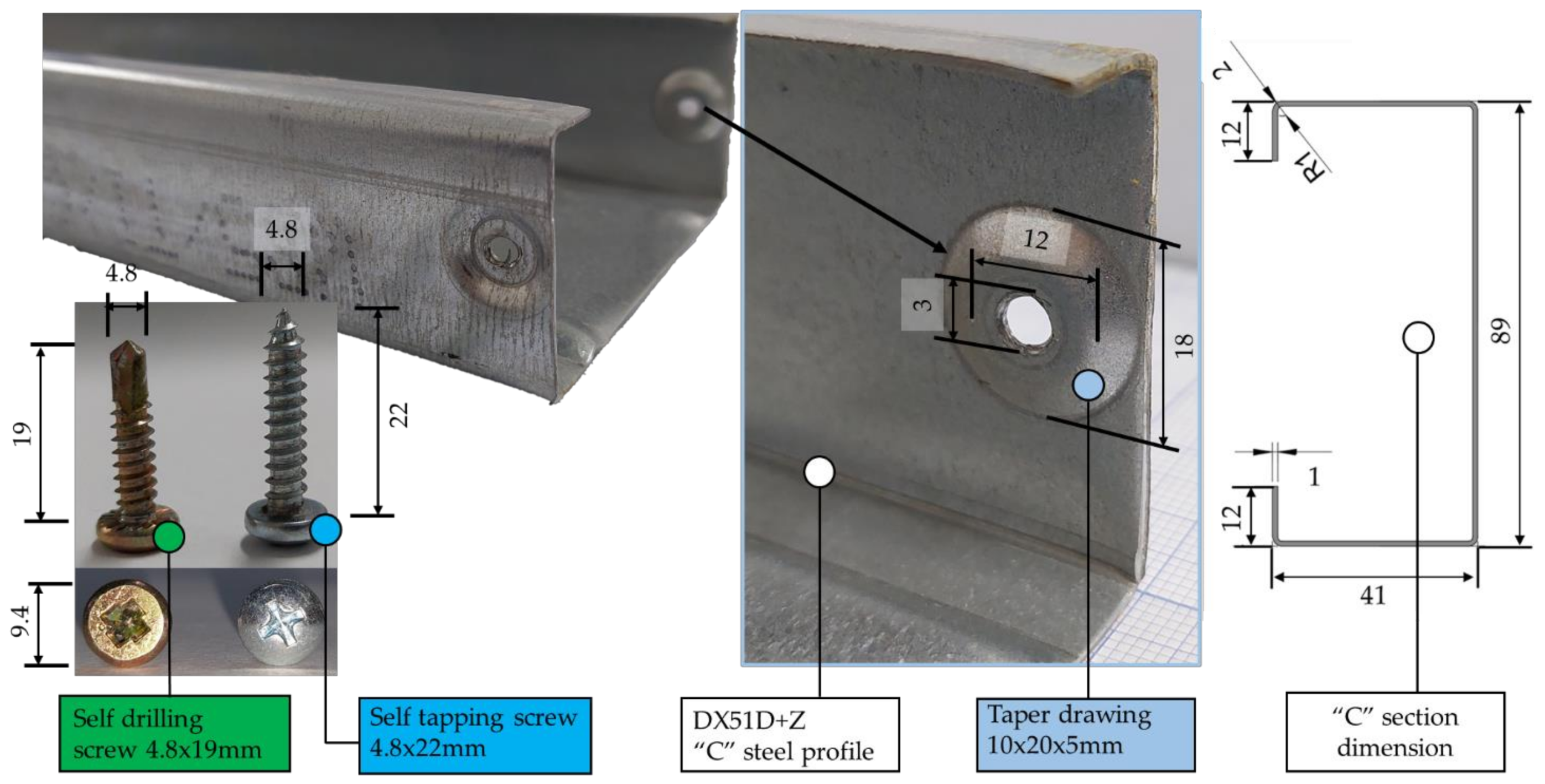
2. Materials and Methods
3. Experimental Results
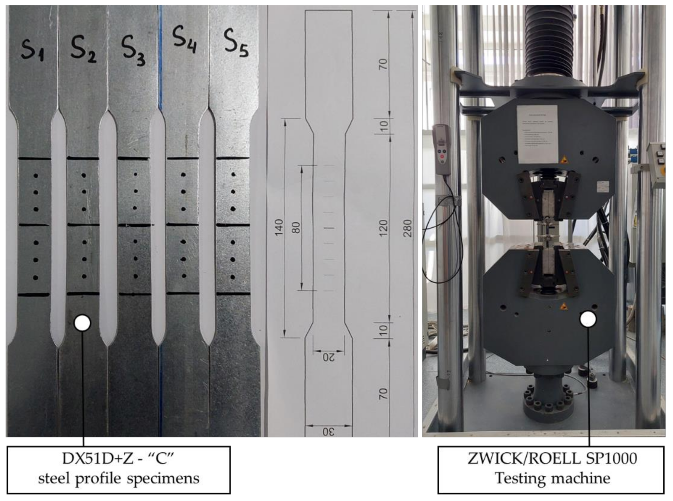
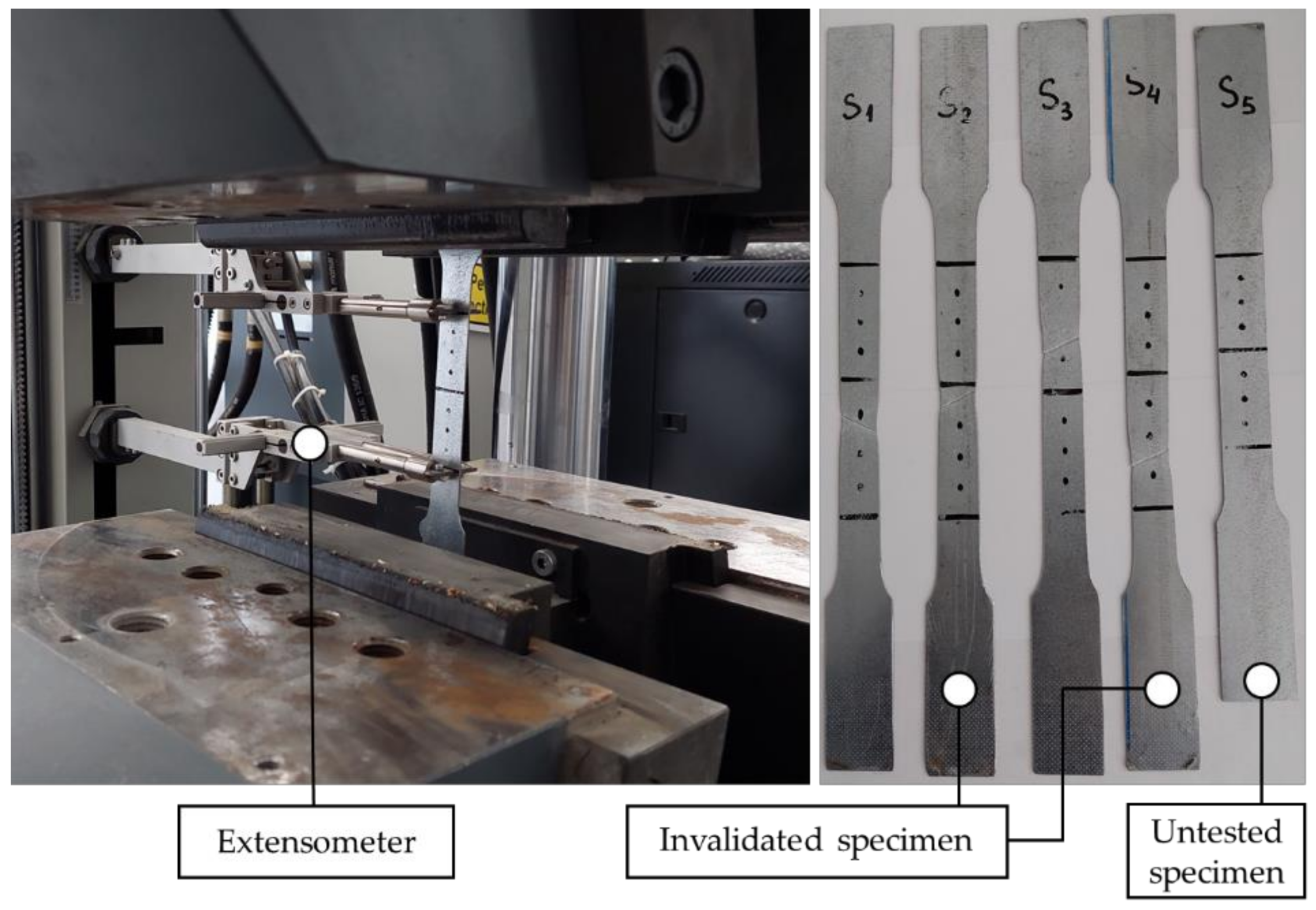
3.1. Sheet DX51D+Z Results
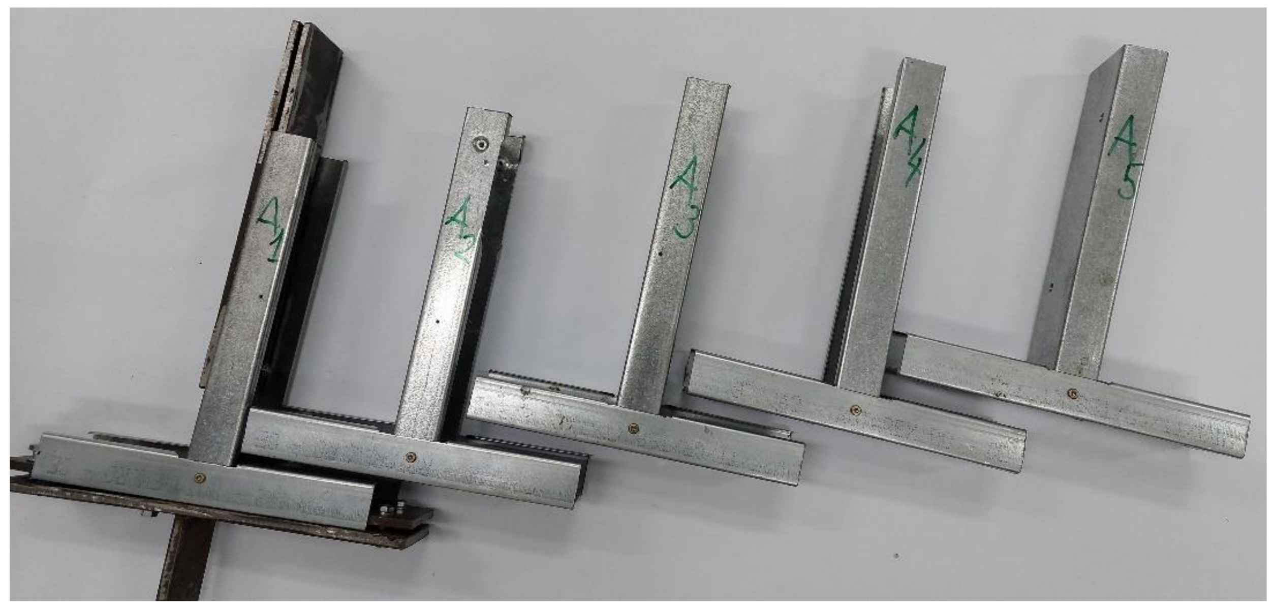
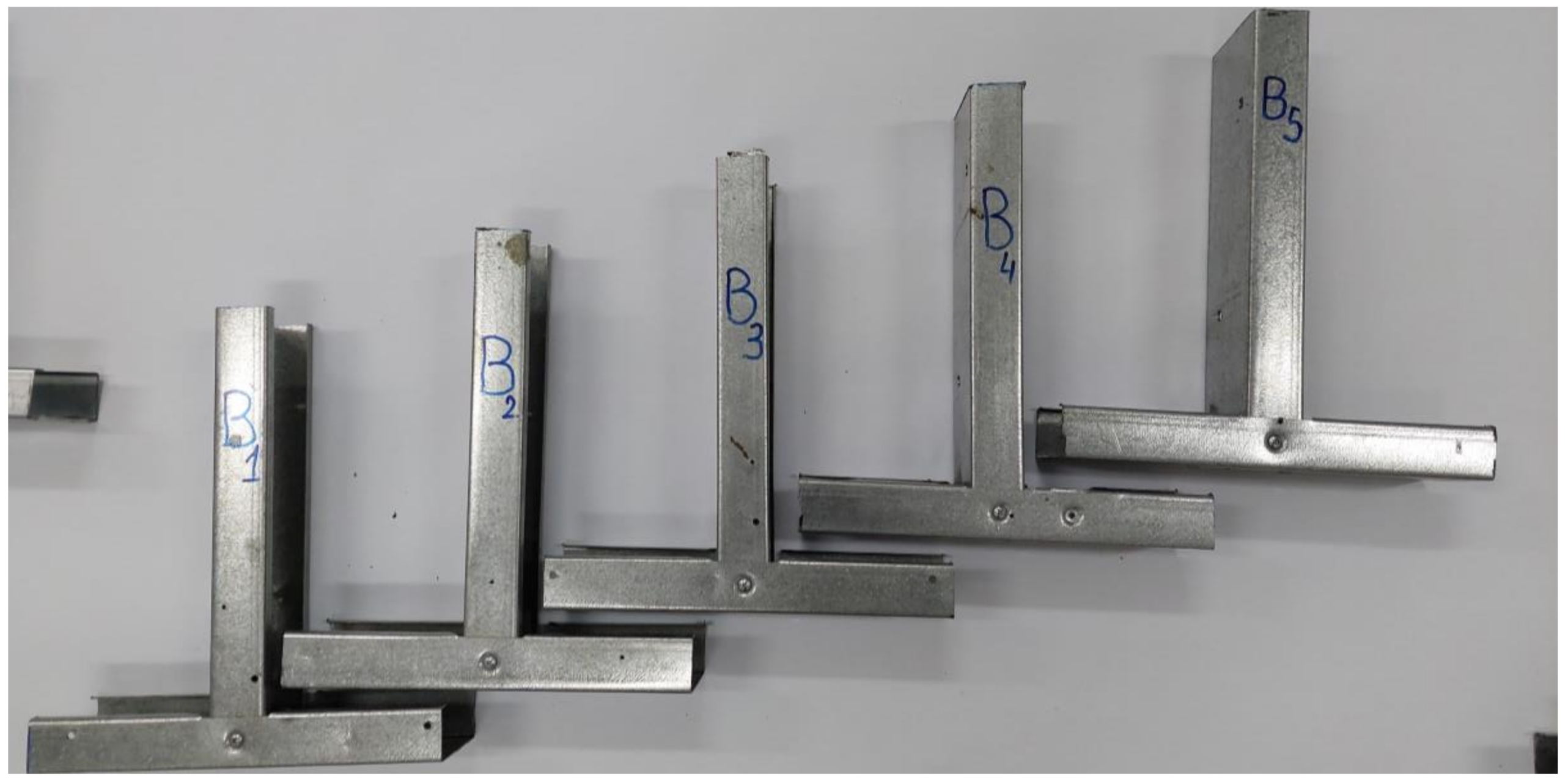
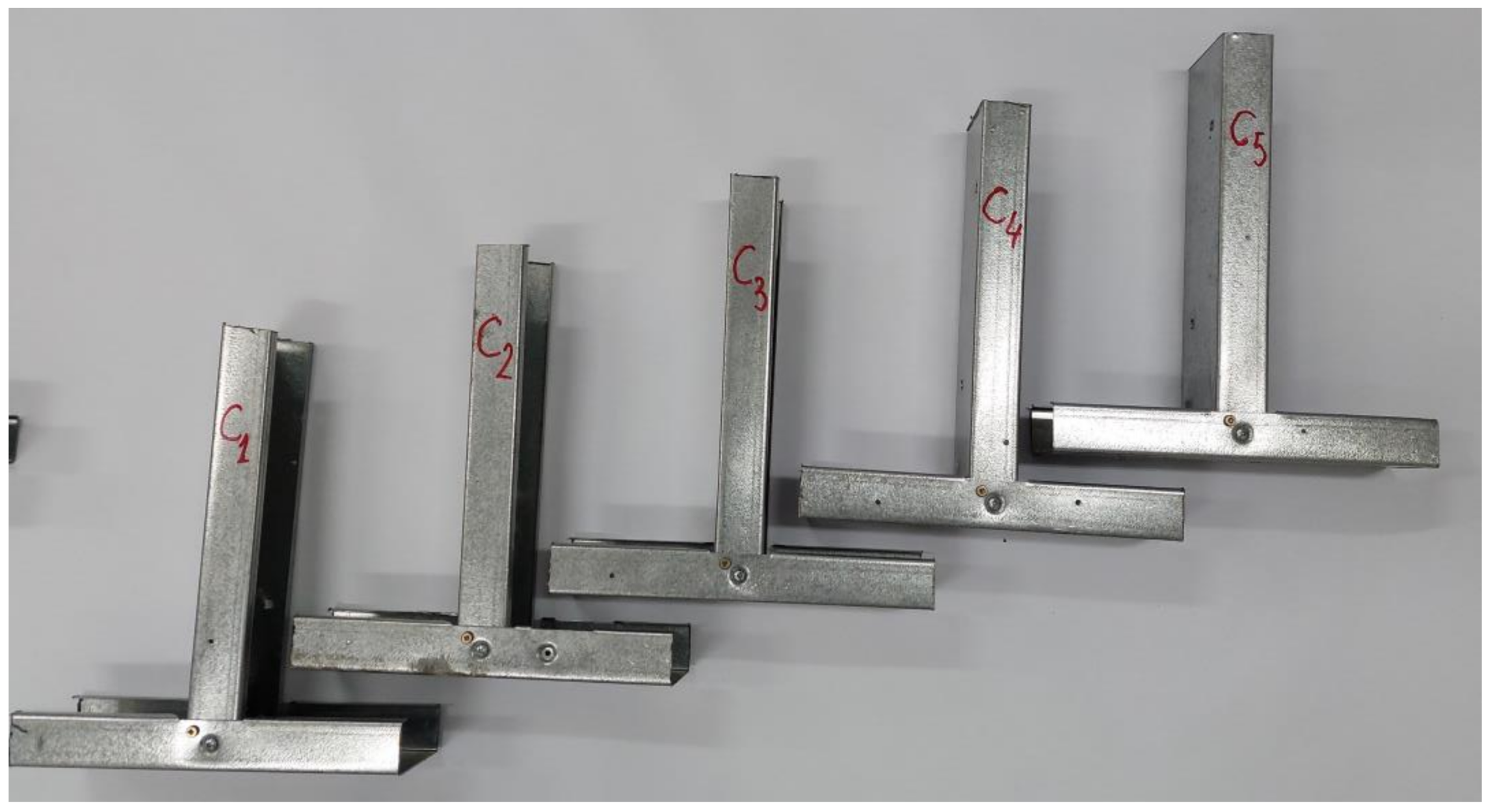
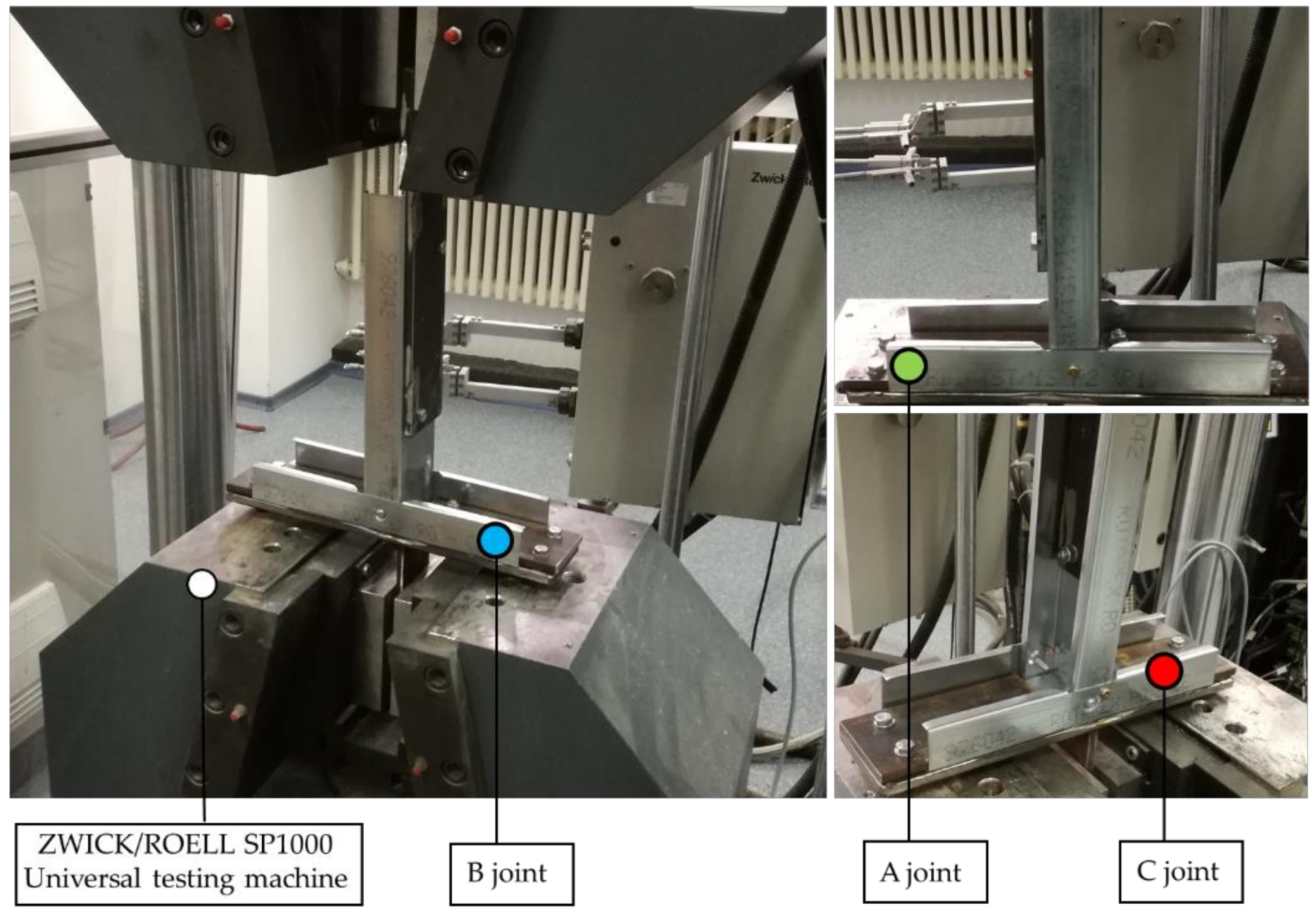
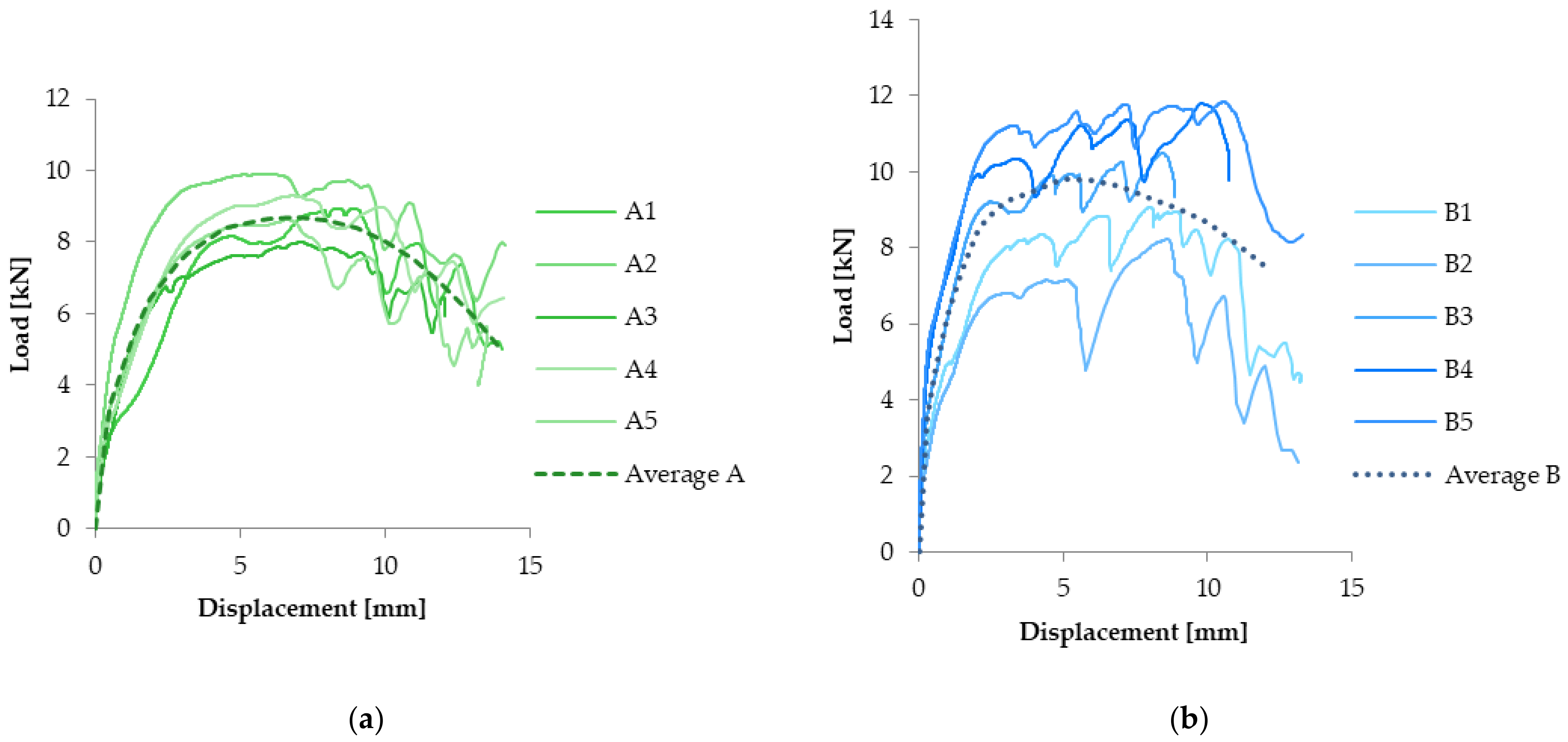
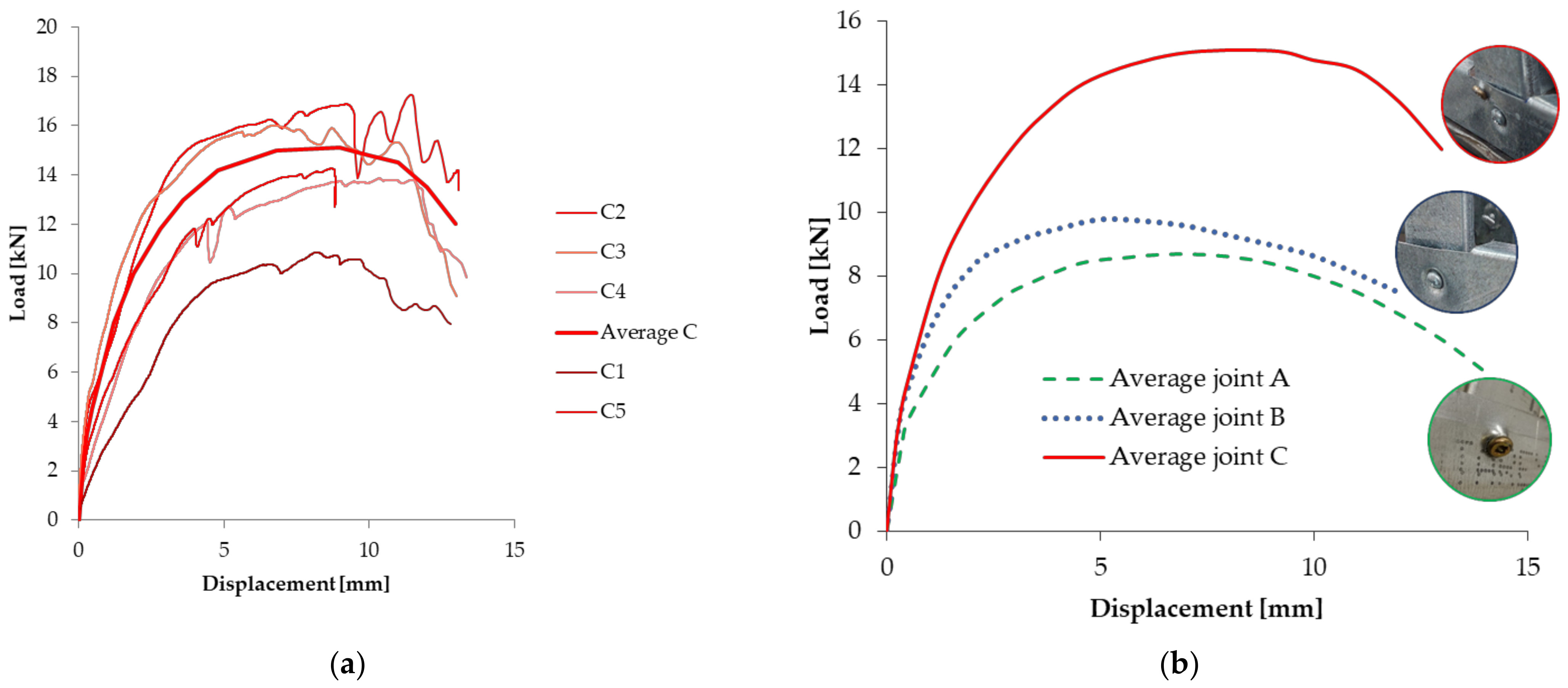
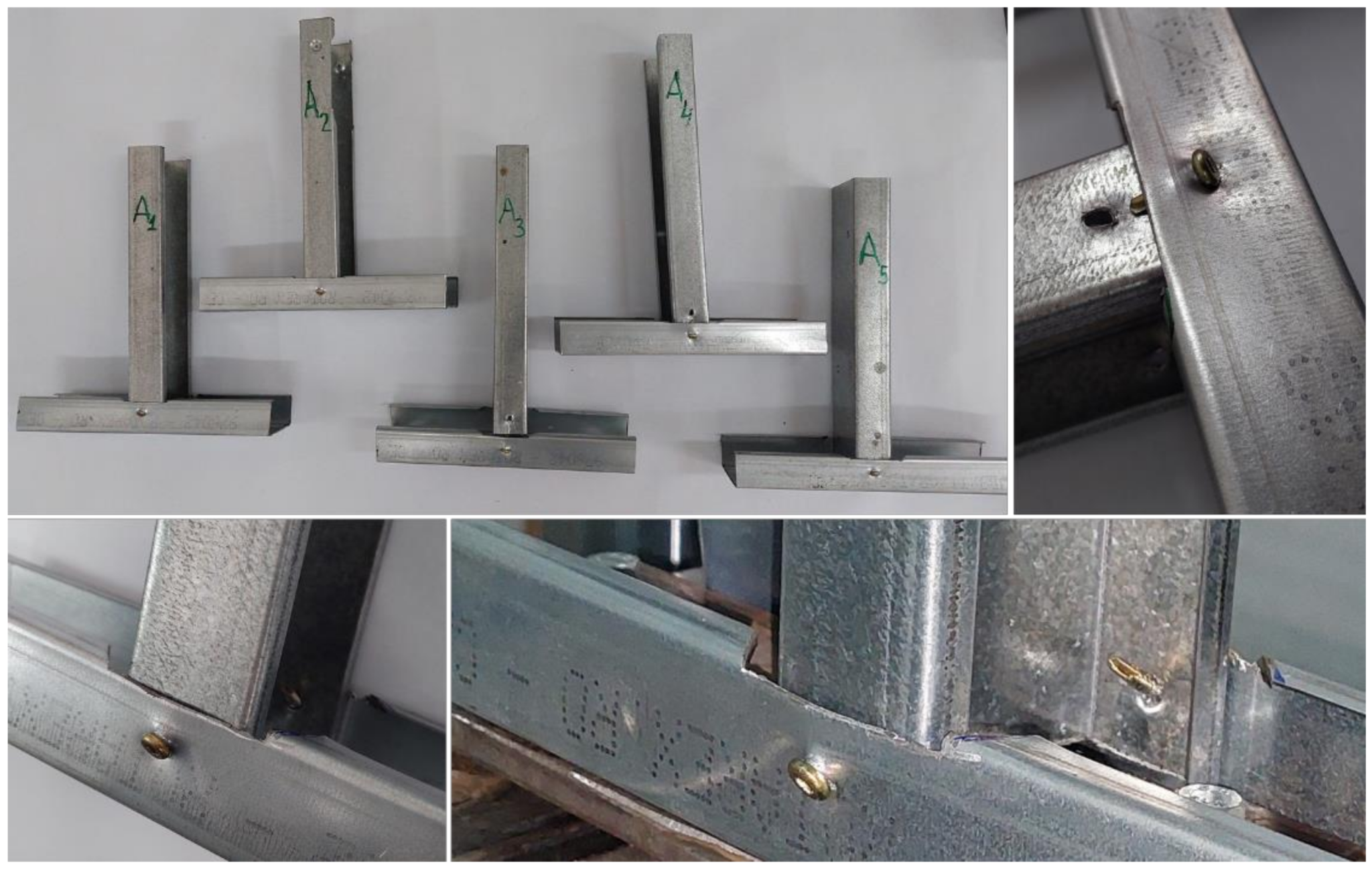
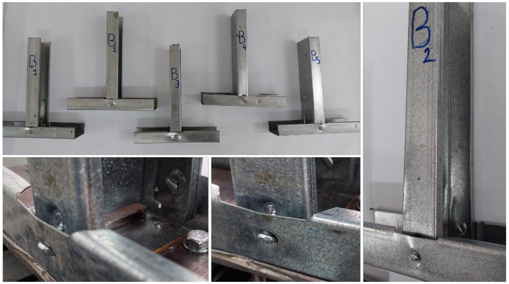
3.2. Joint Results
4. Finite Element Modelling
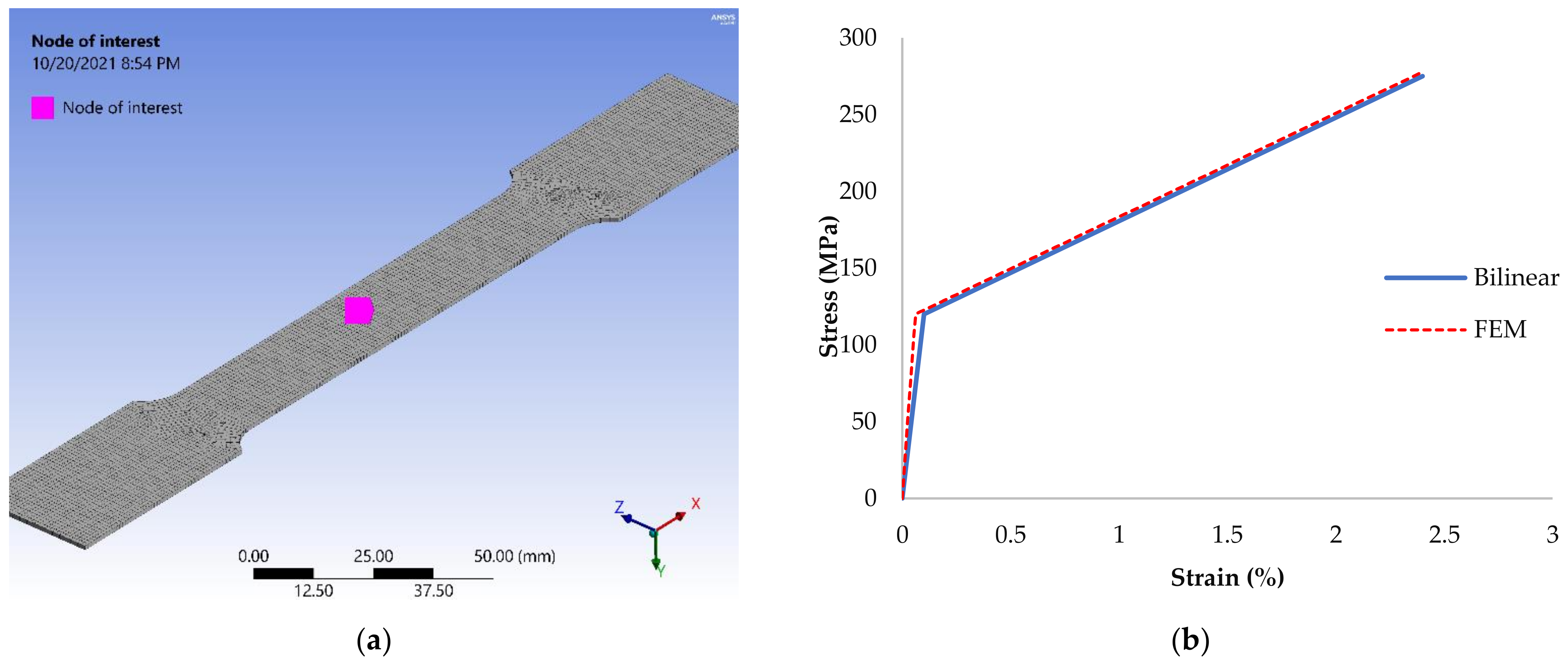
4.1. Nonlinear Analysis of the DX51D+Z Sheet Tensile Specimen
- Problem dimensionality: 3-d;
- Degrees of freedom: ux, uy, uz;
- Analysis type: static (steady-state);
- Offset temperature from absolute zero: 273.15;
- Nonlinear geometric effects: on;
- Equation solver option: sparse;
- Plastic material properties included: yes;
- Newton-Raphson option: program chosen;
- Globally assembled matrix: symmetric.
4.2. Results on Tensile Simulation Test
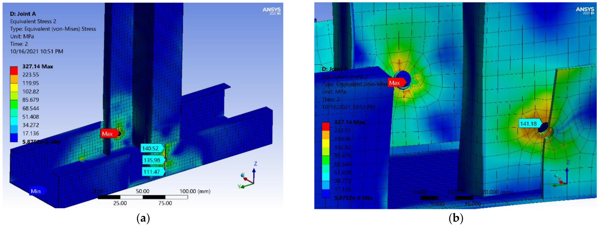
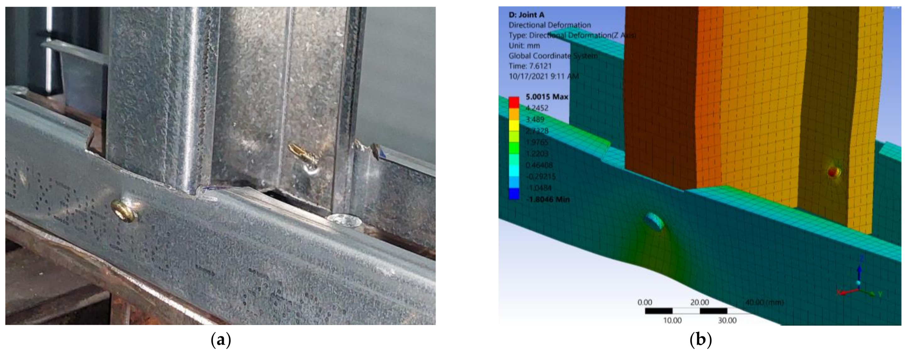
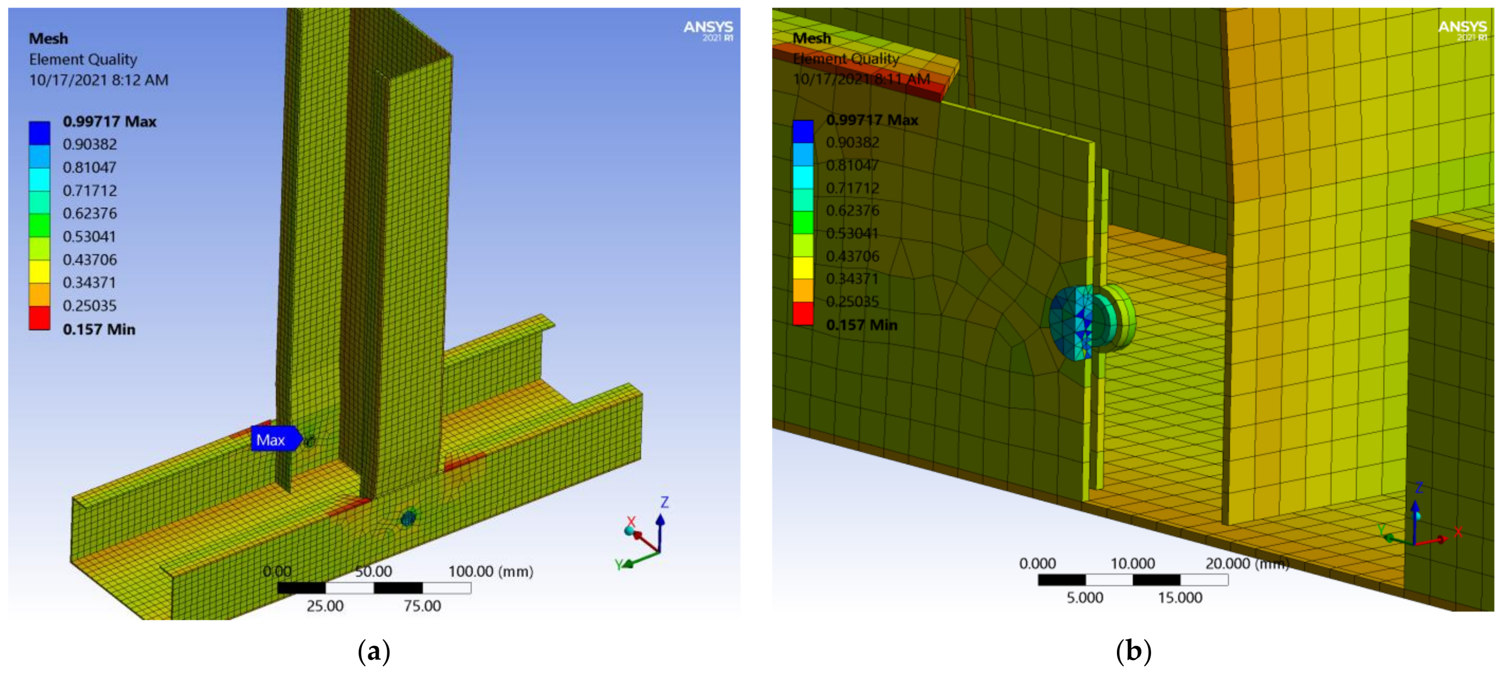
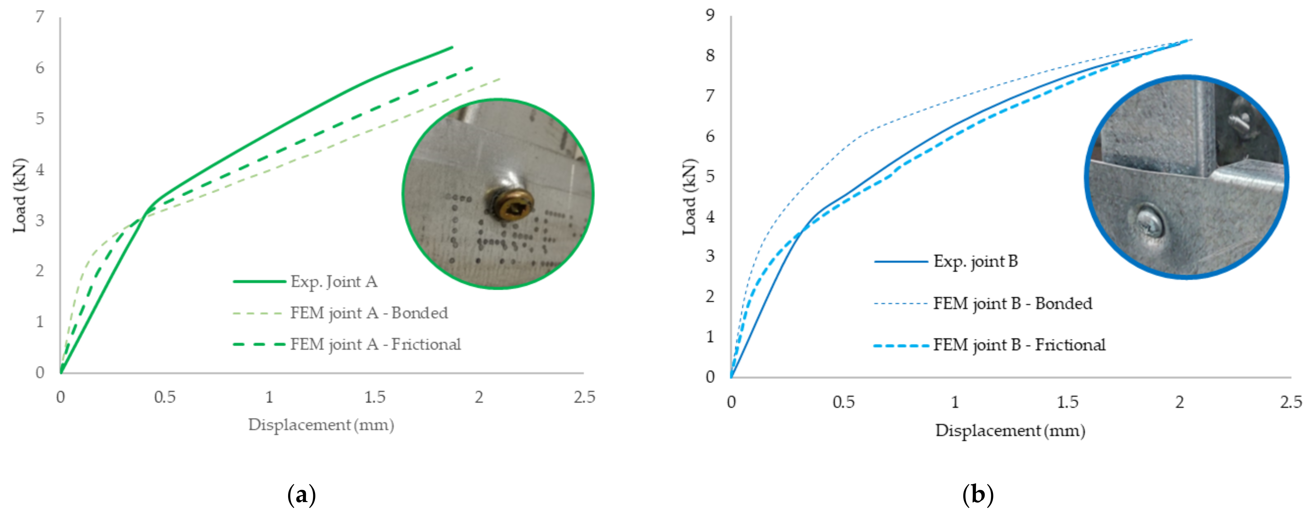
4.3. Joint A Modelling and Results
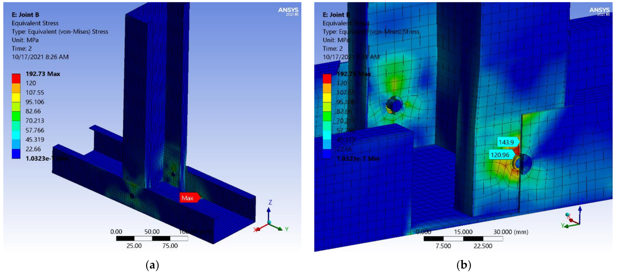
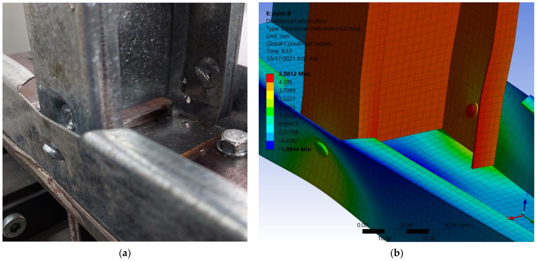
4.4. Joint B Modelling and Results
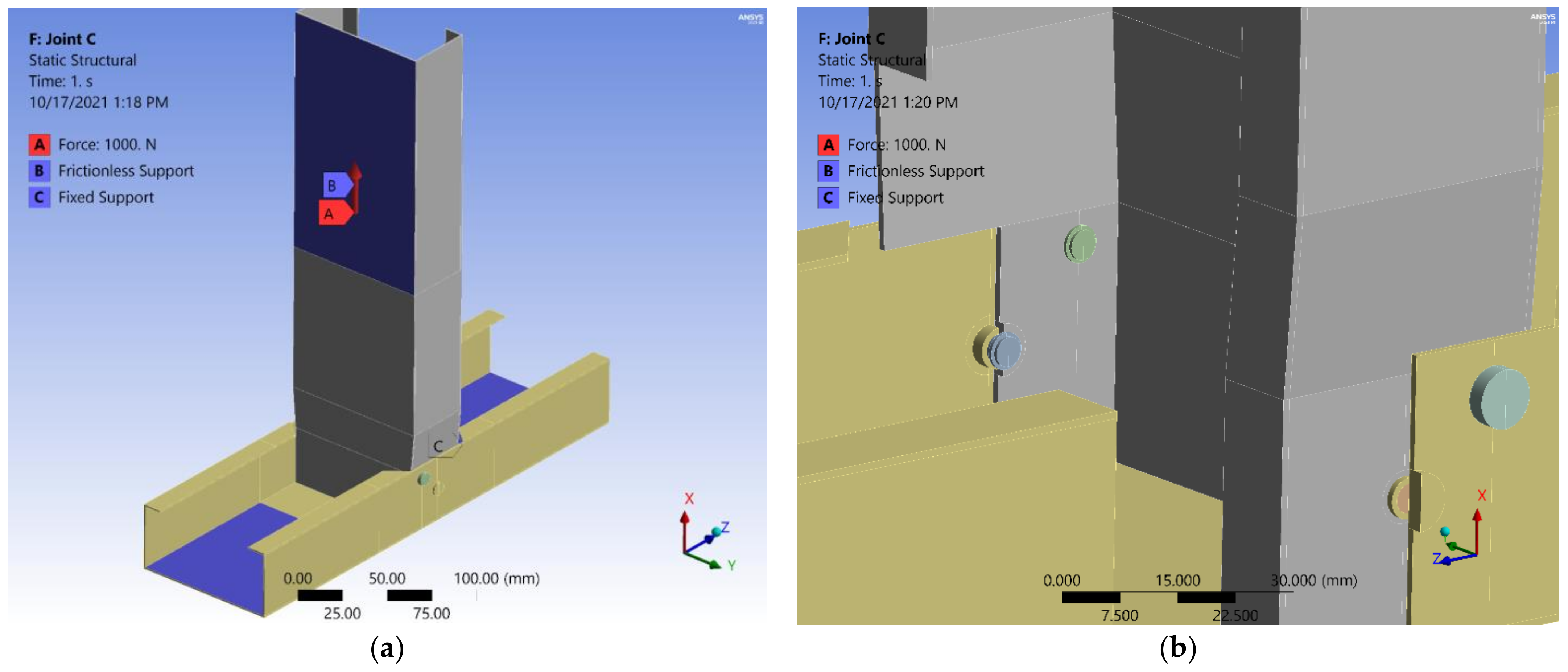
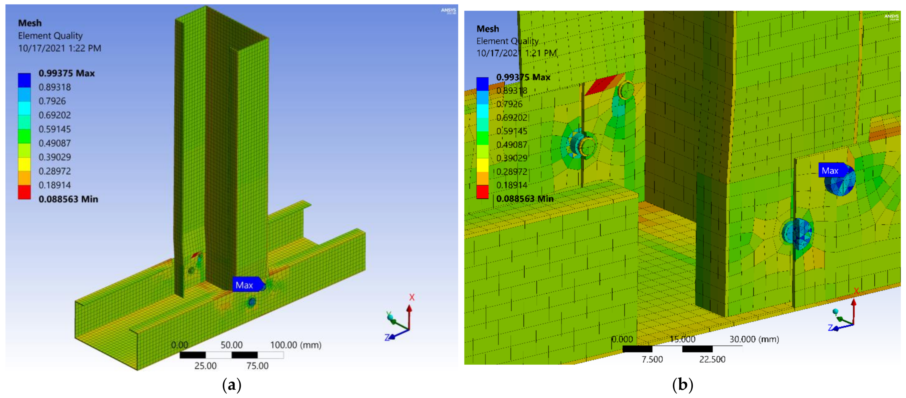
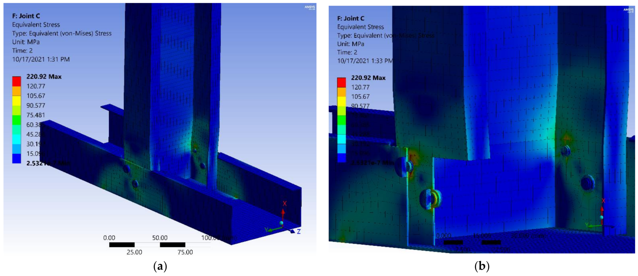
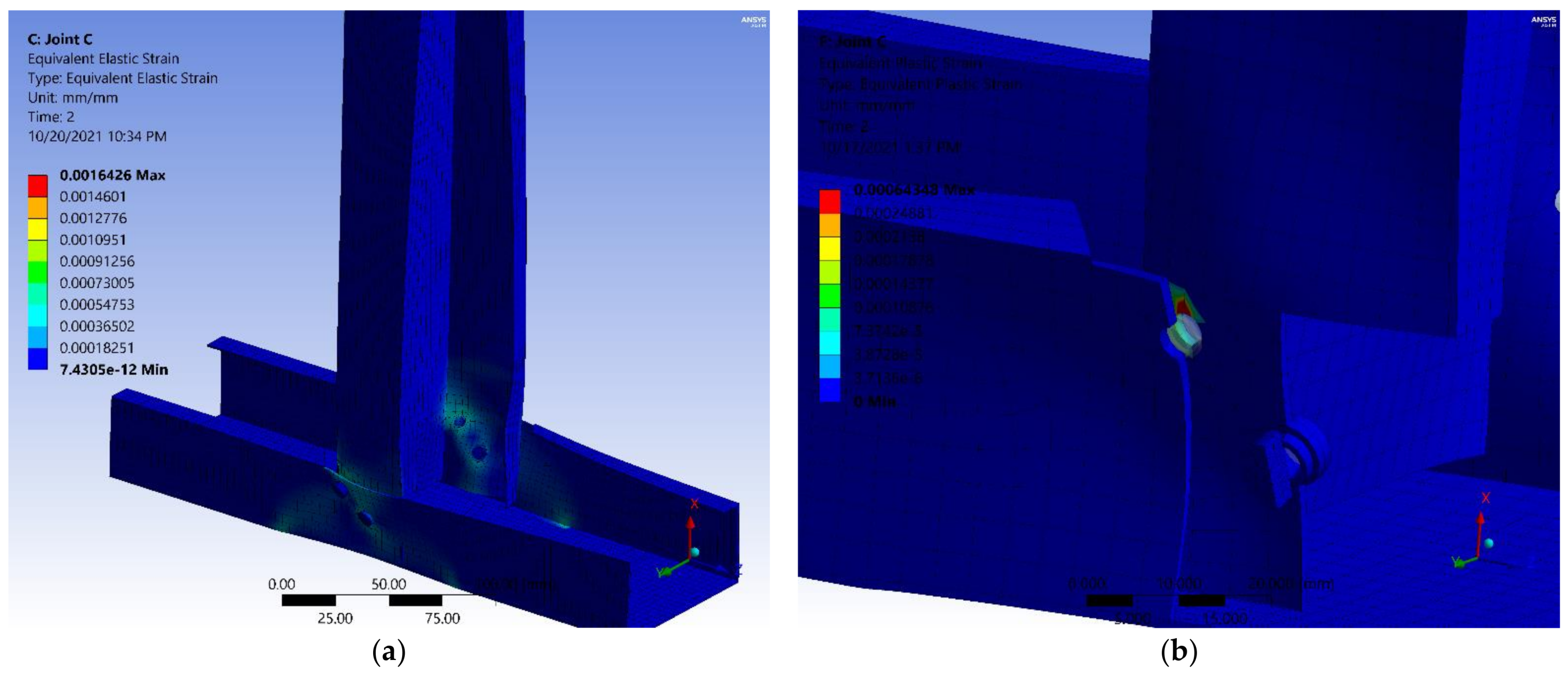
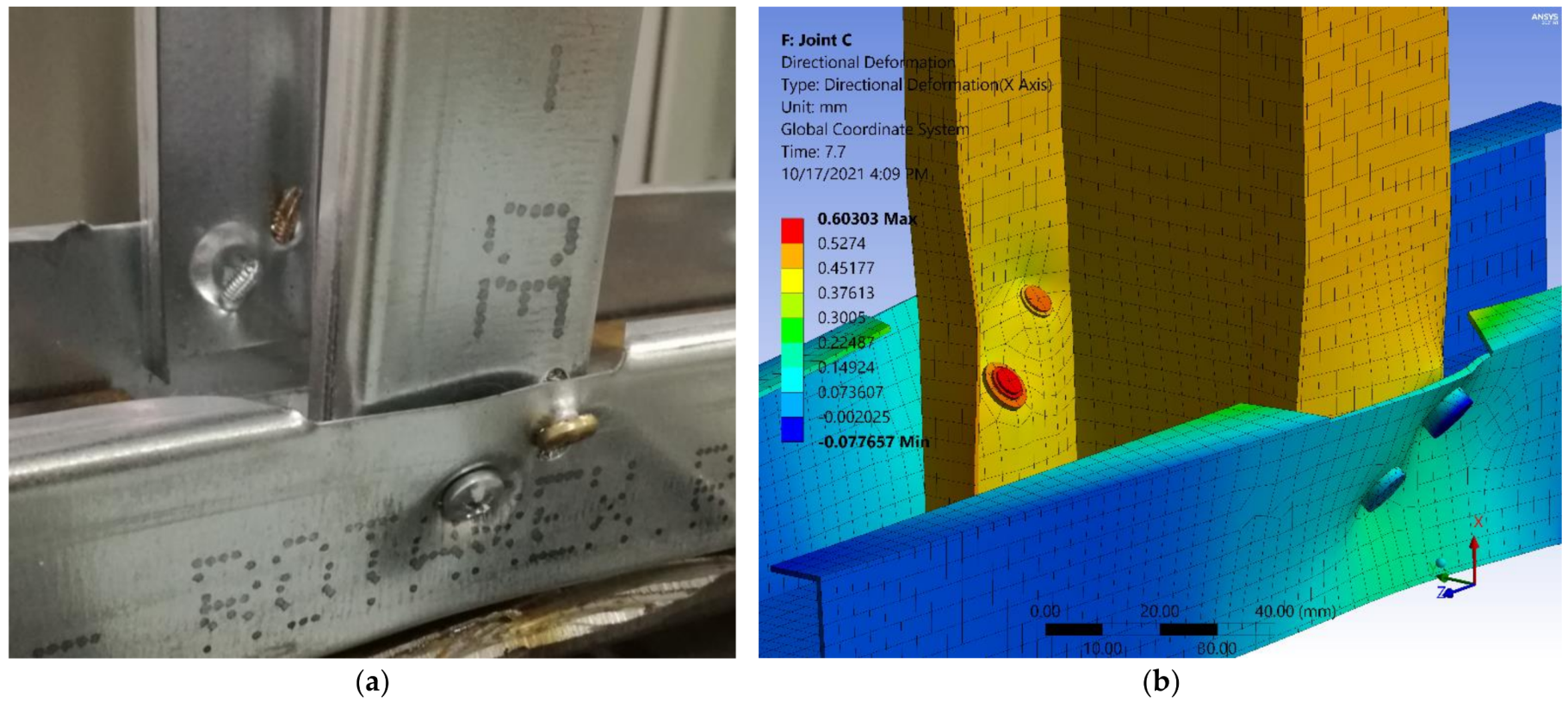
4.5. Joint C Modelling and Results
4.6. Design Resistance of Joint A, According to EN 1993-1-3
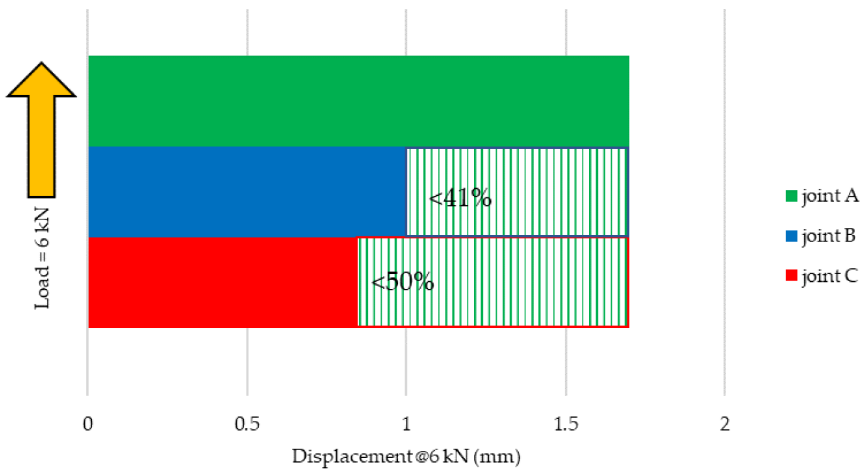
5. Discussion
6. Conclusions
Supplementary Materials
Author Contributions
Funding
Institutional Review Board Statement
Informed Consent Statement
Data Availability Statement
Acknowledgments
Conflicts of Interest
References
- Specification for the Design of Light Gage Steel Structural Members; American Iron and Steel Institute (AISI) Specifications, Standards, Manuals and Research Reports (1946–present); American Iron and Steel Institute: Washington, DC, USA, April 1946.
- EN 1993-1-3:2006. Eurocode 3: Design of Steel Structures—Part 1–3: General Rules-Supplementary Rules for Cold-Formed Members and Sheeting, 2007 [ECCS]. Available online: https://www.phd.eng.br/wp-content/uploads/2015/12/en.1993.1.3.2006.pdf (accessed on 19 October 2021).
- Landolfo, R. EUROCODES Background and Applications Cold-Formed (CF) Structures. Available online: https://eurocodes.jrc.ec.europa.eu/doc/WS2008/EN1999_8_Landolfo.pdf (accessed on 19 October 2021).
- Yu, W. Cold-Formed Steel Design; Wiley: Hoboken, NJ, USA, 2000; ISBN 0471-348-090. [Google Scholar]
- Blandford, G.E.; Louis, S. Current Research on Cold-Formed Steel Structures; International Specialty Conference on Cold-Formed Steel Structures. 1990. Available online: https://scholarsmine.mst.edu/isccss/10iccfss/10iccfss-session7/3 (accessed on 19 October 2021).
- Ungureanu, V.; Both, I.; Burcă, M.; Nguyen, T.H.; Grosan, M.; Dubină, D. Experimental Investigations on Spot Welded Built-Up Cold-Formed Steel Beams. Bull. Polytech. Inst. Jassy Construction. Archit. Sect. 2018, 64, 19–30. [Google Scholar] [CrossRef]
- Roşca, O.V. Experimental Tests of Thin-Walled Steel Roof Profiles. Bull. Polytech. Inst. Jassy Construction. Archit. Sect. 2011, LVII, 85–96. [Google Scholar]
- Ţăranu, G.; Budescu, M. 35 m Large Opening Roof Structural System Made of Hot Rolled and Cold Formed Steel Profiles. Bull. Polytech. Inst. Jassy Construction. Archit. Sect. 2018, 64, 33–40. [Google Scholar]
- Galatanu, T.; Ciongradi, I.P.; Budescu, M.; Rosca, O.V. Experimental Studies of the Back-To-Back Connected Cold Formed Steel Profile Bolted Joints. Bull. Polytech. Inst. Jassy 2009, 55, 17–28. [Google Scholar]
- Sivapathasundaram, M.; Mahendran, M. Pull-out Capacity of Multiple Screw Fastener Connections in Cold-Formed Steel Roof Battens. J. Constr. Steel Res. 2018, 144, 40–52. [Google Scholar] [CrossRef]
- Huynh, M.T.; Pham, C.H.; Hancock, G.J. Experimental Behaviour and Modelling of Screwed Connections of High Strength Sheet Steels in Shear. Thin-Walled Struct. 2020, 146, 106357. [Google Scholar] [CrossRef]
- Huynh, M.T.; Pham, C.H.; Hancock, G.J. Design of Screwed Connections in Cold-Formed Steels in Shear. Thin-Walled Struct. 2020, 154, 106817. [Google Scholar] [CrossRef]
- Roy, K.; Lau, H.H.; Huon Ting, T.C.; Masood, R.; Kumar, A.; Lim, J.B.P. Experiments and Finite Element Modelling of Screw Pattern of Self-Drilling Screw Connections for High Strength Cold-Formed Steel. Thin-Walled Struct. 2019, 145, 106393. [Google Scholar] [CrossRef]
- Wu, H.; Chao, S.; Li, Y.; Sang, L. Experimental Investigation of Strengthened Screw Connection and Application in CFS Shear Walls. J. Constr. Steel Res. 2020, 168, 105870. [Google Scholar] [CrossRef]
- Quan, G.; Ye, J.; Li, W. Computational Modelling of Cold-Formed Steel Lap Joints with Screw Fasteners. Structures 2021, 33, 230–245. [Google Scholar] [CrossRef]
- Nithyadharan, M.; Kalyanaraman, V. A New Screw Connection Model and FEA of CFS Shear Wall Panels. J. Constr. Steel Res. 2021, 176, 106430. [Google Scholar] [CrossRef]
- Feng, R.Q.; Cai, Q.; Ma, Y.; Yan, G. rong Shear Analysis of Self-Drilling Screw Connections of CFS Walls with Steel Sheathing. J. Constr. Steel Res. 2020, 167, 105842. [Google Scholar] [CrossRef]
- Henriques, J.; Rosa, N.; Gervasio, H.; Santos, P.; da Silva, L.S. Structural Performance of Light Steel Framing Panels Using Screw Connections Subjected to Lateral Loading. Thin-Walled Struct. 2017, 121, 67–88. [Google Scholar] [CrossRef]
- Xie, Z.; Yan, W.; Yu, C.; Mu, T.; Song, L. Experimental Investigation of Cold-Formed Steel Shear Walls with Self-Piercing Riveted Connections. Thin-Walled Struct. 2018, 131, 1–15. [Google Scholar] [CrossRef]
- Xie, Z.; Yan, W.; Yu, C.; Mu, T.; Song, L. Improved Shear Strength Design of Cold-Formed Steel Connection with Single Self-Piercing Rivet. Thin-Walled Struct. 2018, 131, 708–717. [Google Scholar] [CrossRef]
- Song, L.; Yan, W.; Zhang, X.; Yu, C.; Xie, Z. Feasibility Research on the Application of Self-Piercing Riveted Connection in Cold-Formed Steel Structures. J. Constr. Steel Res. 2020, 168, 105957. [Google Scholar] [CrossRef]
- Light Steel Structure Factory. Steel House Producer. Available online: https://www.rotarex.ro/en/ (accessed on 19 October 2021).
- Dubina, D.; Stratan, A.; Ciutina, A.; Fulop, L.; Nagy, Z. Strength, Stiffness and Ductility of Cold-Formed Steel Bolted Connections. Available online: https://scholar.google.com/scholar?cluster=10778266862457140001&hl=en&oi=scholarr (accessed on 19 October 2021).
- Dubina, D.; Fülöp, L.A.; Aldea, A.; Demetriu, S.; Nagy, Z. Seismic Performance of Cold-Formed Steel Framed Houses. In Proceedings of the 5th International Conference on Behaviour of Steel Structures in Seismic Areas (STESSA), Yokohama, Japan, 14–17 August 2006; pp. 429–435. [Google Scholar]
- Dubina, D.; Fülöp, L.; Ungureanu, V.; Szabo, I.; Nagy, Z. Cold-Formed Steel Structures for Residential and Non-Residential Buildings. In Proceedings of the 9th International Conference on Metal Structures, Timisoara, Romania, 19–22 October 2000; pp. 308–317. [Google Scholar]
- Thirunavukkarasu, K.; Kanthasamy, E.; Gatheeshgar, P.; Poologanathan, K.; Rajanayagam, H.; Suntharalingam, T.; Dissanayake, M. Sustainable Performance of a Modular Building System Made of Built-Up Cold-Formed Steel Beams. Buildings 2021, 11, 460. [Google Scholar] [CrossRef]
- Taranu, G.; Budescu, M.; Olteanu, I.; Toma, I.-O.; Venghiac, M.; Stratulat, M. Sisteme Structurale de Rezistentă Cu Profile Din Tabla Subtire Indoite La Rece Tip ROTAREX. Available online: http://www.aicps.ro/revista/aicps-review-1-2-2018/content#page/n0/mode/2up (accessed on 16 October 2021).
- International Organization for Standardization ISO 6892-1:2019(En), Metallic Materials—Tensile Testing—Part 1: Method of Test at Room Temperature. Available online: https://www.iso.org/obp/ui/#iso:std:iso:6892:-1:ed-3:v1:en (accessed on 5 October 2021).
- Grabber Flat Pan Head Driller 4.8 × 19 mm Heavy Gauge Metal Framing–Self Drilling Screws Technical Data. Available online: https://www.grabberman.com/Media/TechnicalData/512.pdf (accessed on 2 October 2021).
- INDEX Self Tapping Screw 4.8 × 22 mm DIN 7981 Technical Data Sheet. Available online: https://www.indexfix.com/docs/ft-ros-en.pdf (accessed on 2 October 2021).
- Flodr, J.; Kałduński, P.; Krejsa, M.; Pařenica, P. Innovative Connection of Steel Profiles, Experimental Verification and Application. Procedia Eng. 2017, 190, 215–222. [Google Scholar] [CrossRef]
- Petrik, A.; Aroch, R. Usage of True Stress-Strain Curve for FE Simulation and the Influencing Parameters. In IOP Conference Series: Materials Science and Engineering; Institute of Physics Publishing: Bristol, UK, 2019; Volume 566, p. 012025. [Google Scholar]
- Yao, D.; Cai, L.; Bao, C. A New Approach on Necking Constitutive Relationships of Ductile Materials at Elevated Temperatures. Chin. J. Aeronaut. 2016, 29, 1626–1634. [Google Scholar] [CrossRef] [Green Version]


| Component | Type | Elastic Modulus (GPa) | Tensile Strength (MPa) | Shear Strength (MPa) |
|---|---|---|---|---|
Profile steel sheet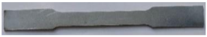 | DX51D+Z | 210 | 250 | - |
Self-drilling screw—SDR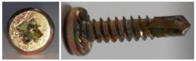 | 4.8 × 19 mm [29] | 210 | 1531 | 1313 |
Self-tapping screw—STR | 4.8 × 22 mm [30] | 210 | 1000 | 500 |
| Basic Data | ||
| Nominal diameter of the screw | (3) | |
| Total number of screws | (4) | |
| End and edge distance for screw | (5) | |
| The dimensions of the stud cross-section: | ||
| Total height | (6) | |
| Total width of flange | (7) | |
| Total width of edge fold | (8) | |
| Nominal thickness | (9) | |
| Steel core thickness | (10) | |
| Gross area of the studied cross-section | (11) | |
| The dimensions of the rail cross-section: | ||
| Total height | (12) | |
| Total width of flange | (13) | |
| Nominal thickness | (14) | |
| Steel core thickness | (15) | |
| The materials properties are: | ||
| Basic yield strength | (16) | |
| Ultimate strength | (17) | |
| Modulus of elasticity | (18) | |
| Poisson’s ratio | (19) | |
| Shear modulus | (20) | |
| Partial factor | (21) | |
| The design force on the connection | (22) | |
| The design shear force per screw in the ultimate limit state is: | (23) | |
| Check the range of validity for design resistance formulas | ||
| The following conditions should be satisfied: | ||
| (24) | ||
| OK | (25) | |
| OK | (26) | |
| OK | (27) | |
| Resistance check for self-tapping screws loaded in shear | ||
| Bearing resistance | (28) | |
| (29) | ||
| The bearing resistance of one screw is: | (30) | |
| Net-section resistance | (31) | |
| (32) | ||
| The net-section resistance is: | (33) | |
| Shear resistance | (34) | |
| (35) | ||
| The resistance of a fastener in shear may be verified using | ||
| (36) | ||
| (37) | ||
Publisher’s Note: MDPI stays neutral with regard to jurisdictional claims in published maps and institutional affiliations. |
© 2021 by the authors. Licensee MDPI, Basel, Switzerland. This article is an open access article distributed under the terms and conditions of the Creative Commons Attribution (CC BY) license (https://creativecommons.org/licenses/by/4.0/).
Share and Cite
Taranu, G.; Toma, I.-O. Experimental Investigation and Numerical Simulation of C-Shape Thin-Walled Steel Profile Joints. Buildings 2021, 11, 636. https://doi.org/10.3390/buildings11120636
Taranu G, Toma I-O. Experimental Investigation and Numerical Simulation of C-Shape Thin-Walled Steel Profile Joints. Buildings. 2021; 11(12):636. https://doi.org/10.3390/buildings11120636
Chicago/Turabian StyleTaranu, George, and Ionut-Ovidiu Toma. 2021. "Experimental Investigation and Numerical Simulation of C-Shape Thin-Walled Steel Profile Joints" Buildings 11, no. 12: 636. https://doi.org/10.3390/buildings11120636
APA StyleTaranu, G., & Toma, I.-O. (2021). Experimental Investigation and Numerical Simulation of C-Shape Thin-Walled Steel Profile Joints. Buildings, 11(12), 636. https://doi.org/10.3390/buildings11120636