Exploring the Influence of an Urban Water System on Housing Prices: Case Study of Zhengzhou


Abstract
1. Introduction
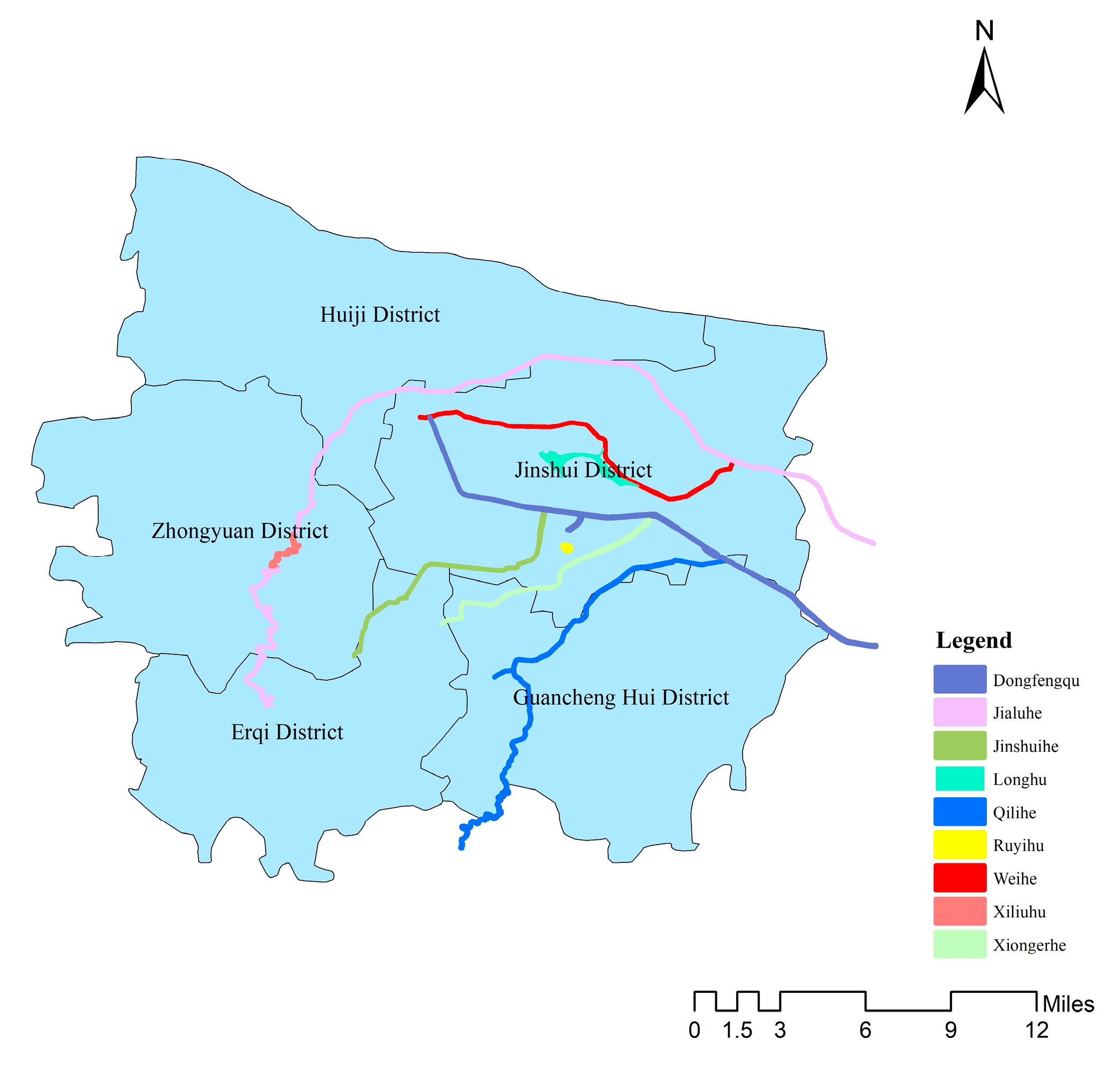
2. Research Area
3. Data and Method
3.1. Variable Setting
3.2. Data Collection and Processing
3.3. Model Specification
4. Research Results
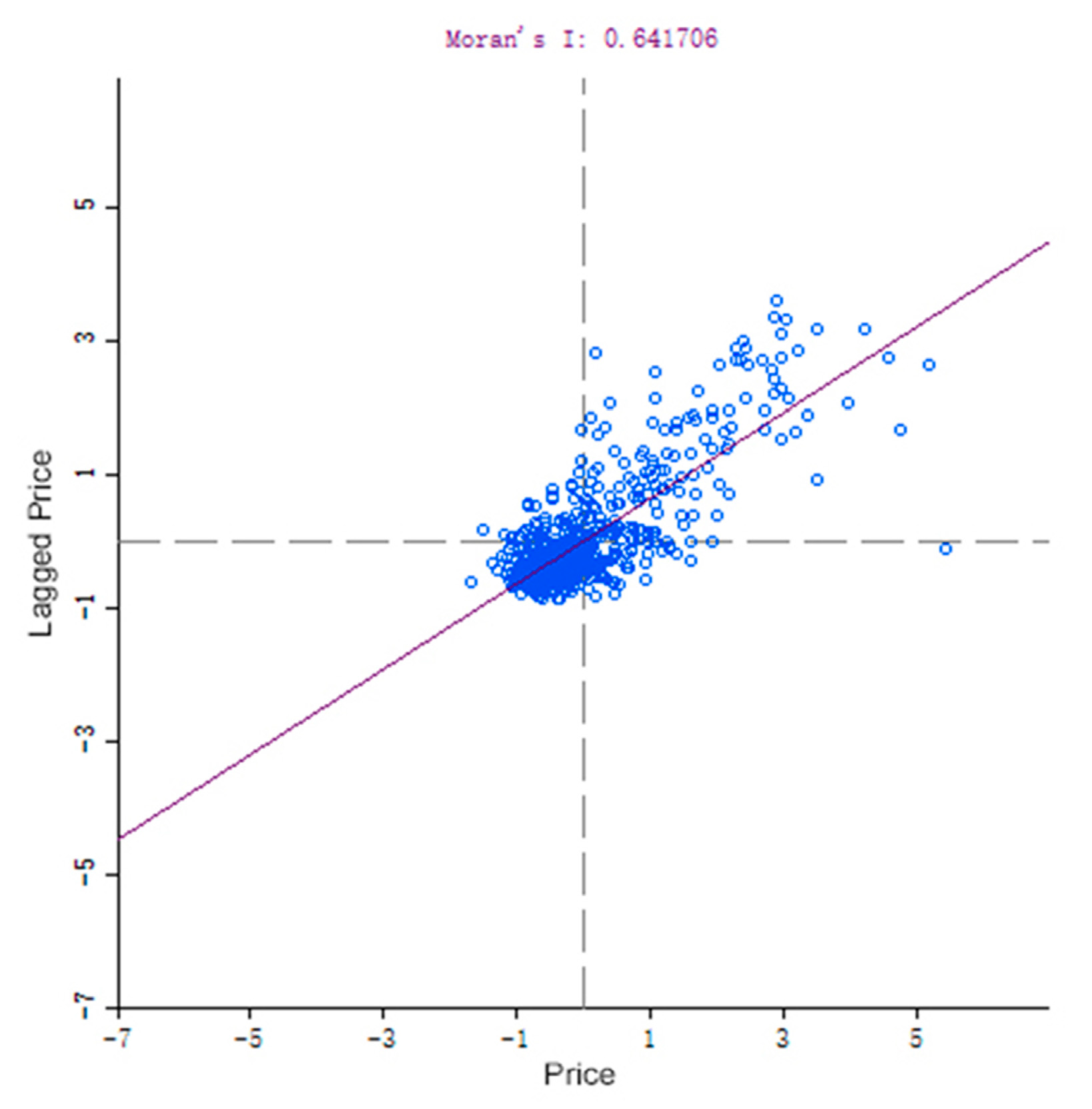
4.1. Results Analysis of Traditional Model
4.2. Result Analysis of Spatial Lag Model
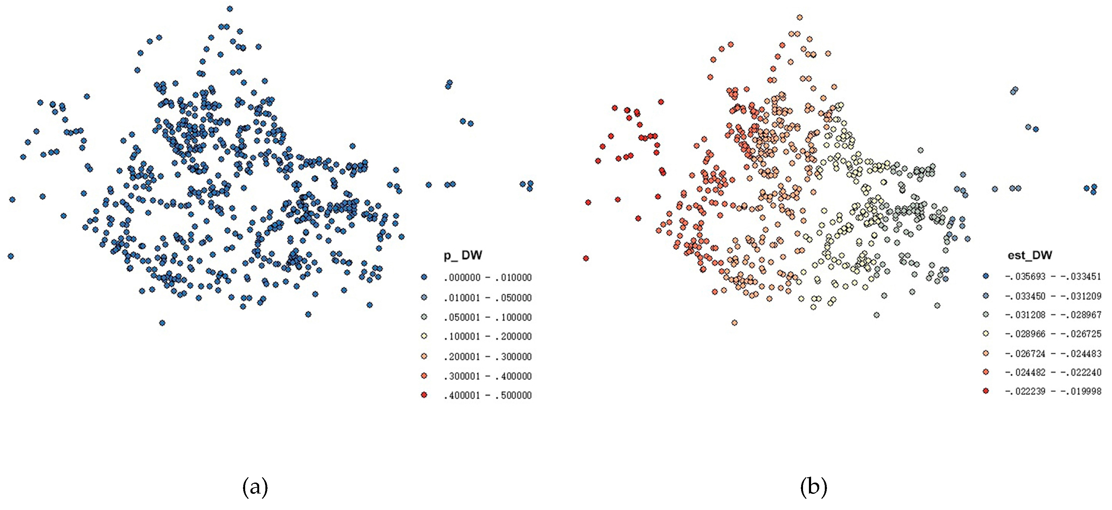
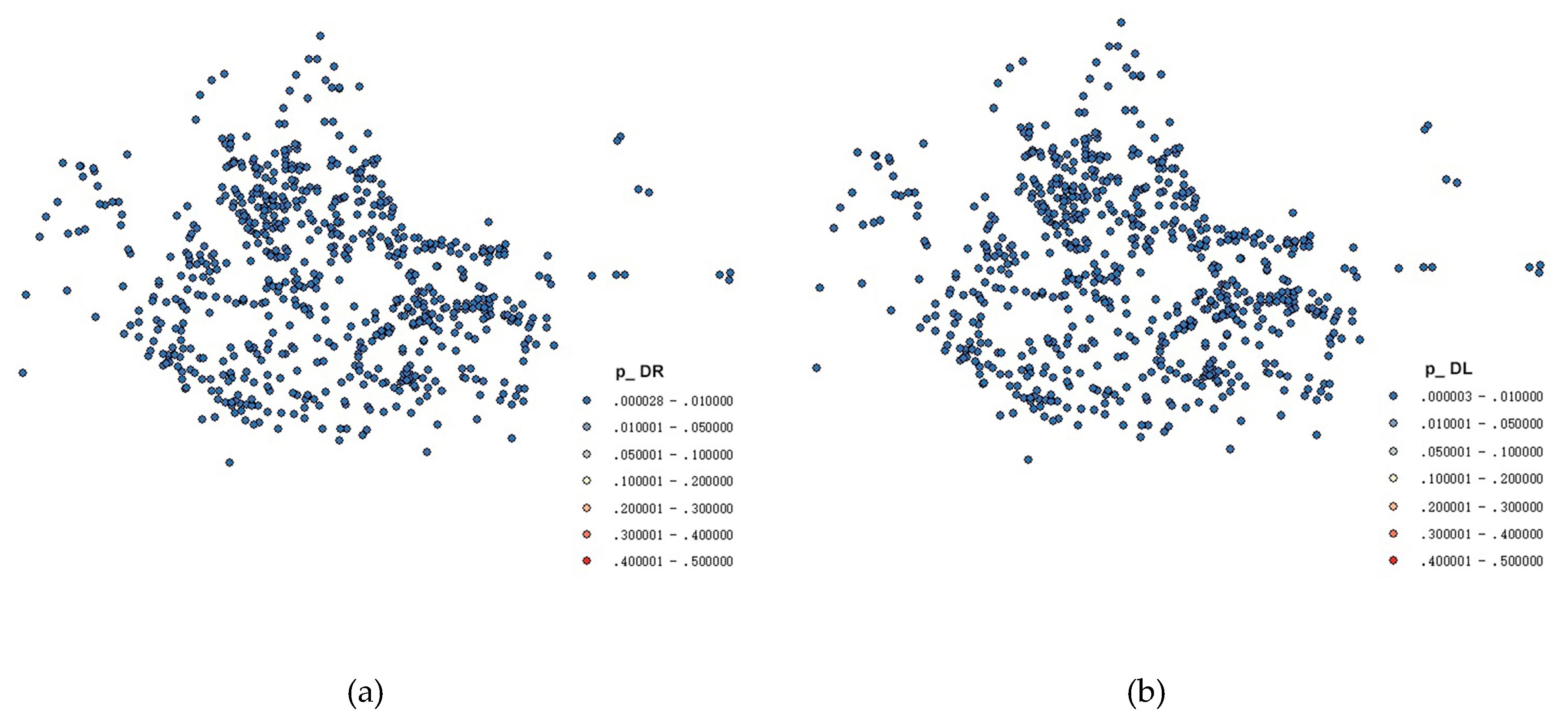
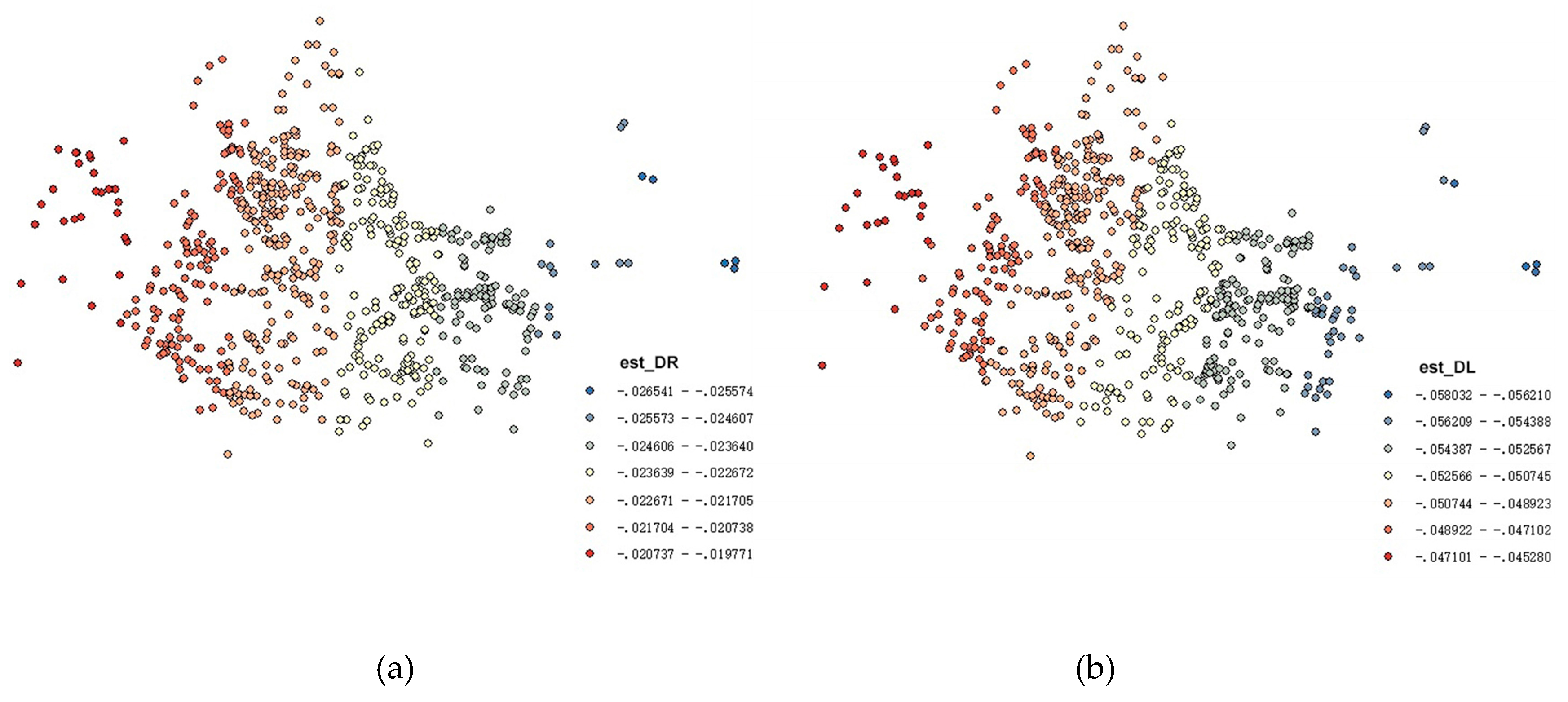
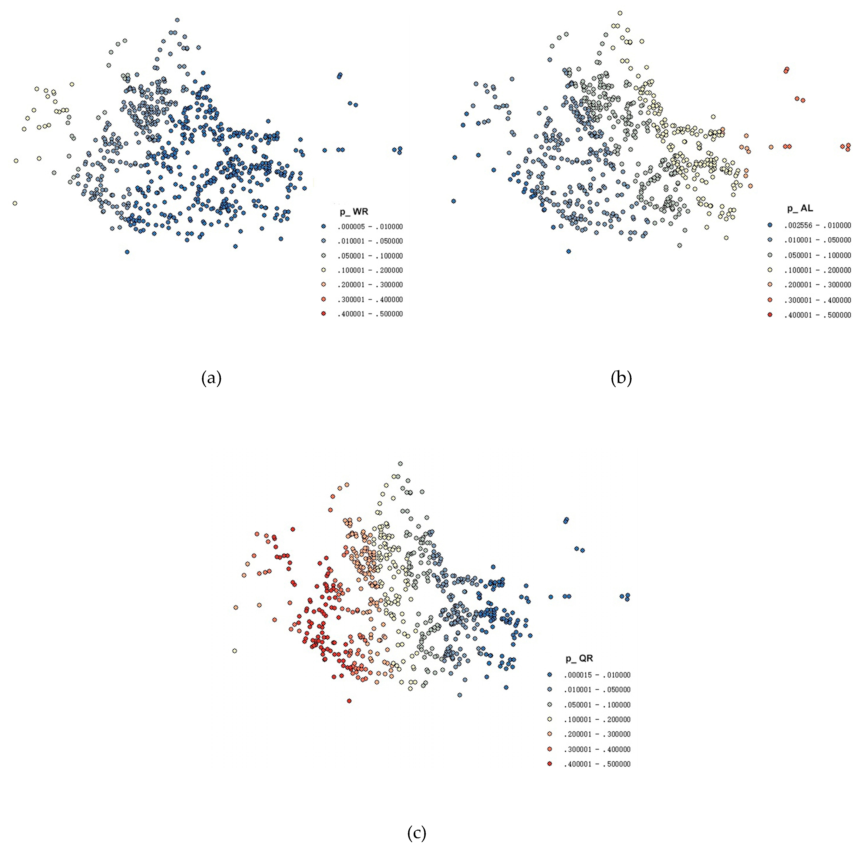
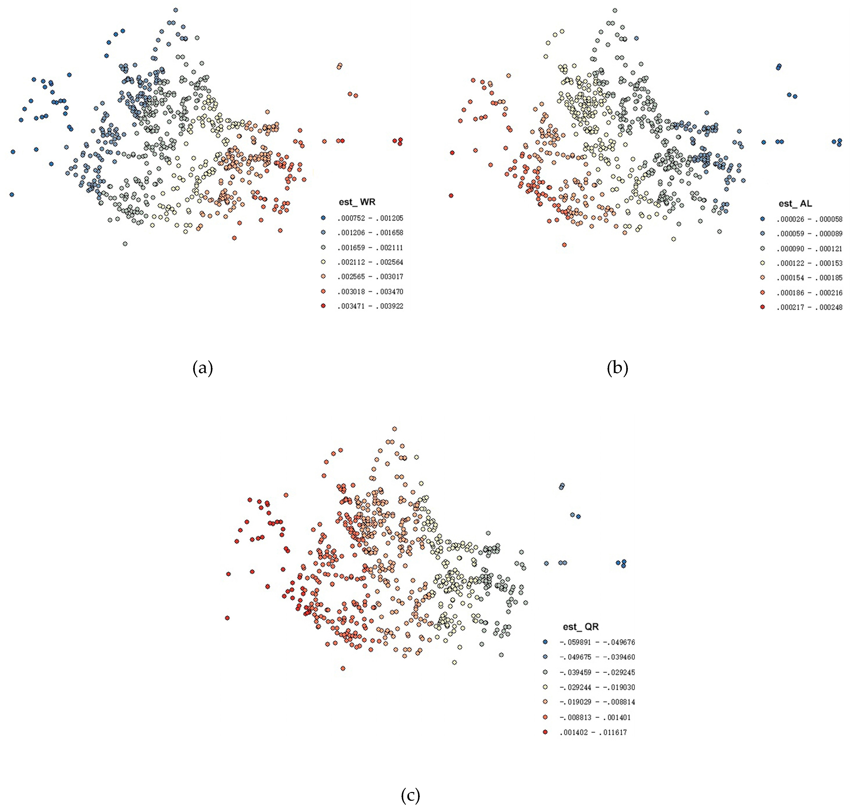
4.3. Results Analysis of GWR Model
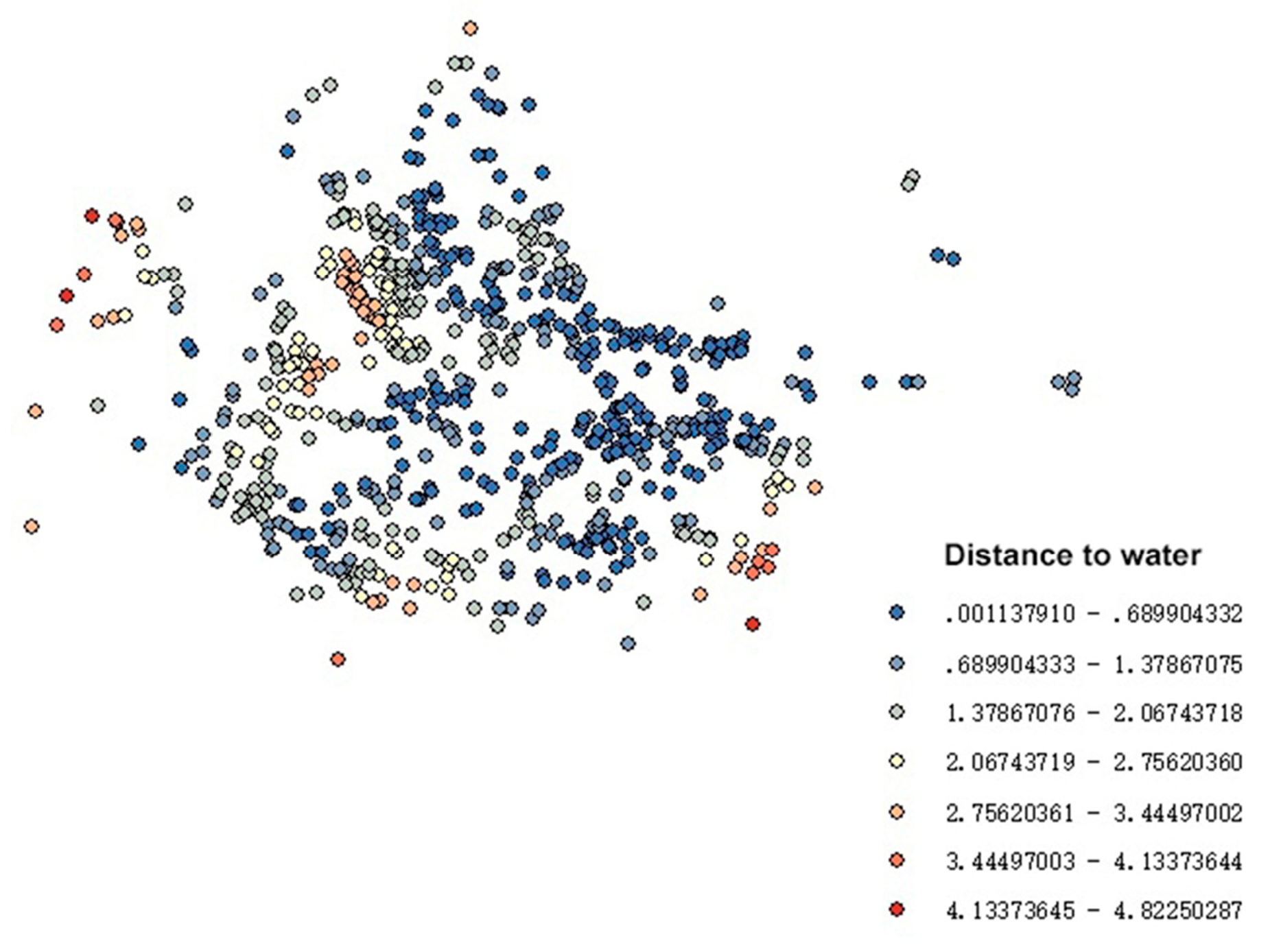
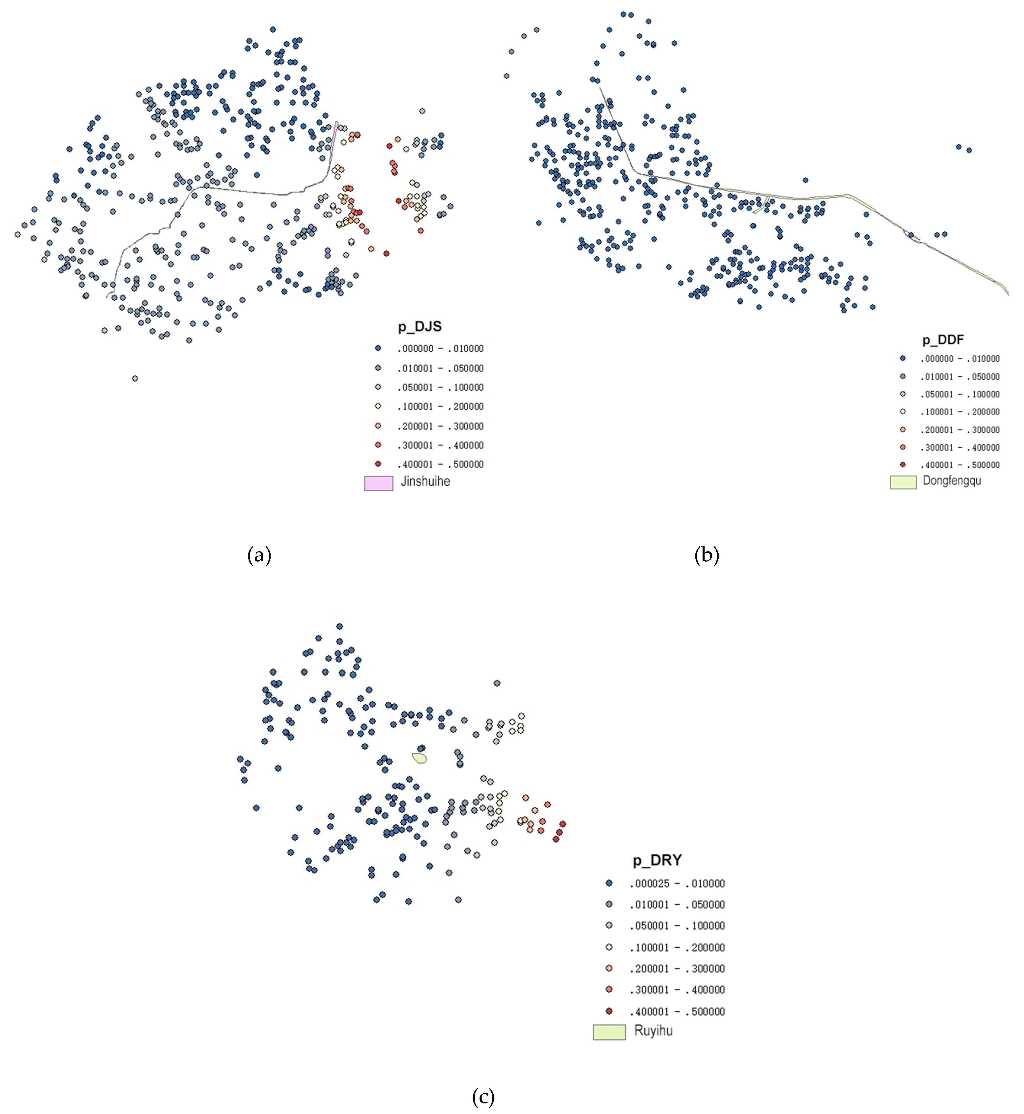
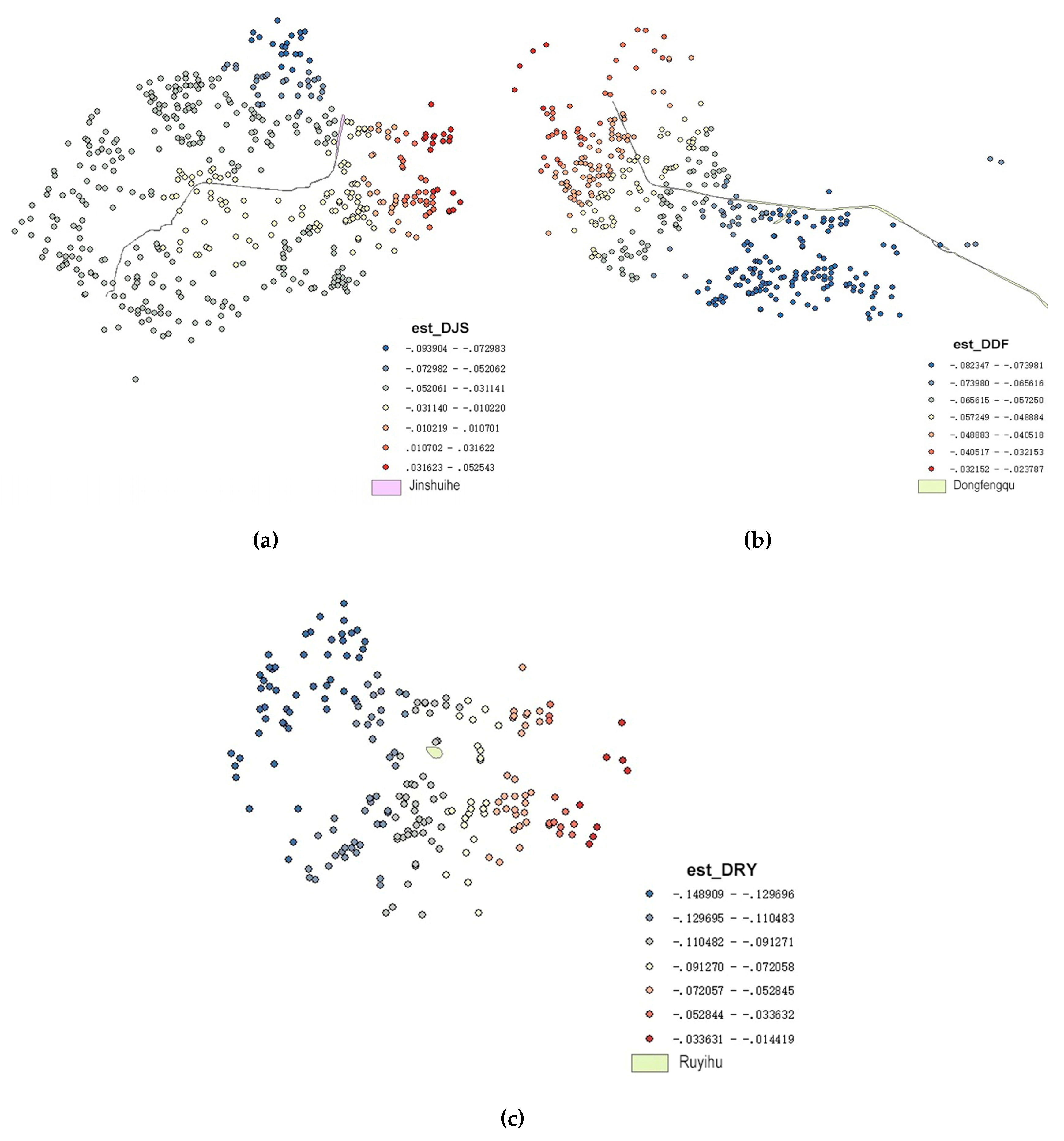
4.4. Results Analysis of Exploratory Research
5. Discussions and Conclusions
Author Contributions
Funding
Conflicts of Interest
References
- Goffette-Nagot, F.; Reginster, I.; Thomas, I. Spatial Analysis of Residential Land Prices in Belgium: Accessibility, Linguistic Border, and Environmental Amenities. Reg. Stud. 2011, 45, 1253–1268. [Google Scholar] [CrossRef]
- Maleki, M.Z.; Zain, M.F.M. Factors That Influence Distance to Facilities in a Sustainable Efficient Residential Site Design. Sustain. Cities Soc. 2011, 1, 236–243. [Google Scholar] [CrossRef]
- Liu, Z.; Robinson, G.M. Residential Development in the Peri-Urban Fringe: The Example of Adelaide, South Australia. Land Use Policy 2016, 57, 179–192. [Google Scholar] [CrossRef]
- Bonetti, F.; Corsi, S.; Orsi, L.; De Noni, I. Canals vs. Streams: To What Extent Do Water Quality and Proximity Affect Real Estate Values? A Hedonic Approach Analysis. Water 2016, 8, 577. [Google Scholar] [CrossRef]
- Loomis, J.; Feldman, M. Estimating the Benefits of Maintaining Adequate Lake Levels to Homeowners Using the Hedonic Property Method: Economic benefits of lake levels. Water Resour. Res. 2003, 39, 1–2. [Google Scholar] [CrossRef]
- Wen, H.; Bu, X.; Qin, Z. Spatial Effect of Lake Landscape on Housing Price: A Case Study of the West Lake in Hangzhou, China. Habitat Int. 2014, 44, 31–40. [Google Scholar] [CrossRef]
- Sander, H.A.; Polasky, S. The Value of Views and Open Space: Estimates from a Hedonic Pricing Model for Ramsey County, Minnesota, USA. Land Use Policy 2009, 26, 837–845. [Google Scholar] [CrossRef]
- Jiao, L.; Liu, Y. Geographic Field Model Based Hedonic Valuation of Urban Open Spaces in Wuhan, China. Landsc. Urban Plan. 2010, 98, 47–55. [Google Scholar] [CrossRef]
- Jim, C.Y.; Chen, W.Y. Impacts of Urban Environmental Elements on Residential Housing Prices in Guangzhou (China). Landsc. Urban Plan. 2006, 78, 422–434. [Google Scholar] [CrossRef]
- Tapsuwan, S.; Ingram, G.; Burton, M.; Brennan, D. Capitalized Amenity Value of Urban Wetlands: A Hedonic Property Price Approach to Urban Wetlands in Perth, Western Australia. Aust. J. Agric. Resour. Econ. 2009, 53, 527–545. [Google Scholar] [CrossRef]
- Hamilton, S.E.; Morgan, A. Integrating Lidar, GIS and Hedonic Price Modeling to Measure Amenity Values in Urban Beach Residential Property Markets. Comput. Environ. Urban Syst. 2010, 34, 133–141. [Google Scholar] [CrossRef]
- Jim, C.Y.; Chen, W.Y. External Effects of Neighbourhood Parks and Landscape Elements on High-Rise Residential Value. Land Use Policy 2010, 27, 662–670. [Google Scholar] [CrossRef]
- Luttik, J. The Value of Trees, Water and Open Space as Reflected by House Prices in the Netherlands. Landsc. Urban Plan. 2000, 7, 161–167. [Google Scholar] [CrossRef]
- Kashian, R.; Eiswerth, M.E.; Skidmore, M. Lake Rehabilitation and the Value of Shoreline Real Estate: Evidence from Delavan, Wisconsin. Rev. Reg. Stud. 2006, 36, 221–238. [Google Scholar]
- Ara, S.; Irwin, E.; Haab, T. Measuring the Effects of Lake Erie Water Quality in Spatial Hedonic Price Models. In Proceedings of the 3rd World Congress on Environmental and Resource Economics, Kyoto, Japan, 3–7 July 2006. [Google Scholar]
- Liao, F.; Wilhelm, F.; Solomon, M. The Effects of Ambient Water Quality and Eurasian Watermilfoil on Lakefront Property Values in the Coeur d’Alene Area of Northern Idaho, USA. Sustainability 2016, 8, 44. [Google Scholar] [CrossRef]
- Wen, H.; Xiao, Y.; Zhang, L. Spatial Effect of River Landscape on Housing Price: An Empirical Study on the Grand Canal in Hangzhou, China. Habitat Int. 2017, 63, 34–44. [Google Scholar] [CrossRef]
- Belanger, P.; Bourdeau-Brien, M. The Impact of Flood Risk on the Price of Residential Properties: The Case of England. Hous. Stud. 2018, 33, 876–901. [Google Scholar] [CrossRef]
- Daniel, V.E.; Florax, R.J.G.M.; Rietveld, P. Floods and Residential Property Values: A Hedonic Price Analysis for the Netherlands. Built Environ. 2009, 35, 563–576. [Google Scholar] [CrossRef]
- Hirsch, J.; Hahn, J. How Flood Risk Impacts Residential Rents and Property Prices: Empirical Analysis of a German Property Market. J. Prop. Investig. Financ. 2018, 36, 50–67. [Google Scholar] [CrossRef]
- Jung, E.; Yoon, H. Is Flood Risk Capitalized into Real Estate Market Value? A Mahalanobis-Metric Matching Approach to the Housing Market in Gyeonggi, South Korea. Sustainability 2018, 10, 4008. [Google Scholar] [CrossRef]
- Atreya, A.; Czajkowski, J. Graduated Flood Risks and Property Prices in Galveston County. Real Estate Econ. 2019, 47, 807–844. [Google Scholar] [CrossRef]
- Wen, H.; Jin, Y.; Zhang, L. Spatial Heterogeneity in Implicit Housing Prices: Evidence from Hangzhou, China. Int. J. Strateg. Prop. Manag. 2017, 21, 15–28. [Google Scholar] [CrossRef]
- Yu, H.; Huang, Y. Regional Heterogeneity and the Trans-Regional Interaction of Housing Prices and Inflation: Evidence from China’s 35 Major Cities. Urban Stud. 2016, 53, 3472–3492. [Google Scholar] [CrossRef]
- Nilsson, P. Natural Amenities in Urban Space—A Geographically Weighted Regression Approach. Landsc. Urban Plan. 2014, 121, 45–54. [Google Scholar] [CrossRef]
- Cohen, J.P.; Danko, J.J.; Yang, K. Proximity to a Water Supply Reservoir and Dams: Is There Spatial Heterogeneity in the Effects on Housing Prices? J. Hous. Econ. 2019, 43, 14–22. [Google Scholar] [CrossRef]
- Wen, H.; Xiao, Y.; Hui, E.C.M.; Zhang, L. Education Quality, Accessibility, and Housing Price: Does Spatial Heterogeneity Exist in Education Capitalization? Habitat Int. 2018, 78, 68–82. [Google Scholar] [CrossRef]
- R-Project.org. Documentation for Package ‘Stats’ Version 3.6.0. 2019. Available online: https://mirrors.tuna.tsinghua.edu.cn/CRAN/ (accessed on 16 May 2019).
- GeoDa 1.14. Documentation for Installation Package Version 1.14. 2019. Available online: http://geodacenter.github.io/download_windows.html (accessed on 21 July 2019).
- ArcGIS Online. Documentation for Installation Package Version Online. 2019. Available online: https://www.esri.com/en-us/arcgis/products/mapping (accessed on 23 July 2019).
- McMillen, D.P.; Redfearn, C.L. Estimation and hypothesis testing for nonparametric hedonic house price functions. J. Reg. Sci. 2010, 50, 712–733. [Google Scholar] [CrossRef]
- Brunsdon, C.; Fotheringham, A.S.; Charlton, M. Geographically Weighted Summary Statistics—a Framework for Localised Exploratory Data Analysis. Comput. Environ. Urban Syst. 2002, 26, 501–524. [Google Scholar] [CrossRef]
- Zhu, J.; Chen, B.; Lu, P.; Liu, J.; Tang, G. Impact of Urban Water System Treatment on the Surrounding Residential Land Price. Arab. J. Geosci. 2018, 11, 1–11. [Google Scholar] [CrossRef]
- Anderson, S.T.; West, S.E. Open Space, Residential Property Values, and Spatial Context. Reg. Sci. Urban Econ. 2006, 36, 773–789. [Google Scholar] [CrossRef]
- Harrison, C.; Eckman, B.; Hamilton, R.; Hartswick, P.; Kalagnanam, J.; Paraszczak, J.; Williams, P. Foundations for Smarter Cities. IBM J. Res. Dev. 2010, 54, 1–16. [Google Scholar] [CrossRef]
- Muvuna, J.; Boutaleb, T.; Baker, K.J.; Mickovski, S.B. A Methodology to Model Integrated Smart City System from the Information Perspective. Smart Cities 2019, 2, 496–511. [Google Scholar] [CrossRef]
- Malandrino, O.; Sica, D.; Supino, S. The Role of Public Administration in Sustainable Urban Development: Evidence from Italy. Smart Cities 2019, 2, 82–95. [Google Scholar] [CrossRef]


| Classification | Variable Name | Variable Type | Expected Sign |
|---|---|---|---|
| Structural factors | Building age | Continuous | Negative |
| Property category | Discrete | Negative | |
| Plot ratio | Continuous | Negative | |
| Property fee | Continuous | Positive | |
| Total number of houses | Discrete | Negative | |
| Greening rate | Continuous | Positive | |
| Total number of buildings | Discrete | Positive | |
| Location factors | Distance to CBD | Continuous | Negative |
| Distance to nearest top 3 Hospital | Continuous | Negative | |
| Distance to nearest business circle | Continuous | Negative | |
| Neighborhood factors | Number of bus stops within 500 m | Discrete | Positive |
| Number of supermarket within 500 m | Discrete | Positive | |
| Whether there is a metro station within 1 km | Discrete | Positive | |
| Whether there is a park within 1 km | Discrete | Positive | |
| Number of elementary school within 1 km | Discrete | Positive | |
| Number of junior high school within 1 km | Discrete | Positive | |
| Whether there is key school within 1 km | Discrete | Positive | |
| Water factors | Distance to water system | Continuous | Negative |
| Distance to river | Continuous | Negative | |
| Distance to lake | Continuous | Negative | |
| River surface width | Continuous | Positive | |
| Lake surface area | Continuous | Positive | |
| River water quality | Discrete | Negative |
| Classification | Variable Name | Unit | Average | Standard Deviation |
|---|---|---|---|---|
| Structural factors | Average price in the community | Yuan/m2 | 15,911 | 3568.4569 |
| Building age | Years | 12 | 4.2631 | |
| Property category | 0/1 | 0.99 | 0.0146 | |
| Plot ratio | —— | 3.93 | 0.0750 | |
| Property fee | Yuan/m2 | 1.22 | 0.6071 | |
| Total number of houses | Unit | 1315 | 848.1046 | |
| Greening rate | —— | 0.33 | 0.0576 | |
| Total number of buildings | Unit | 14 | 9.5716 | |
| Location factors | Distance to CBD | km | 10.97 | 3.9394 |
| Distance to nearest top 3 hospital | km | 1.72 | 0.7986 | |
| Distance to nearest business circle | km | 2.57 | 1.1837 | |
| Neighborhood factors | Number of bus stops within 500 m | Unit | 8 | 2.9497 |
| Number of supermarket within 500 m | Unit | 25 | 10.2882 | |
| Whether there is a metro station within 1 km | 0/1 | 0.27 | 0.3928 | |
| Whether there is a park within 1 km | 0/1 | 0.86 | 0.2452 | |
| Number of elementary school within 1 km | Unit | 2.71 | 1.3817 | |
| Number of junior high school within 1 km | Unit | 2.00 | 1.4357 | |
| Whether there is key school within 1 km | 0/1 | 0.25 | 0.3728 | |
| Water factors | Distance to water system | km | 1.21 | 0.7646 |
| Distance to river | km | 1.21 | 0.7687 | |
| Distance to lake | km | 4.41 | 1.7499 | |
| River surface width | m | 28.79 | 8.7005 | |
| Lake surface area | 10,000 m2 | 76.14 | 85.4995 | |
| River water quality | Level | 3.78 | 0.6042 |
| Name of Model | Setting of Model |
|---|---|
| Model 1 | |
| Model 2 | |
| Model 3 | |
| Model 4 | |
| Model 5 | |
| Model 6 | |
| Model 7 |
| Model 1 | Model 2 | Model 3 | Model 4 | Model 5 | Model 6 | |
|---|---|---|---|---|---|---|
| R-square | 0.6414 | 0.6872 | 0.6528 | 0.6906 | 0.6393 | 0.6887 |
| Adjusted R-square | 0.6316 | —— | 0.6428 | —— | 0.6284 | —— |
| Prob(F-statistic) | 0.0000 | —— | 0.0000 | —— | 0.0000 | —— |
| Log likelihood | 284.0520 | 324.0610 | 294.9640 | 328.5710 | 282.0740 | 324.8570 |
| Akaike info criterion | −530.1000 | −608.1230 | −549.9270 | −615.1430 | −522.1480 | −605.7150 |
| Schwarz criterion | −444.2400 | −517.7400 | −459.5440 | −520.2400 | −427.2460 | −506.2940 |
| Model 1 | Model 2 | ||||
|---|---|---|---|---|---|
| Variable Name | Standard Coefficient | p-Value | VIF [c] | Standard Coefficient | p-Value |
| Constant | 11.1037 | 0.0000 | —— | 6.2393 | 0.0000 |
| Building age | −0.0164 | 0.0000 | 2.8060 | −0.0160 | 0.0000 |
| Property category | −0.2431 | 0.0032 | 1.2820 | −0.3217 | 0.0000 |
| Plot ratio | −0.0622 | 0.0018 | 2.2902 | −0.0495 | 0.0069 |
| Property fee | 0.1003 | 0.0000 | 2.5632 | 0.0843 | 0.0000 |
| Total number of houses | −0.0727 | 0.0000 | 2.8700 | −0.0607 | 0.0000 |
| Greening rate | 0.0493 | 0.0302 | 1.1425 | 0.0576 | 0.0058 |
| Total number of buildings | 0.1068 | 0.0000 | 3.0829 | 0.0913 | 0.0000 |
| Distance to CBD | −0.2714 | 0.0000 | 1.5551 | −0.1575 | 0.0000 |
| Distance to nearest top 3 Hospital | −0.0431 | 0.0001 | 1.4016 | −0.0377 | 0.0001 |
| Distance to nearest business circle | −0.0814 | 0.0000 | 1.4719 | −0.0637 | 0.0000 |
| Number of bus stops within 500 m | 0.0012 | 0.5534 | 1.3822 | −0.0017 | 0.3688 |
| Number of supermarkets within 500 m | −0.0026 | 0.0000 | 1.6703 | −0.0010 | 0.0789 |
| Whether there is a metro station within 1 km | −0.0214 | 0.1603 | 1.1840 | −0.0122 | 0.3836 |
| Whether there is a park within 1 km | 0.0334 | 0.0758 | 1.1222 | 0.0393 | 0.0229 |
| Number of elementary schools within 1 km | −0.0020 | 0.6461 | 1.4811 | 0.0026 | 0.5197 |
| Number of junior high school within 1 km | 0.0264 | 0.0000 | 1.4111 | 0.0216 | 0.0000 |
| Whether there is key school within 1 km | 0.0522 | 0.0004 | 1.0552 | 0.0422 | 0.0019 |
| Distance to water system | −0.0278 | 0.0000 | 1.1721 | −0.0214 | 0.0002 |
| W*lnP | —— | —— | —— | 0.4761 | 0.0000 |
| Model 3 | Model 4 | ||||
|---|---|---|---|---|---|
| Variable Name | Standard Coefficient | p-Value | VIF[c] | Standard Coefficient | p-Value |
| Constant | 11.1488 | 0.0000 | —— | 6.5951 | 0.0000 |
| Building age | −0.0166 | 0.0000 | 2.8070 | −0.0161 | 0.0000 |
| Property category | −0.2735 | 0.0008 | 1.2910 | −0.3347 | 0.0000 |
| Plot ratio | −0.0591 | 0.0027 | 2.0990 | −0.0488 | 0.0075 |
| Property fee | 0.0978 | 0.0000 | 2.5676 | 0.0839 | 0.0000 |
| Total number of houses | −0.0705 | 0.0000 | 2.8735 | −0.0601 | 0.0000 |
| Greening rate | 0.0572 | 0.0111 | 1.1514 | 0.0616 | 0.0031 |
| Total number of buildings | 0.1036 | 0.0000 | 3.0925 | 0.0904 | 0.0000 |
| Distance to CBD | −0.2630 | 0.0000 | 1.5786 | −0.1600 | 0.0000 |
| Distance to nearest top 3 hospital | −0.0353 | 0.0011 | 1.4422 | −0.0334 | 0.0008 |
| Distance to nearest business circle | −0.0628 | 0.0000 | 1.6936 | −0.0537 | 0.0000 |
| Number of bus stops within 500 m | 0.0005 | 0.7872 | 1.3904 | −0.0019 | 0.3144 |
| Number of supermarkets within 500 m | −0.0020 | 0.0013 | 1.7589 | −0.0008 | 0.1889 |
| Whether there is a metro station within 1 km | −0.0292 | 0.0537 | 1.1985 | −0.0176 | 0.2097 |
| Whether there is a park within 1 km | 0.0346 | 0.0617 | 1.1225 | 0.0397 | 0.0210 |
| Number of elementary schools within 1 km | 0.0026 | 0.5666 | 1.5616 | 0.0051 | 0.2230 |
| Number of junior high schools within 1 km | 0.0294 | 0.0000 | 1.4565 | 0.0238 | 0.0000 |
| Whether there is key school within 1 km | 0.0502 | 0.0006 | 1.0561 | 0.0417 | 0.0021 |
| Distance to river | −0.0231 | 0.0002 | 1.2160 | −0.0192 | 0.0010 |
| Distance to lake | −0.0568 | 0.0000 | 1.5949 | −0.0342 | 0.0039 |
| W*lnP | —— | —— | —— | 0.4439 | 0.0000 |
| Model 5 | Model 6 | ||||
|---|---|---|---|---|---|
| Variable Name | Standard Coefficient | p-Value | VIF[c] | Standard Coefficient | p-Value |
| Constant | 11.1992 | 0.0000 | —— | 6.1310 | 0.0000 |
| Building age | −0.0171 | 0.0000 | 2.8840 | −0.0169 | 0.0000 |
| Property category | −0.2646 | 0.0016 | 1.3079 | −0.3559 | 0.0000 |
| Plot ratio | −0.0563 | 0.0050 | 2.1059 | −0.0474 | 0.0097 |
| Property fee | 0.0983 | 0.0000 | 2.5671 | 0.0824 | 0.0000 |
| Total number of houses | −0.0735 | 0.0000 | 2.8832 | −0.0593 | 0.0000 |
| Greening rate | 0.0443 | 0.0535 | 1.1510 | 0.0541 | 0.0098 |
| Total number of buildings | 0.1082 | 0.0000 | 3.0879 | 0.0922 | 0.0000 |
| Distance to CBD | −0.2869 | 0.0000 | 1.9000 | −0.1503 | 0.0000 |
| Distance to nearest top 3 hospital | −0.0342 | 0.0020 | 1.4594 | −0.0327 | 0.0012 |
| Distance to nearest business circle | −0.0804 | 0.0000 | 1.5764 | −0.0575 | 0.0000 |
| Number of bus stops within 500 m | 0.0016 | 0.4211 | 1.3906 | −0.0017 | 0.3613 |
| Number of supermarkets within 500 m | −0.0023 | 0.0003 | 1.7546 | −0.0010 | 0.0924 |
| Whether there is a metro station within 1 km | −0.0156 | 0.3117 | 1.1954 | −0.0045 | 0.7465 |
| Whether there is a park within 1 km | 0.0336 | 0.0763 | 1.1350 | 0.0366 | 0.0350 |
| Number of elementary schools within 1 km | −0.0052 | 0.2507 | 1.5644 | −0.0013 | 0.7622 |
| Number of junior high schools within 1 km | 0.0242 | 0.0000 | 1.4238 | 0.0203 | 0.0000 |
| Whether there is key school within 1 km | 0.0432 | 0.0045 | 1.1037 | 0.0347 | 0.0123 |
| River surface width | 0.0021 | 0.0062 | 1.5138 | 0.0013 | 0.0633 |
| Lake surface area | −0.0003 | 0.6919 | 1.6910 | −0.0001 | 0.1015 |
| River water quality | −0.0244 | 0.0384 | 1.7957 | −0.0357 | 0.0009 |
| W*lnP | —— | —— | —— | 0.5010 | 0.0000 |
| Water System Accessibility | River and Lake Accessibility | Nature of the Water System | |
|---|---|---|---|
| R-square | 0.6145 | 0.6174 | 0.5687 |
| Adjusted R-square | 0.6054 | 0.6089 | 0.5601 |
| Akaike info criterion | −486.3656 | −491.5502 | −415.6654 |
© 2020 by the authors. Licensee MDPI, Basel, Switzerland. This article is an open access article distributed under the terms and conditions of the Creative Commons Attribution (CC BY) license (http://creativecommons.org/licenses/by/4.0/).
Share and Cite
Li, J.; Hu, Y.; Liu, C. Exploring the Influence of an Urban Water System on Housing Prices: Case Study of Zhengzhou. Buildings 2020, 10, 44. https://doi.org/10.3390/buildings10030044
Li J, Hu Y, Liu C. Exploring the Influence of an Urban Water System on Housing Prices: Case Study of Zhengzhou. Buildings. 2020; 10(3):44. https://doi.org/10.3390/buildings10030044
Chicago/Turabian StyleLi, Junjie, Yaduo Hu, and Chunlu Liu. 2020. "Exploring the Influence of an Urban Water System on Housing Prices: Case Study of Zhengzhou" Buildings 10, no. 3: 44. https://doi.org/10.3390/buildings10030044
APA StyleLi, J., Hu, Y., & Liu, C. (2020). Exploring the Influence of an Urban Water System on Housing Prices: Case Study of Zhengzhou. Buildings, 10(3), 44. https://doi.org/10.3390/buildings10030044