Optimising Window Design on Residential Building Facades by Considering Heat Transfer and Natural Lighting in Nontropical Regions of Australia


Abstract

1. Introduction
2. Literature Review
2.1. Optimisation Technique
2.2. Window Lighting and Thermal Effects
3. Methodology
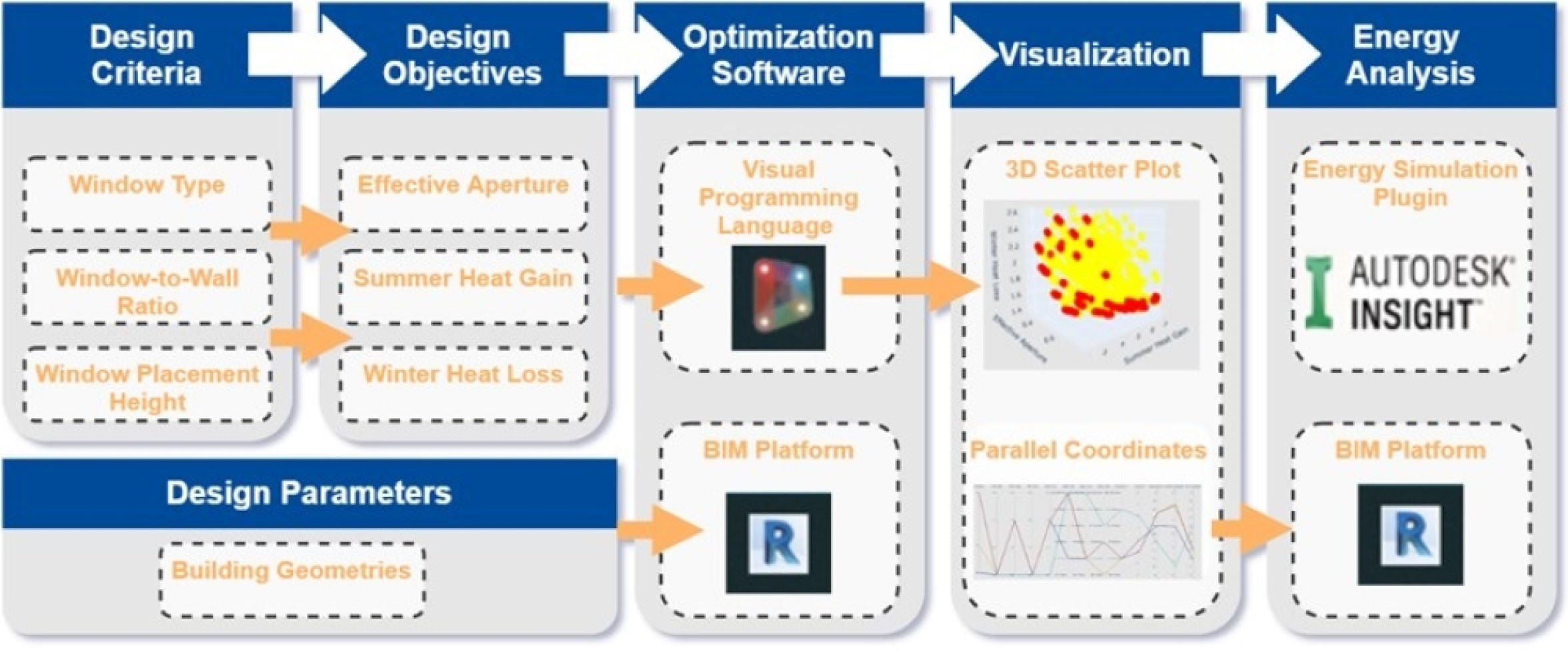
3.1. Optimisation Framework
- On each story level, windows facing the same direction should be placed at the same height.
- The overall window system is installed with the same type of window.
- Shading devices attached on the same wall face have the same width, measured as the perpendicular distance from the edge of the shading device to the wall [56].
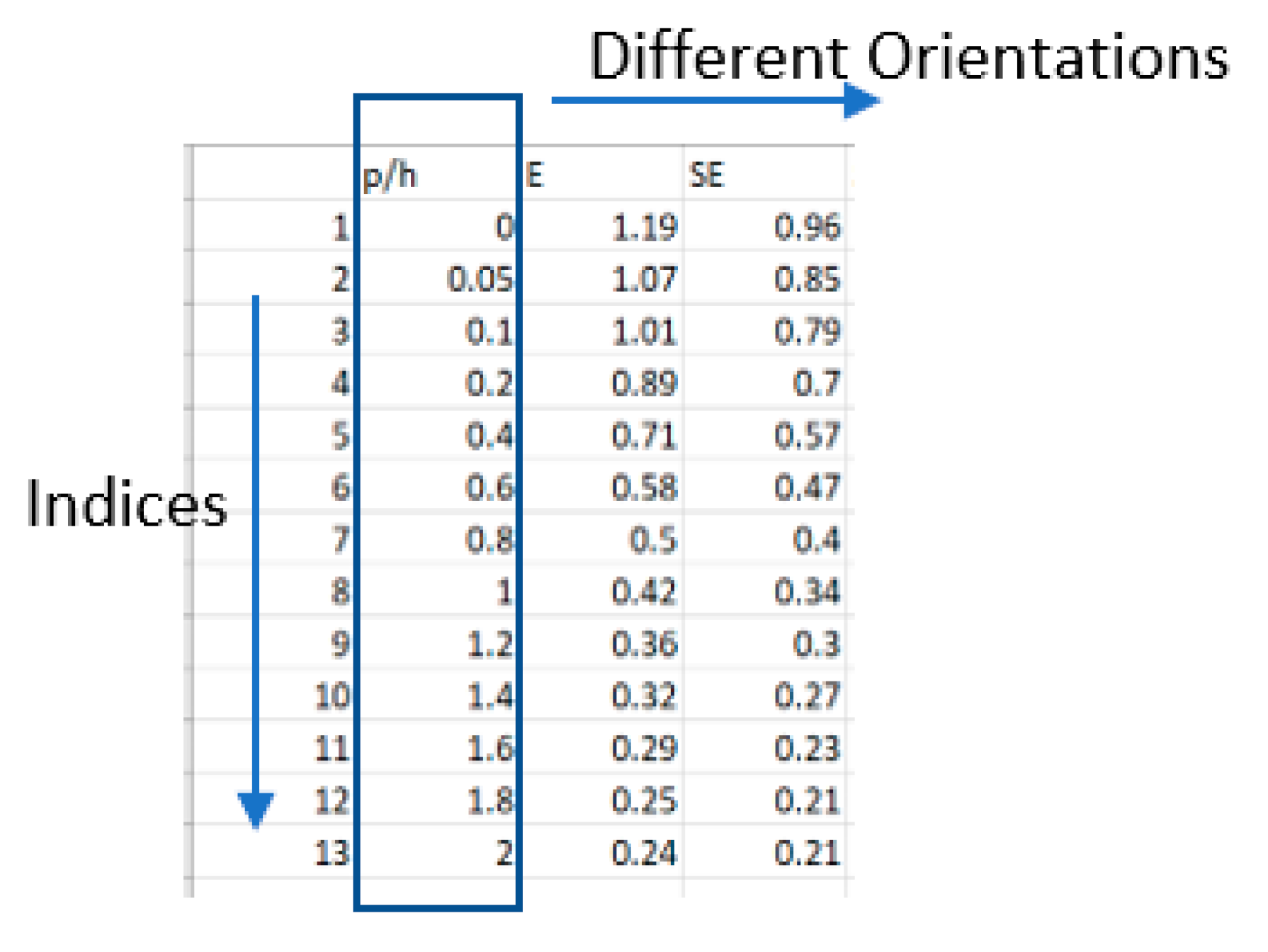
3.2. Computing Effective Aperture
3.3. Computing Summer Heat Gain and Winter Heat Loss
3.4. Model Constraints
3.4.1. Window Placement Constraint
3.4.2. Window-To-Floor Ratio (WFR) Constraint
3.4.3. Maximum Thermal Values Constraint
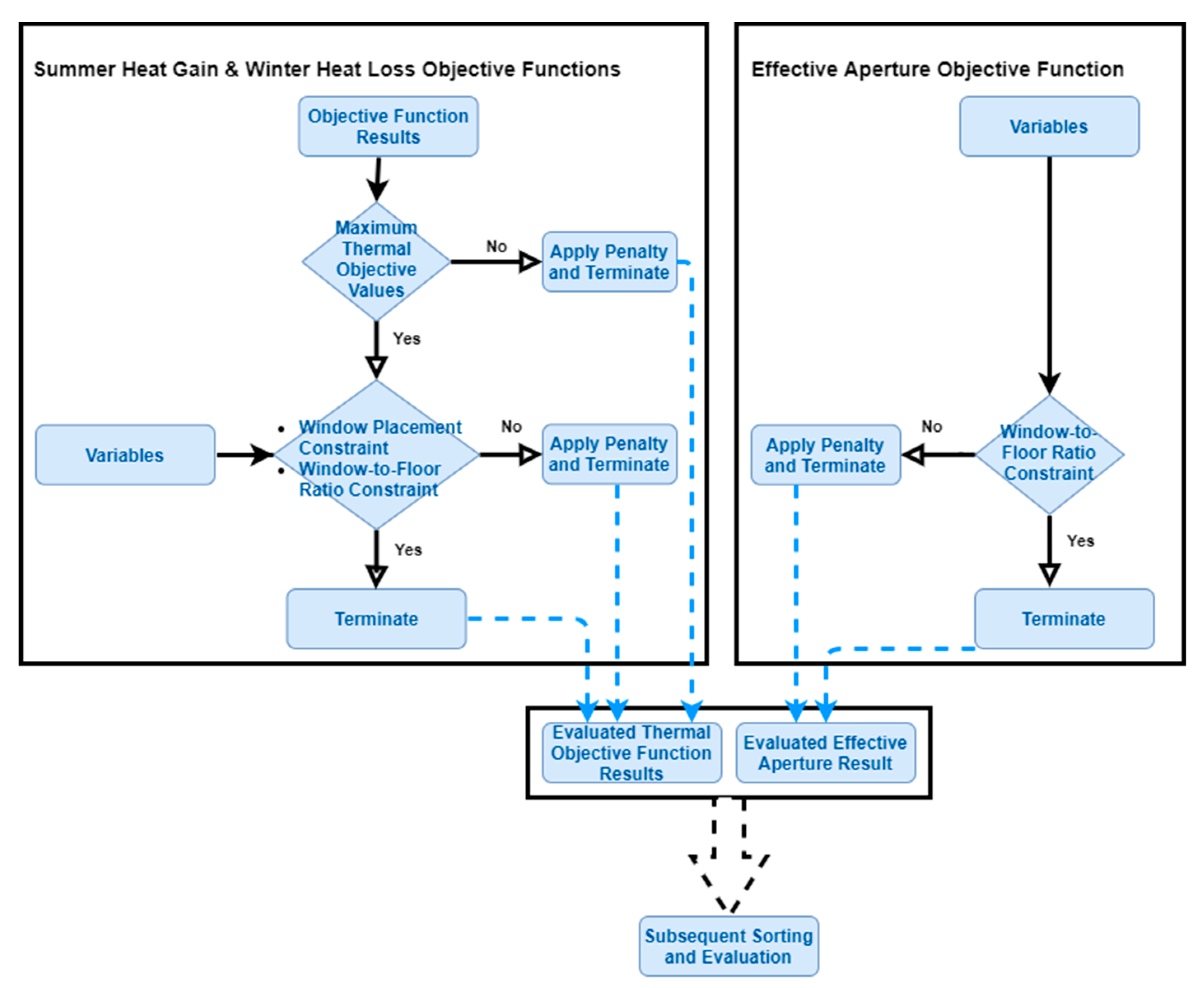
3.5. Penalty Function
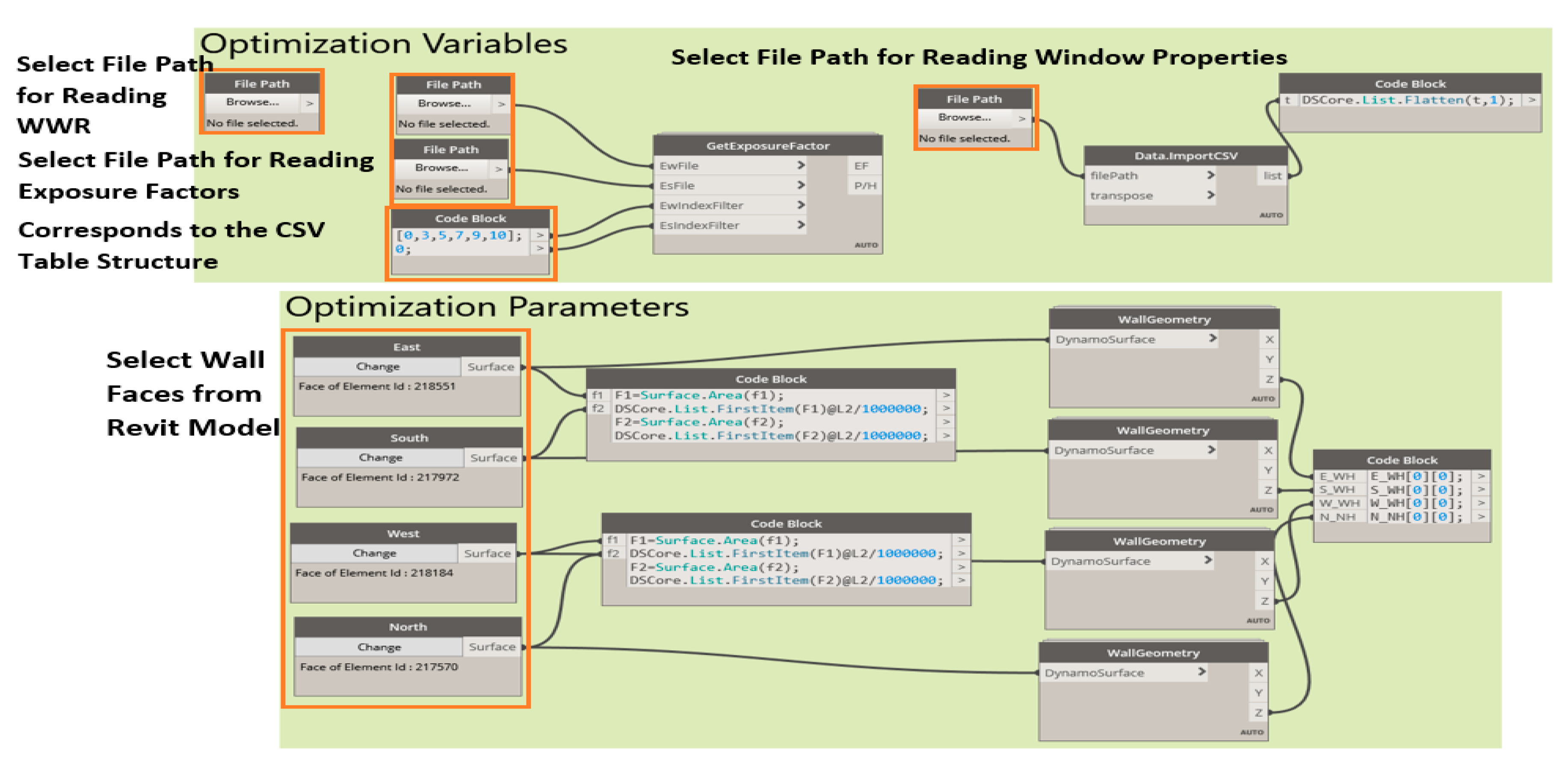
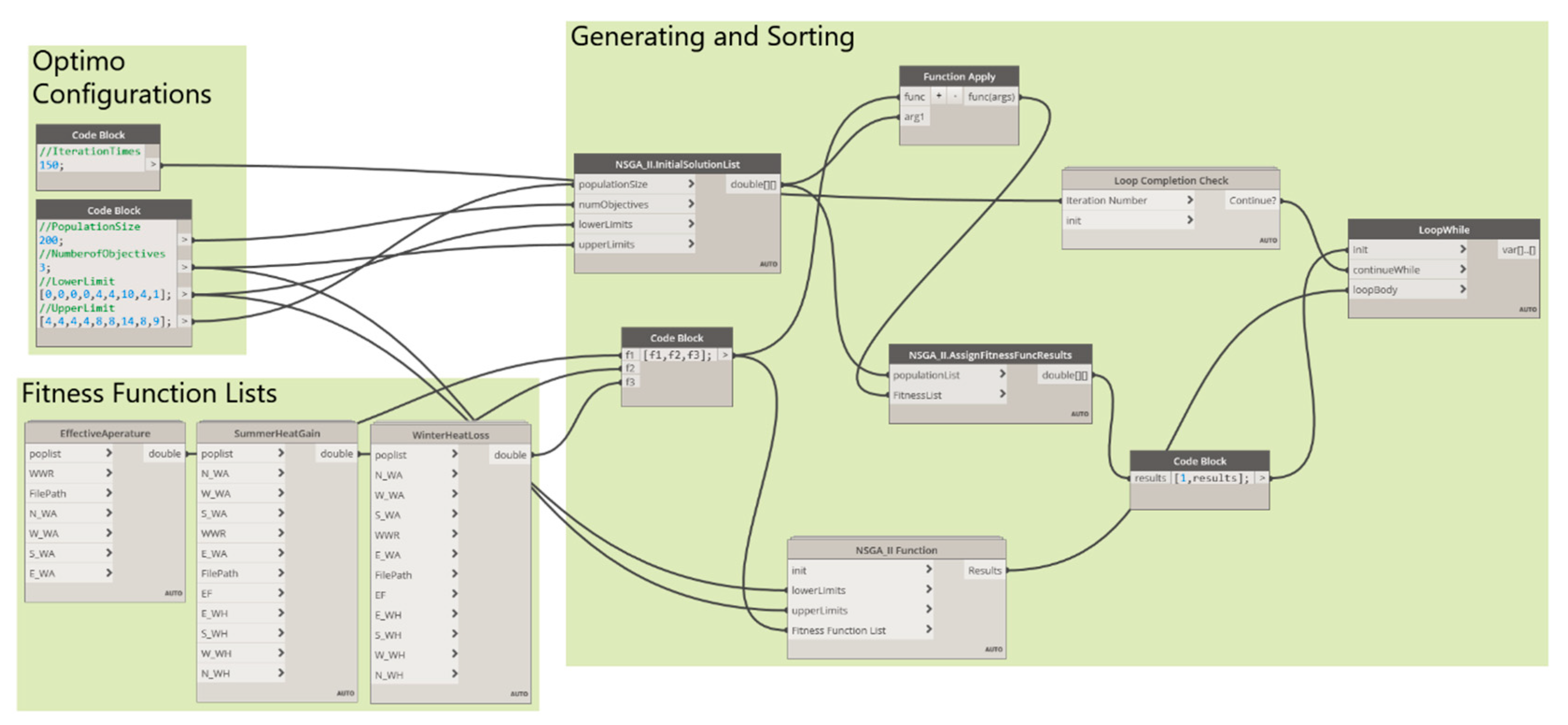
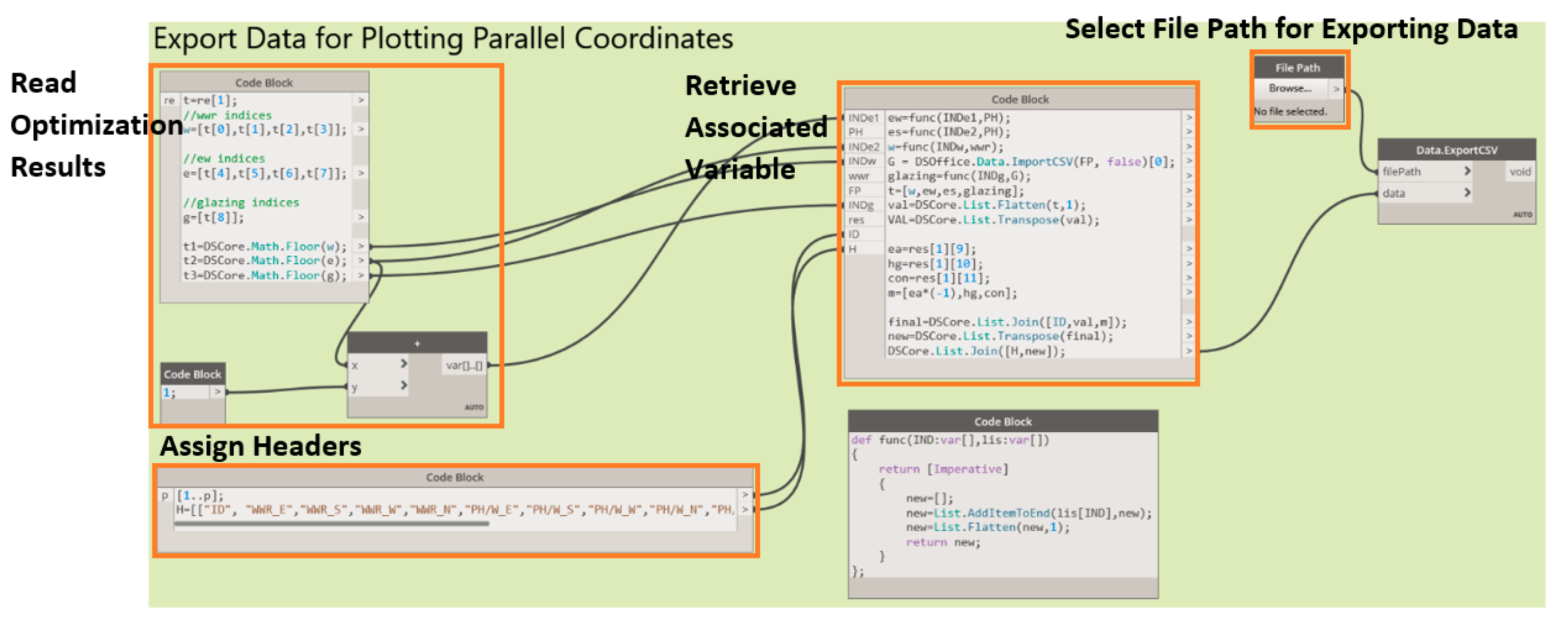
3.6. Dynamo Workflow
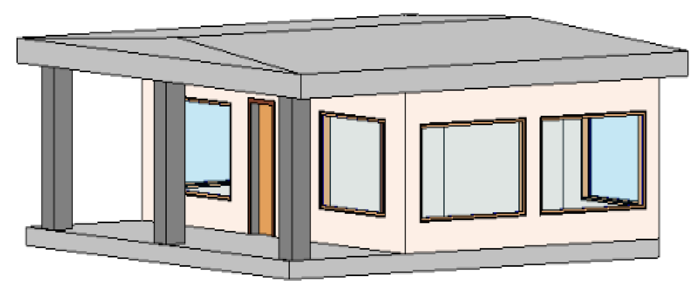
4. Case Study
4.1. Variable Selection
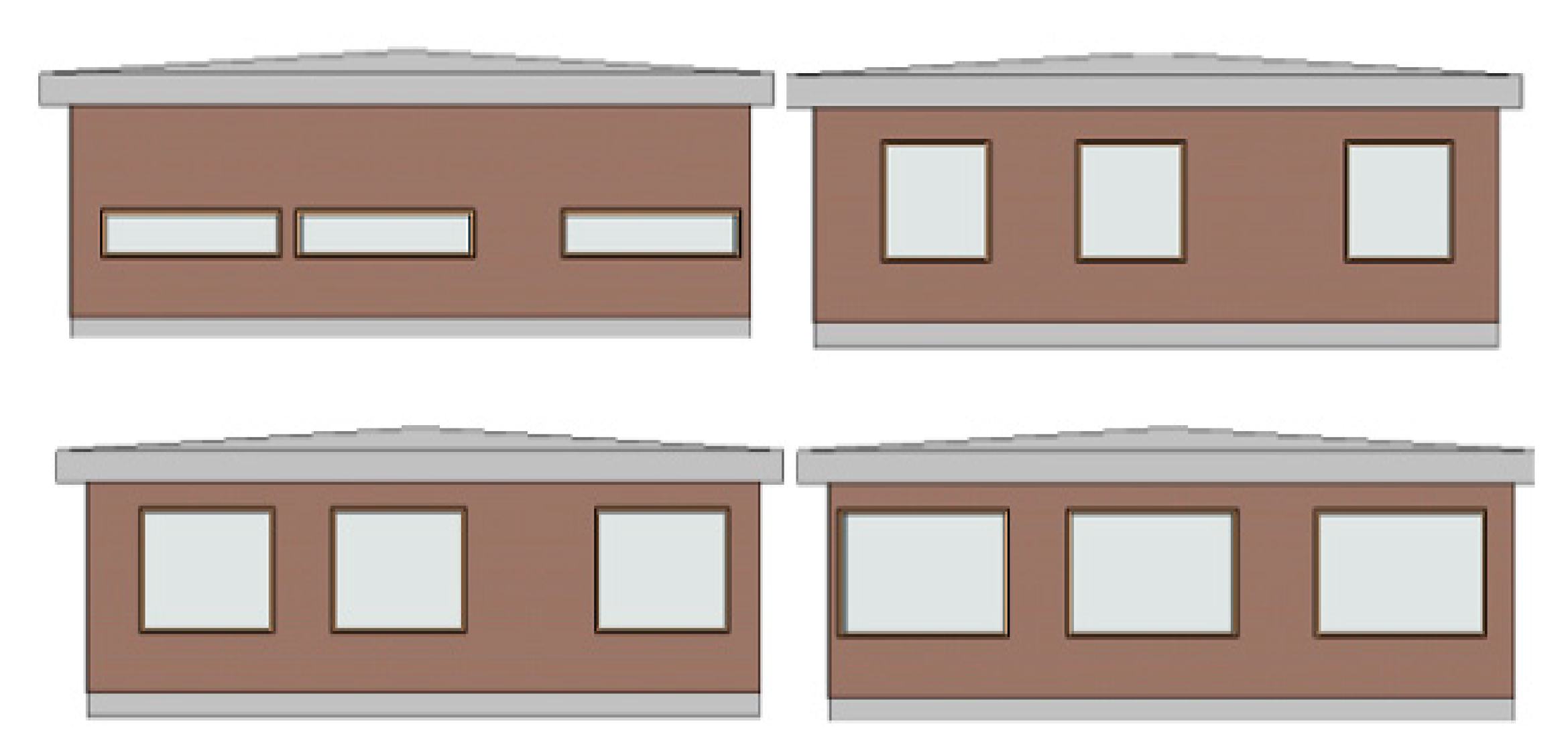
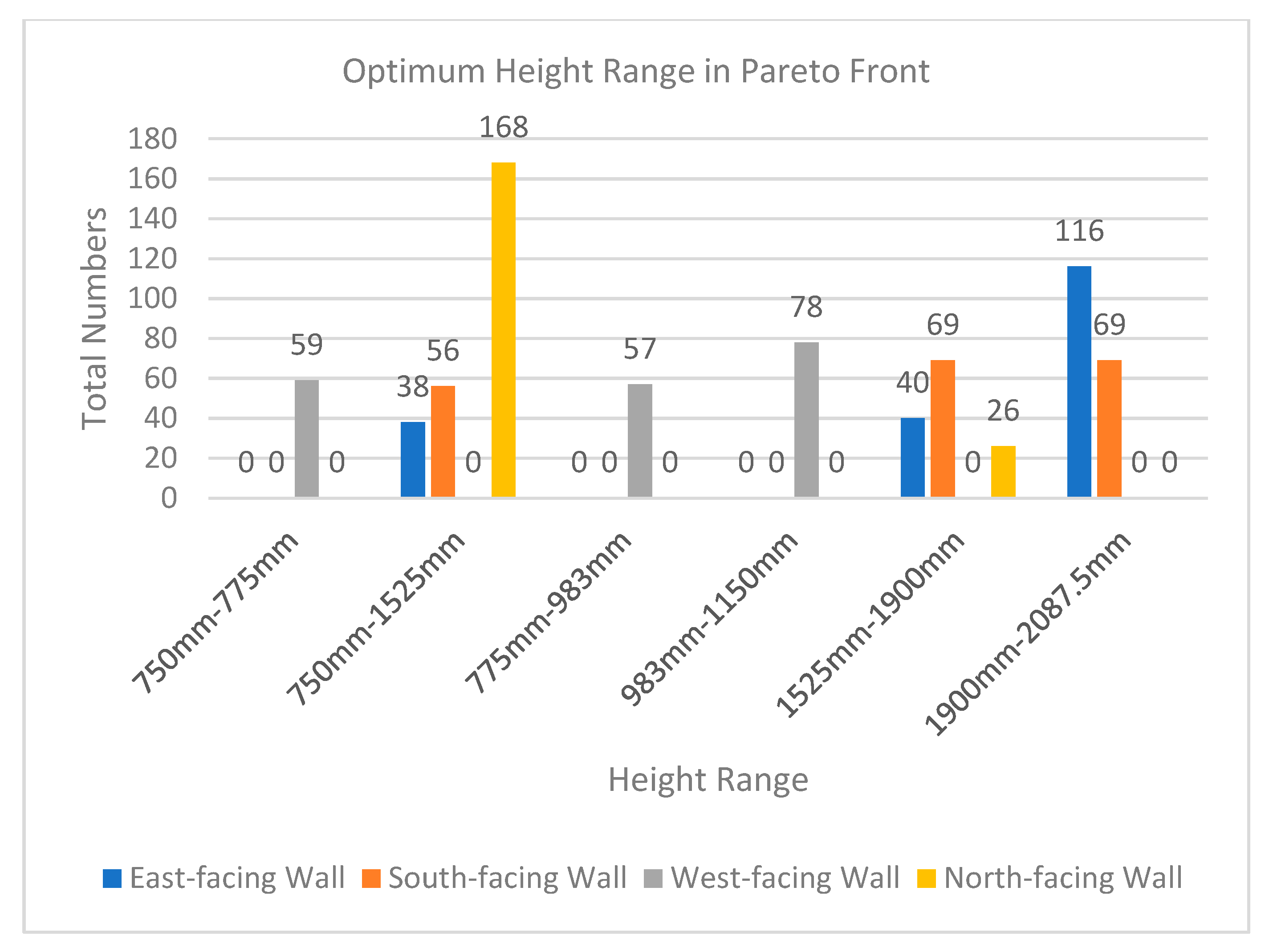
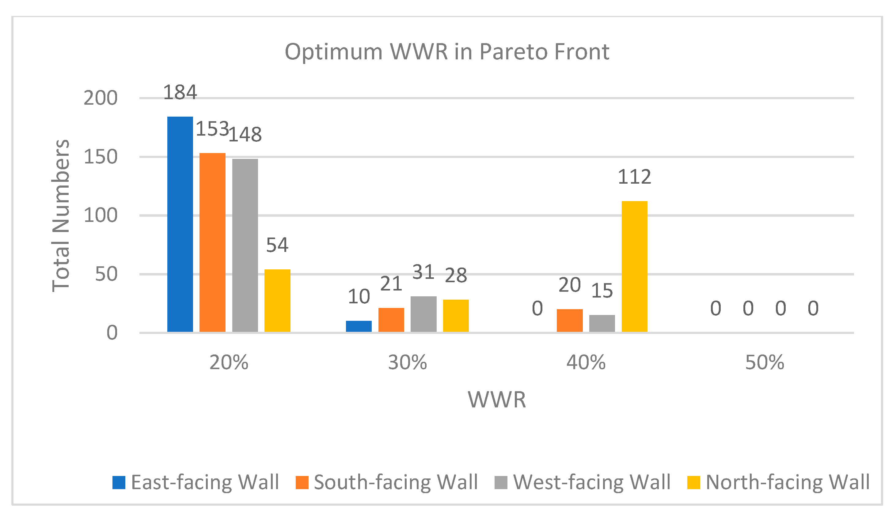
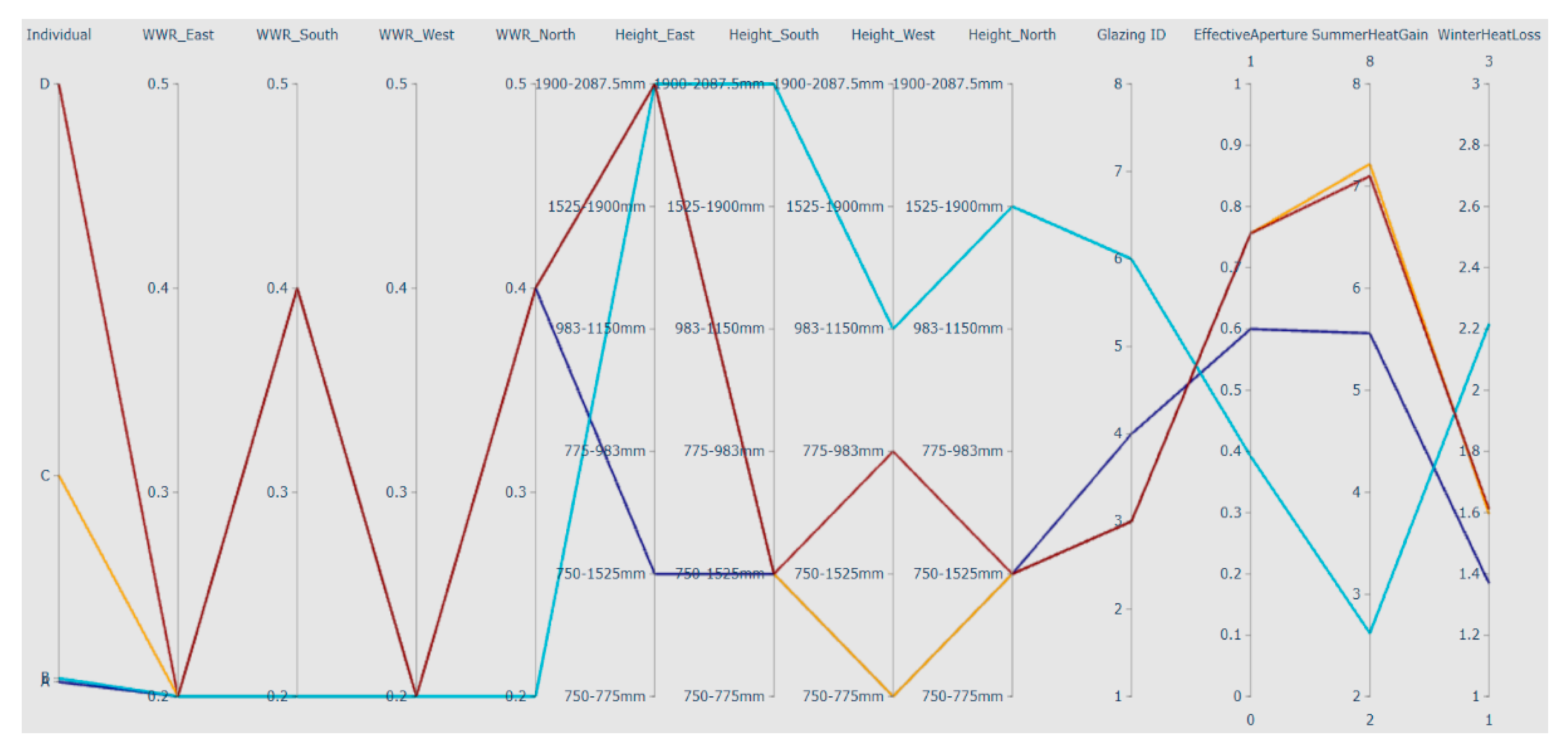
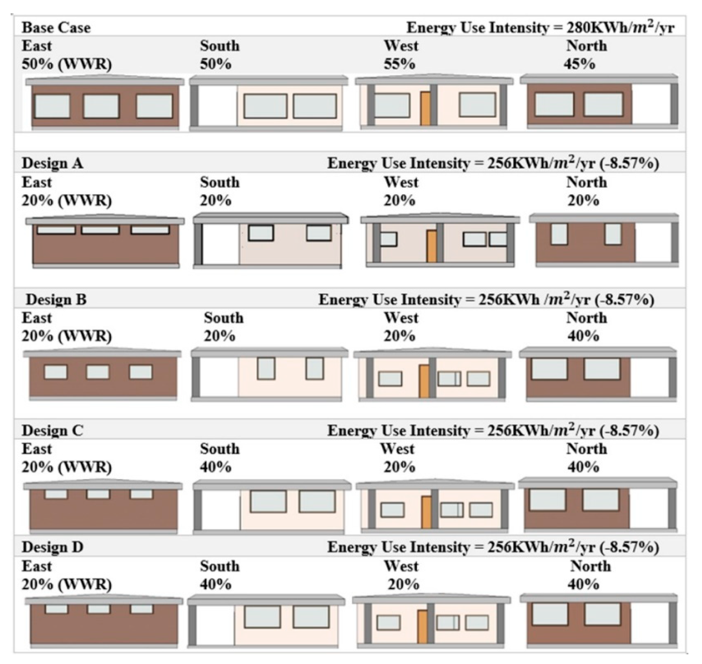
4.2. Results and Discussion
4.3. Sensitivity Analysis
5. Conclusions
Author Contributions
Funding
Conflicts of Interest
Nomenclature
| ABBREVIATIONS | |
| BIM | Building Information Modelling |
| CSV | Comma-separated Value file format |
| GBI | Green Building Initiative |
| HVAC | Heating, ventilation and air conditioning |
| IFC | Industry Foundation Classes |
| MOO | Multi-objective Optimisation |
| NCC | National Construction Code |
| NSGA-II | Non-Dominated Sorting Genetic Algorithm |
| SHGC | Solar Heat Gain Coefficient |
| SRC | Standardised Regression Coefficients |
| VLT | Visual Light Transmittance |
| VPL | Visual Programming Language |
| U | Overall Heat Transfer Coefficient |
| WFR | Window-to-Floor Ratio |
| WWR | Window-to-Wall Ratio |
| SET | |
| Set of walls with windows scheduled on each story | |
| OBJECTIVE FUNCTIONS | |
| Effective aperture calculated on each floor | |
| A general function for calculating overall heat gain in Watts | |
| A general function for calculating overall heat loss in Watts | |
| Winter heat loss calculated on each floor | |
| Summer heat gain calculated on each floor | |
| VARIABLES | |
| Visual light transmittance for the window system | |
| Solar heat gain coefficient for the window system | |
| Overall heat transfer coefficient for the window system ( | |
| WWR scheduled for the wall | |
| Summer exposure factor of the wall | |
| Winter exposure factor of the wall | |
| Binary variable which is equal to 1 when summer heat gain exceeds the maximum value allowed, and 0 otherwise | |
| Binary variable which is equal to 1 when winter heat loss exceeds the maximum value allowed, and 0 otherwise | |
| Binary variable which is equal to one when the window placement constraint is violated, and 0 otherwise | |
| Binary variable which is equal to one when the window-to-floor ratio constraint is violated, and 0 otherwise | |
| PARAMETERS | |
| Total window area on each story | |
| Solar irradiance | |
| The width of the shading device | |
| The distance between the base of the window to the bottom of the shading device | |
| Gross area of the hosting wall | |
| Height of the hosting wall | |
| A hypothetical working plane determined by the designer | |
| Lower bound for window placement on the wall | |
| Upper bound for window placement on the wall | |
| The minimum WFR specified by the designer | |
| The maximum WFR specified by the designer | |
| The fully enclosed covered area on each floor | |
| Maximum value allowed for summer heat gain | |
| Deemed-to-satisfy constant for calculating summer heat gain obtained from the National Construction Code (NCC) | |
| Maximum value allowed for winter heat loss | |
| Deemed-to-satisfy constant for calculating winter heat loss obtained from the National Construction Code (NCC) | |
| Constant penalty | |
| PENALTY FUNCTIONS | |
| Penalty function applied to the design objective summer heat gain | |
| Penalty function applied to the design objective winter heat loss | |
| Penalty function applied to the design objective effective aperture | |
References
- UNEP DTIE Sustainable Consumption & Production Branch. Buildings and Climate Change Summary for Decision-Makers (p. 5). United Nations Environment Programme. 2009. Available online: https://ledsgp.org/wp-content/uploads/2015/07/buildings-and-climate-change.pdf (accessed on 16 November 2020).
- US Energy Information Administration. International Energy Outlook 2016 (p. 101). US Enegry Information Administration. 2015. Available online: https://www.eia.gov/outlooks/ieo/pdf/buildings.pdf (accessed on 16 November 2020).
- Australian Building Codes Board. ABCB Building Classifications; Australian Building Codes Board: Canberra, Australian, 2020. [Google Scholar]
- Energy Account, Australia, 2017–2018 Financial Year|Australian Bureau of Statistics. Available online: https://www.abs.gov.au/statistics/industry/energy/energy-account-australia/latest-release (accessed on 12 November 2019).
- Tian, Z.; Zhang, X.; Jin, X.; Zhou, X.; Si, B.; Shi, X. Towards adoption of building energy simulation and optimization for passive building design: A survey and a review. Energy Build. 2018, 158, 1306–1316. [Google Scholar] [CrossRef]
- Gou, S.; Nik, V.M.; Scartezzini, J.-L.; Zhao, Q.; Li, Z. Passive design optimization of newly-built residential buildings in Shanghai for improving indoor thermal comfort while reducing building energy demand. Energy Build. 2018, 169, 484–506. [Google Scholar] [CrossRef]
- AlBayyaa, H.; Hagare, D.; Saha, S. Energy conservation in residential buildings by incorporating Passive Solar and Energy Efficiency Design Strategies and higher thermal mass. Energy Build. 2019, 182, 205–213. [Google Scholar] [CrossRef]
- Cuce, E. Role of airtightness in energy loss from windows: Experimental results from in-situ tests. Energy Build. 2017, 139, 449–455. [Google Scholar] [CrossRef]
- Arasteh, D.; Selkowitz, S.; Apte, J.; LaFrance, M. Zero Energy Windows; Ernest Orlando Lawrence Berkeley National Laboratory: Berkeley, CA, USA, 2006; Volume 14. [Google Scholar]
- Johnston, D.; Zhang, H.; Airah, M.; Wang, G.; Bannister, P.; Airah, F. Glazing Studies for The National Construction Code 2019. In Proceedings of the AIRAH and IBPSA’s Australasian Building Simulation 2017 Conference, Melbourne, Australia, 15–16 November 2017. [Google Scholar]
- Chen, X.; Yang, H.; Wang, T. Developing a robust assessment system for the passive design approach in the green building rating scheme of Hong Kong. J. Clean. Prod. 2017, 153, 176–194. [Google Scholar] [CrossRef]
- Kolarik, J.; Toftum, J.; Olesen, B.W.; Jensen, K.L. Simulation of energy use, human thermal comfort and office work performance in buildings with moderately drifting operative temperatures. Energy Build. 2011, 43, 2988–2997. [Google Scholar] [CrossRef]
- Kim, S.; Zadeh, P.A.; Staub-French, S.; Froese, T.M.; Cavka, B.T. Assessment of the Impact of Window Size, Position and Orientation on Building Energy Load Using BIM. Procedia Eng. 2016, 145, 1424–1431. [Google Scholar] [CrossRef]
- Ashrafian, T.; Moazzen, N. The impact of glazing ratio and window configuration on occupants’ comfort and energy demand: The case study of a school building in Eskisehir, Turkey. Sustain. Cities Soc. 2019, 47, 101483. [Google Scholar] [CrossRef]
- Mahar, W.A.; Verbeeck, G.; Reiter, S.; Attia, S. Sensitivity Analysis of Passive Design Strategies for Residential Buildings in Cold Semi-Arid Climates. Sustainability 2020, 12, 1091. [Google Scholar] [CrossRef]
- Reilly, M.; Winkelmann, F.; Arasteh, D.; Carroll, W. Modeling windows in DOE-2.1E. Energy Build. 1995, 22, 59–66. [Google Scholar] [CrossRef]
- Cheung, C.; Fuller, R.; Luther, M. Energy-efficient envelope design for high-rise apartments. Energy Build. 2005, 37, 37–48. [Google Scholar] [CrossRef]
- Dutta, A.; Samanta, A. Reducing cooling load of buildings in the tropical climate through window glazing: A model to model comparison. J. Build. Eng. 2018, 15, 318–327. [Google Scholar] [CrossRef]
- Bokel, R.M.J. The Effect of Window Position and Window Size on The Energy Demand for Heating, Cooling and Electric Lighting. Build. Simulat. 2007, 10, 117–121. [Google Scholar]
- Sun, Y.; Shanks, K.; Baig, H.; Zhang, W.; Hao, X.; Li, Y.; He, B.; Wilson, R.; Liu, H.; Sundaram, S.; et al. Integrated semi-transparent cadmium telluride photovoltaic glazing into windows: Energy and daylight performance for different architecture designs. Appl. Energy 2018, 231, 972–984. [Google Scholar] [CrossRef]
- Thalfeldt, M.; Kurnitski, J.; Voll, H. Detailed and simplified window model and opening effects on optimal window size and heating need. Energy Build. 2016, 127, 242–251. [Google Scholar] [CrossRef]
- National Construction Code Energy efficiency NCC Volume Two. Australian Building Codes Board. 2019. Available online: https://www.abcb.gov.au/Resources/Publications/Education-Training/energy-efficiency-ncc-volume-two (accessed on 16 November 2020).
- York, R.; Rosa, E.A.; Dietz, T. STIRPAT, IPAT and ImPACT: Analytic tools for unpacking the driving forces of environmental impacts. Ecol. Econ. 2003, 46, 351–365. [Google Scholar] [CrossRef]
- Statistics, Commonwealth of Australia. Main Features—Climate zone. c=AU; o=Commonwealth of Australia; ou=Australian Bureau of Statistics. Available online: https://www.abs.gov.au/ausstats/abs@.nsf/Lookup/by%20Subject/4671.0~2012~Main%20Features~Climate%20zone~17 (accessed on 24 September 2013).
- Nguyen, A.-T.; Reiter, S.; Rigo, P. A review on simulation-based optimization methods applied to building performance analysis. Appl. Energy 2014, 113, 1043–1058. [Google Scholar] [CrossRef]
- Attia, S.; Hamdy, M.; O’Brien, W.; Carlucci, S. Computational Optimisation for Zero Energy Buildings Design: Inerviews Results with Twenty Eight International Experts. In Proceedings of the 13th Conference of International Building Performance Simulation Association, Chambery, France, 26–28 August 2013. [Google Scholar]
- Attia, S.; Hamdy, M.; O’Brien, W.; Carlucci, S. Assessing gaps and needs for integrating building performance optimization tools in net zero energy buildings design. Energy Build. 2013, 60, 110–124. [Google Scholar] [CrossRef]
- Autodesk. Revit|BIM Software|Autodesk Official Store. 2020. Available online: https://www.autodesk.com/products/revit/overview (accessed on 16 November 2020).
- Autodesk. Dynamo. Dynamo BIM. 2020. Available online: https://dynamobim.org/download/ (accessed on 16 November 2020).
- Robert McNeel & Associates. Rhino Features. 2020. Available online: https://www.rhino3d.com/6/features (accessed on 16 November 2020).
- Octopus. [Text]. Food4Rhino. Available online: https://www.food4rhino.com/app/octopus (accessed on 6 December 2012).
- Galapagos—Addon for Grasshopper. Grasshopper Docs. Available online: http://grasshopperdocs.com/addons/galapagos.html (accessed on 15 December 2019).
- Rahmani Asl, M.; Stoupine, A.; Zarrinmehr, S.; Yan, W. Optimo: A BIM-based multi-objective optimization tool utilizing visual programing for high performance building design. In Proceedings of the Conference of Education and Research in Computer Aided Architectural Design in Europe (ECAADe), Vienna, Austria, 16–18 September 2015; pp. 673–682. [Google Scholar]
- Robert McNeel & Associates. Grasshopper—New in Rhino 6. February 2018. Available online: https://www.rhino3d.com/6/new/grasshopper (accessed on 16 November 2020).
- Kensek, K. Visual Programming for Building Information Modeling: Energy and Shading Analysis Case Studies. J. Green Build. 2015, 10, 28–43. [Google Scholar] [CrossRef]
- Kensek, K.M. Integración de sensores medioambientales con BIM: Casos de estudio usando Arduino, Dynamo, y Revit API. Informes de la Construcción 2014, 66, 44. [Google Scholar] [CrossRef]
- Shadram, F.; Mukkavaara, J. An integrated BIM-based framework for the optimization of the trade-off between embodied and operational energy. Energy Build. 2018, 158, 1189–1205. [Google Scholar] [CrossRef]
- Cheng, C.; Ninic, J.; Tizani, W. Parametric Virtual Design-Based Multi-Objective Optimization for Sustainable Building Design. In Proceedings of the EG-ICE 2019 Workshop on Intelligent Computing in Engineering, Leuven, Belgium, 5 July 2019. [Google Scholar]
- Touloupaki, E.; Theodosiou, T. Performance Simulation Integrated in Parametric 3D Modeling as a Method for Early Stage Design Optimization—A Review. Energies 2017, 10, 637. [Google Scholar] [CrossRef]
- Asl, M.R.; Zarrinmehr, S.; Bergin, M.; Yan, W. BPOpt: A framework for BIM-based performance optimization. Energy Build. 2015, 108, 401–412. [Google Scholar] [CrossRef]
- Ma, Q.; Fukuda, H. Parametric Office Building for Daylight and Energy Analysis in the Early Design Stages. Procedia Soc. Behav. Sci. 2016, 216, 818–828. [Google Scholar] [CrossRef]
- Fang, Y.; Cho, S. Design optimization of building geometry and fenestration for daylighting and energy performance. Sol. Energy 2019, 191, 7–18. [Google Scholar] [CrossRef]
- Shahbazi, Y.; Heydari, M.; Haghparast, F. An early-stage design optimization for office buildings’ façade providing high-energy performance and daylight. Indoor Built Environ. 2019, 28, 1350–1367. [Google Scholar] [CrossRef]
- Larson, G.W.; Shakespeare, R.A. Rendering with Radiance. Available online: https://floyd.lbl.gov/radiance/book/index.html (accessed on 16 November 2020).
- OpenStudio. Available online: https://www.openstudio.net/ (accessed on 27 April 2020).
- James, J.; Hirsch & Associates. DOE2.com Home Page. The Home of DOE-2 Based Building Energy Use and Cost Analysis Software. 2016. Available online: http://www.doe2.com/ (accessed on 16 November 2020).
- The Dynamo Primer. Autodesk Dynamo Developmet Team. 2019. Available online: https://primer.dynamobim.org/index.html (accessed on 16 November 2020).
- Johnson, R.; Sullivan, R.; Selkowitz, S.; Nozaki, S.; Conner, C.; Arasteh, D. Glazing energy performance and design optimization with daylighting. Energy Build. 1984, 6, 305–317. [Google Scholar] [CrossRef]
- Lee, J.W.; Park, J.; Jung, H.-J. A feasibility study on a building’s window system based on dye-sensitized solar cells. Energy Build. 2014, 81, 38–47. [Google Scholar] [CrossRef]
- Levine, M.D.; Busch, J.F. Building Energy Conservation Project (Volume II: Techonology). Energy Analysis Program, Energy and Environment Division, Lawrence Berkeley Laboratory; Levine, M.D., Busch, J.F., Eds.; University of California: Oakland, CA, USA, 1992. Available online: https://www.osti.gov/servlets/purl/10163215#page=178 (accessed on 16 November 2020).
- Sullivan, R.; Lee, E.; Selkowitz, S. A Method of Optimizing Solar Control and Daylighting Performance in Commercial Office Buildings. In Proceedings of the Thermal Performance of the Exterior Envelopes of Buildings V Conference, Clearwater Beach, FL, USA, 7–10 December 1992. [Google Scholar]
- The role of Energy Conservation Building Code 2017 in Indian Energy Policy. Int. J. Recent Technol. Eng. 2020, 9, 1799–1806. [CrossRef]
- Robinson, A.; Selkowitz, S. Tips for daylighting with windows (LBNL--6902E, 1167562; p. LBNL--6902E, 1167562). 2013. Available online: https://doi.org/10.2172/1167562 (accessed on 16 November 2020).
- Rubin, M. Calculating heat transfer through windows. Int. J. Energy Res. 1982, 6, 341–349. [Google Scholar] [CrossRef]
- Chen, X.; Yang, H.; Lu, L. A comprehensive review on passive design approaches in green building rating tools. Renew. Sustain. Energy Rev. 2015, 50, 1425–1436. [Google Scholar] [CrossRef]
- National Construction Code NCC Volume Two. Australian Building Codes Board. 2019. Available online: https://ncc.abcb.gov.au/ (accessed on 16 November 2020).
- Acosta, I.; Campano, M.Á.; Molina, J.F. Window design in architecture: Analysis of energy savings for lighting and visual comfort in residential spaces. Appl. Energy 2016, 168, 493–506. [Google Scholar] [CrossRef]
- Deb, K.; Pratap, A.; Agarwal, S.; Meyarivan, T. A fast and elitist multiobjective genetic algorithm: NSGA-II. IEEE Trans. Evolut. Comput. 2002, 6, 182–197. [Google Scholar] [CrossRef]
- Aish, R. DesignScript User Manual. Available online: https://www.researchgate.net/publication/320346998_DesignScript_User_Manual (accessed on 16 November 2020).
- Li, H.W.; Lam, J.; Wong, S. Daylighting and its effects on peak load determination. Energy 2005, 30, 1817–1831. [Google Scholar] [CrossRef]
- ANSI/GBI 01-2019: Green Globes Assessment Protocol for Commercial Buildings. Green Building Initiative. 2019. Available online: https://thegbi.org/content/misc/ANSI-GBI_01-2019_Publication_-_final_6-14-19_.pdf (accessed on 16 November 2020).
- ANSI/GBI 01-2010 Green Building Assessment Protocol for Commercial Buildings. Green Building Initiative. 2010. Available online: https://thegbi.org/content/misc/GBI_ANSI_procedures_GBI-PRO_2015_-_ANSI_approved_2-4-162.pdf (accessed on 16 November 2020).
- ASHRAE Standards Committee 2019–2020. ANSI/ASHRAE/IES Standard 90.1-2019 Energy Standard for Buildings Except Low-Rise Residential Buildings (I-P Edition). American Society of Heating, Refrigerating and Air-Conditioning Engineers, Inc. 2019. Available online: https://ashrae.iwrapper.com/ViewOnline/Standard_90.1-2019 (accessed on 16 November 2020).
- Klems, J.H. U-Values, Solar Heat Gain, and Thermal Performance: Recent Studies Using the MoWiTT. Available online: https://escholarship.org/content/qt1xn2n0d6/qt1xn2n0d6.pdf?t=p0hi3n (accessed on 16 November 2020).
- Szokolay, S. Introduction to Architectural Science; Informa UK Limited: London, UK, 2014. [Google Scholar]
- Page, A.; Moghtaderi, B.; Alterman, D.; Hands, S. A study of the Thermal Performance of Australian Housing. 2011. Available online: https://nova.newcastle.edu.au/vital/access/manager/Repository/uon:15617 (accessed on 16 November 2020).
- Caldas, L.G.; Norford, L. A design optimization tool based on a genetic algorithm. Autom. Constr. 2002, 11, 173–184. [Google Scholar] [CrossRef]
- Hammad, A.; Akbarnezhad, A.; Grzybowska, H.; Wu, P.; Wang, X. Mathematical optimisation of location and design of windows by considering energy performance, lighting and privacy of buildings. Smart Sustain. Built Environ. 2019, 8, 117–137. [Google Scholar] [CrossRef]
- Kull, T.M.; Mauring, T.; Tkaczyk, A.H. Energy balance calculation of window glazings in the northern latitudes using long-term measured climatic data. Energy Convers. Manag. 2015, 89, 896–906. [Google Scholar] [CrossRef]
- Asadi, E.; Da Silva, M.G.; Antunes, C.H.; Dias, L.C. Multi-objective optimization for building retrofit strategies: A model and an application. Energy Build. 2012, 44, 81–87. [Google Scholar] [CrossRef]
- Zain-Ahmed, A.; Sopian, K.; Othman, M.; Sayigh, A.; Surendran, P. Daylighting as a passive solar design strategy in tropical buildings: A case study of Malaysia. Energy Convers. Manag. 2002, 43, 1725–1736. [Google Scholar] [CrossRef]
- Nedhal, A.-T.; Syed, F.S.F.; Adel, A. Relationship between Window-to-Floor Area Ratio and Single-Point Daylight Factor in Varied Residential Rooms in Malaysia. Indian J. Sci. Technol. 2016, 9. [Google Scholar] [CrossRef][Green Version]
- NCC 2019 Guide to BCA Volume One; Australian Building Codes Board: Canberra, Australian, 2019.
- Blasco, X.; Herrero, J.; Sanchis, J.; Martínez, M. A new graphical visualization of n-dimensional Pareto front for decision-making in multiobjective optimization. Inf. Sci. 2008, 178, 3908–3924. [Google Scholar] [CrossRef]
- Australian Building Codes Board. New South Wales Australian Capital Territory Climate Zone Map. Australian Building Codes Board. 2019. Available online: https://www.abcb.gov.au/Resources/Tools-Calculators/Climate-Zone-Map-Australia-Wide (accessed on 16 November 2020).
- Wang, W.; Zmeureanu, R.; Rivard, H. Applying multi-objective genetic algorithms in green building design optimization. Build. Environ. 2005, 40, 1512–1525. [Google Scholar] [CrossRef]
- Australian Fenestration Rating Council. Release of Defaults—AFRC Industry Announcement. 2014. Available online: https://www.afti.edu.au/documents/item/735 (accessed on 16 November 2020).
- Glazing|YourHome. 2013. Available online: https://www.yourhome.gov.au/passive-design/glazing (accessed on 16 November 2020).
- Tabrizi, T.B.; Hill, G.; Aitchison, M. The Impact of Different Insulation Options on the Life Cycle Energy Demands of a Hypothetical Residential Building. Procedia Eng. 2017, 180, 128–135. [Google Scholar] [CrossRef]
- Philip, H. Accelerating Net-Zero High-Rise Residential Buildings in Australia (Final Report, p. 9). City of Sydney. 2016. Available online: https://www.cityofsydney.nsw.gov.au/__data/assets/pdf_file/0005/264398/Accelerating-Net-Zero-High-Rise-Residential-Buildings.pdf (accessed on 16 November 2020).
- King, S. Daylight & Solar Access. Reading between the Lines: Making Sense of Consultant Reports—Understanding the Environmental Sciences Essential to Development Applications. Neerg Seminar: Reading between the Lines: Making Sense of Consultant Reports—Understanding the Environmental Sciences Essential to Development Applications; 2006; August, Sydney. 2006. Available online: http://unsworks.unsw.edu.au/fapi/datastream/unsworks:5026/SOURCE01?view=true (accessed on 16 November 2020).
- Ibrahim, N.L.N.; Hayman, S. Latitude variation and its influence on rules of thumb in daylighting. Arch. Sci. Rev. 2010, 53, 408–414. [Google Scholar] [CrossRef]
- Wang, M.; Gene, C.T. Applied Physics for Architecture; Tai Long book Co.: Hong Kong, China, 1987. [Google Scholar]
- Orientation|YourHome. 2013. Available online: https://www.yourhome.gov.au/passive-design/orientation (accessed on 16 November 2020).
- Tian, W. A review of sensitivity analysis methods in building energy analysis. Renew. Sustain. Energy Rev. 2013, 20, 411–419. [Google Scholar] [CrossRef]
- Nguyen, A.-T.; Reiter, S. A performance comparison of sensitivity analysis methods for building energy models. Build. Simul. 2015, 8, 651–664. [Google Scholar] [CrossRef]
- Gagnon, R.; Gosselin, L.; Decker, S. Sensitivity analysis of energy performance and thermal comfort throughout building design process. Energy Build. 2018, 164, 278–294. [Google Scholar] [CrossRef]
- Autodesk. Insight|Building Performance Analysis Software|Autodesk. 2020. Available online: https://www.autodesk.com/products/insight/overview (accessed on 16 November 2020).
- Alternative GBS Runs Energy Analysis. Dynamo. Available online: https://forum.dynamobim.com/t/alternative-gbs-runs-energy-analysis/7823 (accessed on 29 November 2016).


| Ref. | Factor(s) Studied | Objective(s) | Method | Optimisation Software | Simulation Tool(s) |
|---|---|---|---|---|---|
| [40] | -Window dimensions -Glazing type | LEED Illuminance Level and Annual Energy Cost | Simulation-based | Dynamo + Optimo | Energy and Daylight Simulation Package |
| [41] | -Window areas | Useful Daylight Illuminance | Simulation-based | Grasshopper + Galapagos | Honeybee and Ladybug |
| [41] | -Window areas | Thermal Energy Consumption | Simulation-based | Grasshopper +Galapagos | Honeybee and Ladybug |
| [38] | -Wall thermal properties -Glazing properties -Window dimensions - Façade orientation | Daylight Factor and Normalized Thermal Factor | Simulation-based and Numerical-based | Dynamo + Optimo | Honeybee |
| [42] | -South and north-facing window width -Skylight orientation -Skylight dimensions -Skylight location -Louvre length -Building depth -Roof ridge location | Useful Daylight Illuminance and Energy Use Intensity | Simulation-based | Grasshopper + Octopus | Honeybee and Ladybug |
| [43] | -WWR -Window height -Number of windows -Sill height | Useful Daylight Illuminance and Energy Use Intensity | Simulation-based | Grasshopper + Octopus | Honeybee and Ladybug |
| Design Variables | ||||
|---|---|---|---|---|
| WINDOW TYPE | Type of Windows | VLT | SHGC | U-Value |
| Single Glazed Clear/Aluminium | 0.68 | 0.7 | 6.7 | |
| Single Glazed Tint/Aluminium | 0.58 | 0.49 | 6.6 | |
| Single Glazed Clear/Timber/uPVC/Fiberglass | 0.63 | 0.63 | 5.4 | |
| Single Glazed Tint/Timber/uPVC/Fiberglass | 0.6 | 0.49 | 5.4 | |
| Double Glazed Clear/Clear Air Fill/Aluminium | 0.57 | 0.59 | 4.8 | |
| Double Glazed Tint/Clear Air Fill/Aluminium | 0.49 | 0.39 | 5.2 | |
| Double Glazed Clear/Clear Air Fill; Timber/uPVC/Fiberglass | 0.57 | 0.56 | 3 | |
| Double Glazed Tint/Clear Air Fill; Timber/uPVC/Fiberglass | 0.37 | 0.42 | 2.9 | |
| WWR | 20% | 30% | 40% | 50% |
| HEIGHT RANGE | East Facing | South Facing | West Facing | North Facing |
| 750 mm–2120 mm | 750 mm–2120 mm | 750 mm–2120 mm | 750 mm–2120 mm | |
| Design Variable | Optimo Variable Input | Initial Variable Input Ranges | |
|---|---|---|---|
| Lower Bound | Upper Bound | ||
| WWR | East Wall WWR Index | 0 | 4 |
| South Wall WWR Index | 0 | 4 | |
| West Wall WWR Index | 0 | 4 | |
| North Wall WWR Index | 0 | 4 | |
| WINDOW PLACEMENT HEIGHT | East Wall Exposure Factor Index | 4 | 8 |
| South Wall Exposure Factor Index | 4 | 8 | |
| West Wall Exposure Factor Index | 10 | 14 | |
| North Wall Exposure Factor Index | 4 | 8 | |
| WINDOW TYPE | Window Type Index | 1 | 9 |
| Variables | Effective Aperture | Summer Heat Gain | Winter Heat Loss |
|---|---|---|---|
| SRC (Rank) | |||
| Wall_E | 0.076 (1) | 0.981 (1) | 0.060 (5) |
| Wall_S | 0.065 (2) | 0.423 (3) | 0.087 (4) |
| Wall_W | 0.057 (3) | 0.207 (7) | 0.145 (3) |
| Wall_N | 0.051 (4) | 0.419 (4) | −0.239 (2) |
| Height_E | −0.291 (5) | 0.031 (6) | |
| Height_S | −0.089 (9) | 0.004 (8) | |
| Height_W | −0.099 (8) | 0.011 (7) | |
| Height_N | −0.234 (6) | 0.284 (1) | |
| Type | −0.044 (5) | −0.606 (2) | −0.001 (9) |
| East-Facing Wall | South-Facing Wall | West-Facing Wall | North-Facing Wall | Glazing Type | |||||
|---|---|---|---|---|---|---|---|---|---|
| WWR | Height Range | WWR | Height Range | WWR | Height Range | WWR | Height Range | ||
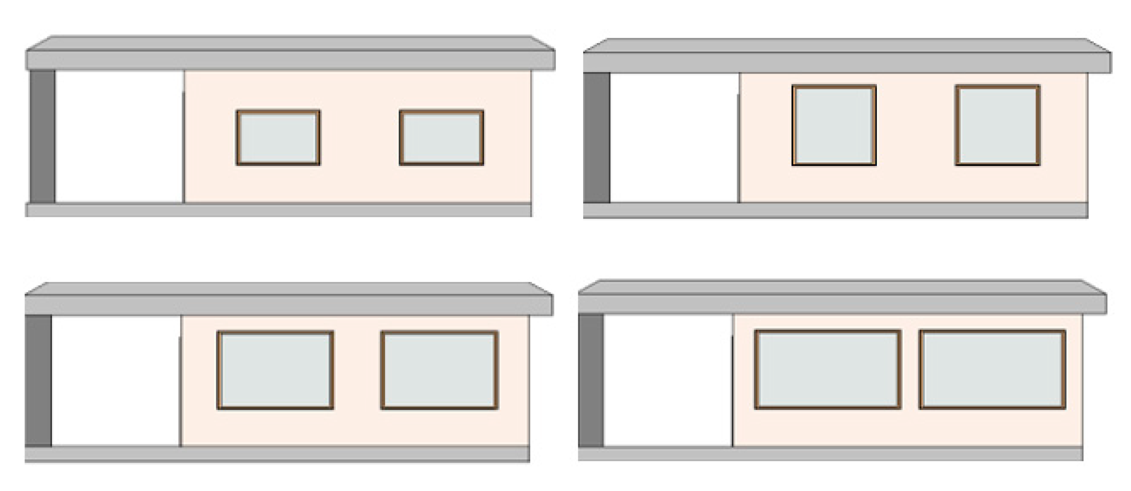
| A | 0.2 | 1900–2087.5 mm | 0.2 | 1525–1900 mm | 0.2 | 983–1150 mm | 0.2 | 750–1525 mm | Double Glazed Tint/Clear Air Fill/Aluminium |
| B | 0.2 | 750–1525 mm | 0.2 | 750–1525 mm | 0.2 | 750–775 mm | 0.4 | 750–1525 mm | Single Glazed Tint/Timber/uPVC/Fiberglass |
| C | 0.2 | 1900–2087.5 mm | 0.4 | 750–1525 mm | 0.2 | 750–775 mm | 0.4 | 750–1525 mm | Single Glazed Clear/Timber/uPVC/Fiberglass |
| D | 0.2 | 1900–2087.5 mm | 0.4 | 750–1525 mm | 0.2 | 775–983 mm | 0.4 | 750–1525 mm | Single Glazed Clear/Timber/uPVC/Fiberglass |
Publisher’s Note: MDPI stays neutral with regard to jurisdictional claims in published maps and institutional affiliations. |
© 2020 by the authors. Licensee MDPI, Basel, Switzerland. This article is an open access article distributed under the terms and conditions of the Creative Commons Attribution (CC BY) license (http://creativecommons.org/licenses/by/4.0/).
Share and Cite
Chen, Z.; Hammad, A.W.A.; Kamardeen, I.; Haddad, A. Optimising Window Design on Residential Building Facades by Considering Heat Transfer and Natural Lighting in Nontropical Regions of Australia. Buildings 2020, 10, 206. https://doi.org/10.3390/buildings10110206
Chen Z, Hammad AWA, Kamardeen I, Haddad A. Optimising Window Design on Residential Building Facades by Considering Heat Transfer and Natural Lighting in Nontropical Regions of Australia. Buildings. 2020; 10(11):206. https://doi.org/10.3390/buildings10110206
Chicago/Turabian StyleChen, Zixuan, Ahmed W. A. Hammad, Imriyas Kamardeen, and Assed Haddad. 2020. "Optimising Window Design on Residential Building Facades by Considering Heat Transfer and Natural Lighting in Nontropical Regions of Australia" Buildings 10, no. 11: 206. https://doi.org/10.3390/buildings10110206
APA StyleChen, Z., Hammad, A. W. A., Kamardeen, I., & Haddad, A. (2020). Optimising Window Design on Residential Building Facades by Considering Heat Transfer and Natural Lighting in Nontropical Regions of Australia. Buildings, 10(11), 206. https://doi.org/10.3390/buildings10110206