Abstract
With the constant expansion of the building sector as a major energy consumer in the modern world, the significance of energy-efficient building systems cannot be more emphasized. Most of the buildings are now equipped with an electric dashboard to record consumption data which presents a significant scope of research by utilizing those data in energy modeling. This paper investigates conventional regression modeling in building energy estimation and proposes three models with data classifications to improve their performance. The proposed models are regression models and an artificial neural network model with data classification for predicting hourly or sub-hourly energy usage in four different buildings. Energy data is collected from a building energy simulation program and existing buildings to develop the models for detailed analysis. Data classification is recommended according to the system operating schedules of the buildings and models are tested for their performance in capturing the data trends resulting from those schedules. Proposed regression models and an ANN model with the recommended classification show very accurate results in estimating energy demand compared to conventional regression models. Correlation coefficient and root mean squared error values improve noticeably for the proposed models and they can potentially be utilized for energy conservation purposes and energy savings in the buildings.
1. Introduction
The building sector consumes a large portion of primary energy in the United States which amounted to almost 40% in the year 2019 [1]. With the growth of population and constant expansion of the building sector, it has now become significant to explore strategies of energy conservation and the accurate forecast of building energy use with an aim to improve energy performance and reduce environmental impact [2,3]. However, energy consumption in buildings depends on many factors such as weather parameters, building characteristics, energy system design and control, schedules, as well as occupants’ behavior, [4], and therefore, the precise prediction of building energy usage is quite a complex task. A lot of recent studies have been dedicated to predicting energy consumption efficiency and efficiency with various strategies and techniques; either elaborate or simplified [2,5]. Among the approaches, computational modeling has been a viable technique that is used for the design and development of energy-efficient building systems [6].
Most of the buildings now have electric power meter dashboards to record the data on the electric energy consumption at specific intervals for the building. These data can easily be collected and depending on the available data, different computational modeling techniques can be used to estimate building energy consumption and many other smart applications like demand response, optimization, fault detection, and energy conservation [7,8,9]. However, the abundant data from these buildings are not always utilized effectively for energy estimation and conservation purposes due to the lack of appropriate computational means and accurate energy consumption assessment. This offers a significant scope of investigation on how the computational models can be built, developed, and applied precisely to the available data sets of a building for building energy estimation and energy-saving purposes.
According to the ASHRAE (American Society of Heating, Refrigerating and Air-Conditioning Engineers) handbook 2009 [10], computational modeling techniques can be broadly divided into two categories, a forward approach built on the detailed physical information of the system and a data-driven approach built on the acquired data to develop a mathematical description of the system [4,10]. Data-driven approaches can again be two types; a statistical approach and a machine learning approach. Statistical models have shown good performance in predicting medium to long-term energy consumption [5]. Among the statistical computational models, the single or multivariable regression models are more convenient and easier for applications in comparison to other models like HVAC system models [11], models which rely on detailed energy simulations [12] or Fourier series function [13,14]. In addition, the regression models require less computational power with a satisfactory forecast ability [15]. A major advantage of these models is that they can be easily automated and applied to a large number of buildings if utility billing data are available [10]. Therefore, a single or multivariate regression model has been applied in many instances for energy assessment and finding appropriate measures for a project [13,16]. Performances of different devices like pumps, chillers, and fans are also widely evaluated using regression models [17,18,19]. Prescreening against test regression models for energy conservation purposes has also been advantageous for many agencies [10].
Generally, regression models are built using outdoor dry bulb temperature and dew point temperature as the major regressors. Other environmental variables such as humidity, solar gain, etc., are often difficult to measure in actual buildings. Additionally, they may not change significantly over time. Therefore, they are not usually a good fit for regressor variables. Considering such limitations related to other variables, the outdoor temperature is recommended to be the most significant variable for all data-driven modeling techniques for predicting building energy consumption [6,10,14].
Regression models are relatively simple and easy to develop with appropriate regressor variables. However, they may fail to predict the data trends occurring due to the system operating schedules and other important factors such as the nonlinear patterns of the data [20]. Thus, regression models may require some modifications to reduce the error in forecasting building energy consumption with operating schedules and other factors.
Machine learning, on the other hand, is a branch of artificial intelligence where computers learn without being explicitly programmed to non-linearly transform data for a forecast [4,21]. ML approaches are comparatively easier in energy forecasting than physics-based approaches that rely on precise input information [2,22]. For existing buildings, the machine learning approach has provided more accurate energy assumptions with recorded time series data due to the complex interactions of the energy systems [5,23]. Machine learning models determine the connection between the input and output variables using the given data to establish the pattern of energy consumption [24]. Cleaning and providing good data sets without too many outliers and inconsistencies also enhance the prediction ability of these models [22]. Amongst the machine learning techniques, the artificial neural network model is one of the most significant approaches to date. Artificial neural network (ANN) models are a non-linear information processing technique that functions similarly to the neurons of the brain [5,25]. When natural neurons receive a signal strong enough through the synapses, the neuron is activated and sends the signal to other synapses; triggering other neurons. The strength of these neuron connections is known as adaptive weights. In the computational model, the strength of the input depends on the weight of the neuron. By adjusting these weights, the computation of neurons can be changed to produce necessary outputs for specific inputs. A predictive model based on a specific cluster of data is built by training the neural network with that set of data which will also minimize the error for the outcome of the model [26]. ANN models have been used in many types of research from creating a framework for energy consumption raw data forecasting [3] for estimating building heating demand including solar water heating systems [27,28], cooling load [29,30], energy consumption [31,32], short-term and long-term electricity consumption [33,34], predicting sub-level component consumption, the behavior of HVAC systems and optimization [35,36,37] and fault detection and diagnosis [38,39] for the last twenty years. ANN models have also been used in conjunction with BIM to reduce the deviation between predicted and actual energy consumption [40]. As these models can be trained with various data sets, they can solve the problem even with failure elements present in the neural network, and so ANN models can be implemented on any type of application. However, preparing the model with the training data set can be time-consuming, especially with larger networks and ANN models will not perform well outside their training range. Additionally, if there is too much noise in the data, the ANN model can start overfitting the data and the general trends will be lost in the prediction [5]. In such cases, some adjustments of the data are required for the ANN model to train and perform well.
In the ASHRAE handbook [10], simple to multivariate regression models are mentioned as simple models with a fast calculation time and have medium accuracy. On the other hand, artificial neural network models are complex to build but have a relatively faster calculation time with a high accuracy of results. Considering all the points, regression models and artificial neural network models are examined for four buildings in this paper to explore the aspects of computational modeling for hourly or sub-hourly energy consumptions. The major objective of this research is to investigate the performance of regression and ANN models for building energy estimation and energy savings. Two of the four buildings discussed here have the system operating schedules in place according to occupancy, time, and days of the week. As mentioned above, conventional regression models and ANN models may not be able to capture the specific data trends resulting from these schedules. Thus, data classification is proposed for the better performance of the models in predicting building energy consumption. Classifying the data for a better accuracy of models is an innovative step taken for this research, and this is a major contributor to model development. Here, three traditional single to multiple regression models, two proposed regression models, and an artificial neural network model including recommended classifications are discussed and compared using the correlation coefficient values for each of the models. The models are also compared with root mean squared error values to evaluate the accuracy of the performance. Electric energy consumption data from the whole building at 15 min intervals are collected from existing buildings and employed to build the models. In addition, a widely used energy simulation program is used with added hourly energy data for investigation and thorough analysis.
2. Methodology
2.1. Building Energy Data Collection and Operating Schedules
Four buildings are taken from different locations in the United States for the study of energy consumption. Among them, Buildings 3 and 4 are existing buildings located in Greensboro, NC. Sub-hourly energy consumption data are collected from these two actual buildings. The other two buildings (Buildings 1 and 2) are simulated using energy simulation software eQuest (eQuest Version 3.65) and the hourly energy consumption is derived from those simulations. All the buildings have a similar area within the range of 40,000–60,000 ft2 (3716.1–5574.2 m2) and are equipped with chilled water VAV (Variable Air Volume) systems. However, the buildings have different operating schedules. Building 1 consisting of classes and offices has an occupancy schedule of 100% from 7 a.m. to 10 p.m. on weekdays and 50% occupied from 8 a.m. to 8 p.m. on weekends. The heating and cooling setback temperatures are set at 82 and 62 °F (27.8 and 16.7 °C). Buildings 2 is an office building where the mechanical system starts at 7 a.m. and stops at 6 p.m. These two systems run with a 100% occupancy schedule from 8 a.m. to 5 p.m. on weekdays and they stay completely off during weekends. No schedules were in place for Buildings 3 and 4 consisting of offices and classes during the data collection.
2.2. Building Energy Estimation Models
This study explores the techniques to estimate hourly or sub-hourly energy usage by utilizing data classifications in regression models and artificial neural networks based on various operating schedules. As one model cannot be applied suitably for all applications, six different models are investigated, among which the first three are conventional techniques appropriate for most M&V (Measurement and Verification) applications, and the last three are proposed with the consideration of different operating schedules and other factors in energy consumption.
2.3. Conventional Regression Models
Model 1 is a simple weather-based model with two regression parameters a and b and one regressor variable ta which is the dry-bulb temperature. Model 2 is a single variant change point model where the dry bulb temperature ta is the only regressor variable, but it has a specific change point temperature t1 (for example 55 °F). The equations for single variant Models 1 and 2 are given below with one regressor and two parameters. Model 3 is a multivariate model that works similarly like Model 1 with a second regressor outdoor air dew point temperature noted as tp. The equation for Model 3 with multiple variables is also given below. If the monthly consumption (utility bill) data and average temperatures are available for a building, these three models can be easily applied, whether it is a commercial building or a residential. Nevertheless, these models may not perform well in terms of hourly or sub-hourly consumption when considering the building schedules:
Y = a + b·ta
Y = a + b·(ta − t1)
Y = a + b·ta + c·tdp
2.4. Data Classification and Proposed Models
To deal with the inaccuracy in terms of hourly and sub-hourly energy consumption from the first three models, Models 4, 5, and 6 are proposed. For the model development, the whole one-year data collected were first made into two data sets which consisted of three months and nine months. The models are then trained with data sets and then tested against the testing data set to the actual energy demand. Best fitting results for training and testing data sets are selected for each model for the buildings. For the data classification, the available data are classified according to the building schedules such as occupied or unoccupied, weekdays or weekends, and other aspects that vary according to the operating schedules of the system. One class of data is for the occupied hours in the buildings according to the schedules and types of buildings where energy demands are high. The second data class is the unoccupied period in the buildings where the system is running in early or late hours with lower energy demand. The third class of data is for weekends and holidays where the energy consumption is either low or the system is completely switched off according to different building schedules. Figure 1 shows the methodology for proposed Models 4, 5, and 6.
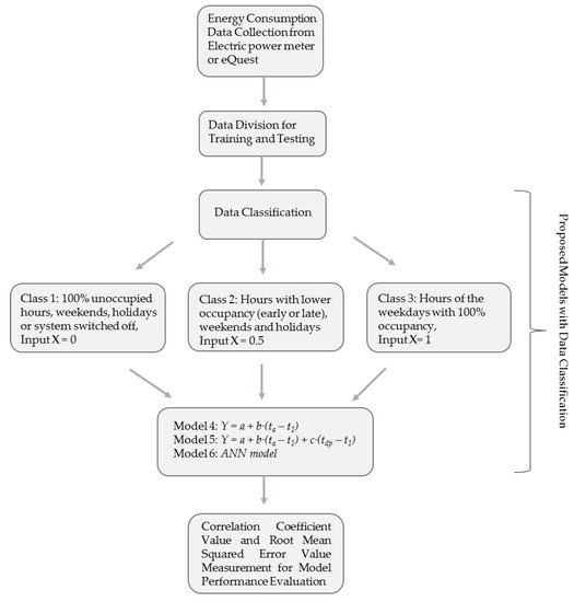
Figure 1.
Flowchart for the methodology of proposed models.
After classifying the data, the proposed models are investigated for performance. Here, for Model 4, each data cluster is put into the single variant model with a change-point temperature. Model 5 works similarly as Model 4 with an addition of the second regressor outdoor dew point temperature.
In addition to these regression models, Model 6 is also proposed and investigated which is an artificial neural network model. It comprises outdoor air temperature, dew point temperature, and class numbers like 1,2, and 3 as inputs. For the ANN model, it was first optimized for a specific number of neurons as this is an important factor in performance accuracy. The optimum number of neurons may vary according to the available data sets used to develop the model. The ANN model will show higher accuracy and performance in one criterion for some numbers of neurons, while not performing similarly for another number of neurons. Thus, the model is first run with numbers of neurons ranging from 5 to 200 to identify the optimum number A specific number of neurons is then selected for the ANN model according to the results in terms of correlation coefficient values. After optimizing the ANN model, it was trained and tested using Matlab Artificial Neural Network (MathWorks R2020). Data classification is then applied with the ANN model to improve the performance of the model.
2.5. Measurement of Correlation Coefficient r Values
The performance of the models is evaluated by comparing their correlation coefficient r values. For further evaluation, three other locations were selected for Buildings 1 and 2, and the data are collected from the simulation. The r values from the other locations were also compared to assess the performances of the conventional and proposed models. The correlation coefficient r-value in a data series is a measurement of how close the data in a plot fall along the straight line. If the value is closer to 1, the data are considered better in the equation. Data sets close to 0 show a negligible relationship with the straight line. Correlation coefficient values are usually calculated with statistical tools due to the lengthy calculation [41]. In this paper, r values are calculated and compared for training and testing data sets of each model.
2.6. Measurement of Root Mean Squared Error Values
The models were further assessed with the root mean squared error values to compare the prediction errors. Root mean squared error or RMSE is the standard deviation of residual or prediction errors [42]. Residuals are a measurement of the distances of data points from the regression line; RMSE values show how concentrated or spread out the residuals are. So, a higher RMSE value denotes more spread out residuals; which implies the poor performance of the model. RMSE values were calculated from mean squared error values for each model for Greensboro, NC location. The equations for mean squared error and RMSE are given below:
where:
e = error
n = data sample
3. Results
3.1. Energy Consumption of the Buildings and Data Trends
Electric energy consumptions for those four buildings are shown below in Figure 2 with respect to outside dry bulb temperature. In the figure, all the buildings are in Greensboro, NC. Different trends of data can be observed for these buildings due to the operating schedules in place and applied data classification according to those schedules. Data from Building 1 shows two different trends for the full occupied period and unoccupied period; whereas the data from Building 2 shows three trends of the occupied period, unoccupied period, and HVAC systems shut off period to the outside temperature. However, as Buildings 3 and 4 have no operating schedules, energy demand is higher even with the lower outside temperature.
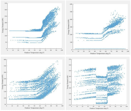
Figure 2.
Energy consumption in Buildings 1 and 2 (above), Buildings 3 and 4 (below) with respect to outdoor dry bulb temperature in Greensboro, NC.
For data classification in Building 1, the building was occupied from 7 a.m. to 10 p.m. on weekdays and from 8 a.m. to 8 p.m. on weekends. The system was running all-time with low occupancy at 6 a.m. and 10 p.m. and no occupancy from 1–4 a.m. and from 11 p.m. to 12 a.m. In the case of Building 2, the system was running from 8 a.m. to 5 p.m. with an early start at 7 a.m. and late shut down at 6 p.m. The system was kept off from hours 1–6 a.m., 6 p.m. to 12 a.m. on weekdays, and all hours during weekends or holidays. For Building 3, the system was operating with full occupancy from 9 a.m. to 5 p.m., lower occupancy during the hours 7–8 a.m., 6–10 p.m., and zero occupancies from 1–6 a.m. and from 11 p.m. to 12 a.m. Building 4 was classified as the system running from 7 a.m. to 7 p.m. with full occupancy, from 5–6 a.m. and from 8 p.m.–12 a.m. with lower occupancy, and from 1–4 a.m. with zero occupancies. As Buildings 3 and 4 had no schedules in place, they were considered half occupied during weekends and holidays, with the system always running. As shown in Figure 2, energy demand with outside dry bulb temperature shows various data clusters for each building with only Building 2 having zero demand data cluster due to the system being off according to the aforementioned schedules.
3.2. Training and Testing Data Sets for Models
All the models were trained with training data sets after data classification and then tested against the testing data sets. The best performing sets of both were then taken to evaluate the performance of the model. Figure 3 and Figure 4 are the best fitting results for Models 3, 4, 5, and 6 for Buildings 1 and 2 for Greensboro, NC. It was observed that the training and testing data sets for Models 1 and 2 were not close or following a similar path to the straight line in Figure 3. These two models were omitted from the figure for this reason. Model 3 has a similar path, although the points are dispersed all over the area. As it is seen from the figure, Model 3 shows the least accuracy in the simulations of energy demand, while the proposed models; Models 4 and 5 perform satisfactorily in terms of simulating the energy demand for Building 1 with operating schedules.
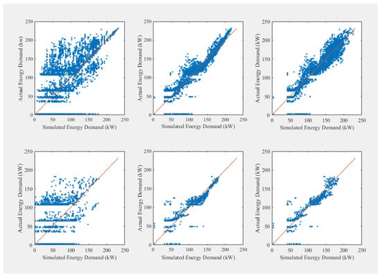
Figure 3.
Training (above) and testing (below) data for the performance of Models 3,4, and 5 for Building 1.
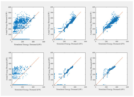
Figure 4.
Training (above) and testing (below) data for the performance of Models 3,4, and 5 for Building 2.
3.3. Optimization of ANN Model
The artificial neural network model with data classifications was used for all the buildings. First, the model was run several times with a varying number of neurons to obtain the optimum number of neurons. The varying range was from 5 to 200 neurons. It was observed that between 10 neurons to 100 neurons, the r-value did not change abruptly for both buildings. Additionally, as seen in Figure 5, for larger numbers with more than 100 neurons, the testing data results do not improve. To save time in running the model, neuron numbers larger than 200 were not tested. Thus, 100 neurons are taken as the optimum number. In this case, the ANN model consists of 100 neurons with one hidden layer, one output layer with one neuron, and an activation function. Care should be taken in selecting the number of neurons as a random number of neurons may not perform very well in the case of ANN producing poor results for the testing data set. Then, the model was run for all the buildings which show better r values than Model 5 for all the buildings. Figure 6 shows the performance of ANN model for all four buildings in Greensboro, NC.
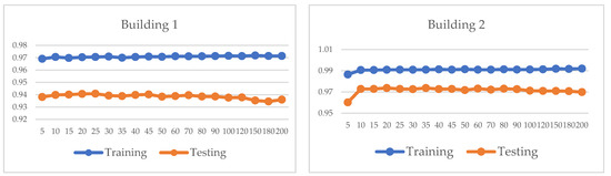
Figure 5.
ANN model optimization for neuron numbers.
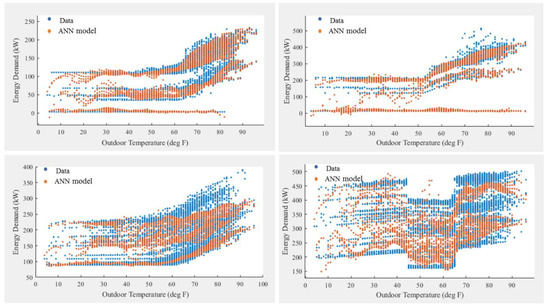
Figure 6.
Performance of ANN model for Buildings 1 and 2 (above), Buildings 3 and 4 (below).
3.4. Evaluation of Correlation Coefficient r Values
The six models described in Section 2 were then tested on the four buildings. Buildings 1 and 2 were selected to visualize the performance of each model in different locations. The correlation coefficient r values for each model are calculated and shown in Figure 7 for the training and testing data sets for four locations. As seen in Figure 7, Models 1, 2, and 3 which are the conventional regression models produce poor results for these buildings due to the presence of various data trends of the building energy consumption. By introducing change point temperature in Model 2, small improvements can be obtained in the values but not significant. Model 3 output data become even more dispersed although adding the second regressor makes the model comparatively better. On the other hand, proposed Models 4, 5, and 6 seemed to perform a lot better with high r values as the data for the buildings are divided into clusters. For instance, Model 4 has significantly higher r values than Model 2. Model 5 also shows improvements compared to Model 3. Model 6, which is the artificial neural network model, was observed to have the highest r-value for the training and testing data sets for both buildings in all locations.
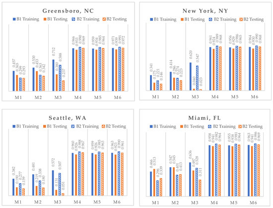
Figure 7.
Correlation coefficient values for training and testing data sets of six models in four different locations for Buildings 1 and 2.
Figure 8 shows how the models performed for the two actual buildings located in Greensboro, NC. Here, it is again observed that the proposed three models tend to perform better than the conventional regression models. Building 3 has an overall higher r value than Building 4. The proposed ANN model performed slightly better than other models for these two buildings as well.
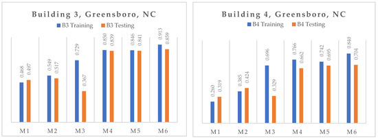
Figure 8.
Correlation coefficient values for the training and testing data sets of six models for existing Buildings 3 and 4.
3.5. Evaluation of RMSE Values
Figure 9 presents how each model performs in terms of average RMSE values for all four buildings. Here, n (data sample) was taken as the whole year data sample including training and testing sample sets to calculate the mean squared errors first. Then RMSE values were from the MSE values for each building. As it is seen in the figure, RMSE values show a trend where Models 1, 2, and 3 have higher numbers and proposed models show lower numbers. This indicated that the proposed models have a lower sum of errors and they perform better than the conventional regression models. For Buildings 1 and 2, the difference between the RMSE values in terms of conventional and proposed models are significantly high. Building 4 has an overall higher RMSE value for all the models, yet the better performance of the proposed regression and ANN models are distinguishable.
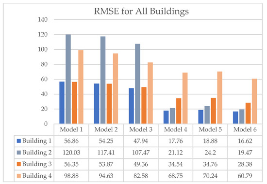
Figure 9.
Average RMSE values for all buildings in Greensboro, NC.
3.6. Performance of All Models
Figure 10 shows how each model performs for Building 1 in terms of predicting the energy demand with respect to the outdoor temperature. As the system operation schedules are not taken into consideration for the first three models, the performance was far from accurate for hourly and sub-hourly consumptions. The trend lines and data points were dispersed for these models. However, these models may be able to forecast daily average or monthly consumptions accurately to a certain degree. On the other hand, the proposed models with data classification seem to perform better in terms of predicting hourly or sub-hourly energy consumptions. The data points and trend lines are very consistent with the energy demand for different operating schedules.
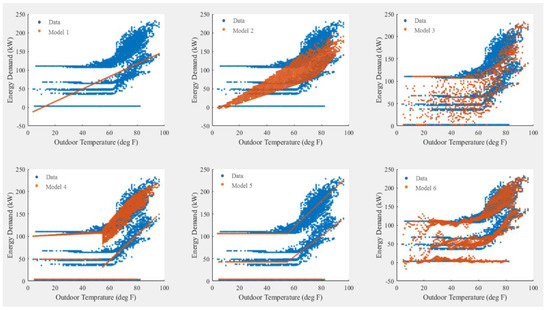
Figure 10.
Prediction performance of all models for Building 1.
4. Conclusions and Future Work
Energy conservation has become a vital concern in the modern world. Computational modeling techniques can be used to predict the energy consumption of a new building or existing one to employ appropriate measures and systems for energy conservation. In this paper, six different data-based models were tested on four buildings to estimate hourly and sub-hourly energy consumptions. It was observed that simplified regression models did not perform well enough to predict energy demand when the system has operating schedules. To deal with the inaccuracy, data classification is proposed according to occupancy, day of the week, and hours. Classifying the data for regression and artificial neural models has proven to be effective for better model performance. All the regression models and artificial neural network model are then evaluated with the building energy consumption data. Two different indicators were used to evaluate the performance of all six models—coefficient correlation values and root mean squared errors. In both cases, introducing data classification has shown significant improvement in performance for the regression models. Proposed Models 4 and 5 showed significantly better results for training and testing data in terms of correlation coefficient values. They also have much lower average RMSE values than the first three models which further validates the efficiency of the proposed models. The ANN model with data classification was tested with an optimal number of neurons, which is an unorthodox proposition in this research These models have r values very close to 1 for Buildings 1 and 2 in different weather locations, existing Buildings 3 and 4 also have higher r values for proposed models compared to conventional regression models. The proposed ANN model has significantly low RMSE values for Buildings 1, 2, and 3. Even though Building 4 has higher RMSE values than other buildings, the RMSE values for proposed models show better performance than the first three conventional models for all buildings. The proposed regression models and ANN model with recommended classifications have performed with certain accuracy in terms of predicting energy demand for the buildings, especially hourly and sub-hourly consumptions.
Predicting energy demand and applying energy-efficient systems using regression models and ANN models with data classification in the design stage of new buildings lie in the future scope of this work. These models can be easily applied to a large number of existing buildings with available utility billing data for energy demand estimation, long-term prediction to improve energy consumption, and can potentially make contributions towards energy conservation measures which will serve a broader research domain.
Author Contributions
Conceptualization, I.R. and N.N.; methodology, I.R. and N.N.; software, I.R. and N.N.;formal analysis, I.R. and N.N.; investigation, I.R. and N.N.; resources, I.R. and N.N.; data curation, I.R. and N.N.; writing—original draft preparation, I.R.; writing—review and editing, I.R.; final draft revision, I.R., N.N. and W.C.; visualization, I.R. and N.N.; supervision, N.N.; project administration, N.N. and W.C.; funding acquisition, N.N. and W.C. All authors have read and agreed to the published version of the manuscript.
Funding
This work is partially supported by the Korea Agency for Infrastructure Technology Advancement (KAIA) grant funded by the Ministry of Land, Infrastructure, and Transport (20AUDPB099686-06).
Conflicts of Interest
The authors declare no conflict of interest. The funders had no role in the design of the study; in the collection, analyses, or interpretation of data; in the writing of the manuscript, or in the decision to publish the results.
References
- EIA. Consumption & Efficiency—U.S. Energy Information Administration. Available online: https://www.eia.gov/consumption/index.php (accessed on 8 July 2020).
- Zhao, H.; Magoulès, F. A review on the prediction of building energy consumption. Renew. Sustain. Energy Rev. 2012, 16, 3586–3592. [Google Scholar] [CrossRef]
- Yang, J.; Tan, K.K.; Santamouris, M.; Lee, S.E. Building energy consumption raw data forecasting using data cleaning and deep recurrent neural networks. Buildings 2019, 9, 204. [Google Scholar] [CrossRef]
- Fumo, N. A review on the basics of building energy estimation. Renew. Sustain. Energy Rev. 2014, 31, 53–60. [Google Scholar] [CrossRef]
- Runge, J.; Zmeureanu, R. Forecasting energy use in buildings using artificial neural networks: A review. Energies 2019, 12, 3254. [Google Scholar] [CrossRef]
- Lam, J.C.; Wan, K.K.W.; Liu, D.; Tsang, C.L. Multiple regression models for energy use in air-conditioned office buildings in different climates. Energy Convers. Manag. 2010, 51, 2692–2697. [Google Scholar] [CrossRef]
- ASHRAE. ASHRAE Handbook-Applications; American Society of Heating Refrigeration and Air Conditioning Engineers Inc.: Atlanta, GA, USA, 2015; Chapter 41. [Google Scholar]
- Nassif, N. Modeling and optimization of HVAC systems using artificial neural network and genetic algorithm. Build. Simul. 2013, 7, 237–245. [Google Scholar] [CrossRef]
- Seem, J.E. Using intelligent data analysis to detect abnormal energy consumption in buildings. Energy Build. 2007, 39, 52–58. [Google Scholar] [CrossRef]
- ASHRAE. ASHRAE Handbook—Energy Estimating and Modeling Methods; American Society of Heating Refrigeration and Air Conditioning Engineers Inc.: Atlanta, GA, USA, 2009; Chapter 19. [Google Scholar]
- Katipamula, S.; Claridge, D.E. Use of simplified system models to measure retrofit energy savings. J. Sol. Energy Eng. 1993, 115, 57–68. [Google Scholar] [CrossRef]
- ASHRAE. ASHRAE Handbook—Fundamentals; American Society of Heating Refrigeration and Air Conditioning Engineers Inc.: Atlanta, GA, USA, 2013; Chapter 19. [Google Scholar]
- Ji, Y.; Xu, P.; Ye, Y. HVAC terminal hourly end-use disaggregation in commercial buildings with Fourier series model. Energy Build. 2015, 97, 33–46. [Google Scholar] [CrossRef]
- Dhar, A.; Reddy, T.; Claridge, D. Modeling hourly energy use in commercial buildings with Fourier series functional forms. J. Sol. Energy Eng. 1998, 120, 217–223. [Google Scholar] [CrossRef]
- Fumo, N.; Rafe Biswas, M.A. Regression analysis for prediction of residential energy consumption. Renew. Sustain. Energy Rev. 2015, 47, 332–343. [Google Scholar] [CrossRef]
- Nassif, N. Single and multivariate regression models for estimating monthly energy consumption in schools in hot and humid climates. Energy Eng. 2013, 110, 33–54. [Google Scholar] [CrossRef]
- Korolija, I.; Zhang, Y.; Marjanovic-Halburd, L.; Hanby, V.I. Regression models for predicting UK office building energy consumption from heating and cooling demands. Energy Build. 2013, 59, 214–227. [Google Scholar] [CrossRef]
- Stein, J.; Hydeman, M.M. Development and testing of the characteristic curve fan model. ASHRAE Trans. 2004, 110, 347–356. [Google Scholar]
- Hydeman, M.; Webb, N.; Sreedharan, P.; Blanc, S. Development and testing of a reformulated regression-based electric chiller model. ASHRAE Trans. 2002, 108, 1118–1127. [Google Scholar]
- Mat Daut, M.A.; Hassan, M.Y.; Abdullah, H.; Rahman, H.A.; Abdullah, M.P.; Hussin, F. Building electrical energy consumption forecasting analysis using conventional and artificial intelligence methods: A review. Renew. Sustain. Energy Rev. 2017, 70, 1108–1118. [Google Scholar] [CrossRef]
- Chakraborty, D.; Elzarka, H. Advanced machine learning techniques for building performance simulation: A comparative analysis. J. Build. Perform. Simul. 2019, 12, 193–207. [Google Scholar] [CrossRef]
- Mohammadiziazi, R.; Bilec, M.M. Application of machine learning for predicting building energy use at different temporal and spatial resolution under climate change in USA. Buildings 2020, 10, 139. [Google Scholar] [CrossRef]
- Deb, C.; Zhang, F.; Yang, J.; Lee, S.E.; Shah, K.W. A review on time series forecasting techniques for building energy consumption. Renew. Sustain. Energy Rev. 2017, 74, 902–924. [Google Scholar] [CrossRef]
- Seyedzadeh, S.; Rahimian, F.P.; Glesk, I.; Roper, M. Machine learning for estimation of building energy consumption and performance: A review. Vis. Eng. 2018, 6, 5. [Google Scholar] [CrossRef]
- Foucquier, A.; Robert, S.; Suard, F.; Stéphan, L.; Jay, A. State of the art in building modeling and energy performance prediction: A review. Renew. Sustain. Energy Rev. 2013, 23, 272–288. [Google Scholar] [CrossRef]
- Nassif, N.; Arida, M.; Talib, R. Development and testing of building energy model using non-linear auto regression neural networks. In Proceedings of the ASHRAE Annual Conference, St Louis, MO, USA, 25–29 June 2016. [Google Scholar]
- Ekici, B.B.; Aksoy, U.T. Prediction of building energy consumption by using artificial neural networks. Adv. Eng. Softw. 2009, 40, 356–362. [Google Scholar] [CrossRef]
- Kalogirou, S.A. Artificial neural networks in energy applications in buildings. Int. J. Low-Carbon Technol. 2006, 1, 201–216. [Google Scholar] [CrossRef]
- Alam, A.G.; Baek, C.I.; Han, H. Prediction and analysis of building energy efficiency using artificial neural network and design of experiments. Appl. Mech. Mater. 2016, 819, 541–545. [Google Scholar] [CrossRef]
- Yokoyama, R.; Wakui, T.; Satake, R. Prediction of energy demands using neural network with model identification by global optimization. Energy Convers. Manag. 2009, 50, 319–327. [Google Scholar] [CrossRef]
- Ferlito, S.; Atrigna, M.; Graditi, G.; De Vito, S.; Salvato, M.; Buonanno, A.; Di Francia, G. Predictive models for building’s energy consumption: An artificial neural network (ANN) approach. In Proceedings of the 2015 XVIII Aisem Annual Conference, Trento, Italy, 3–5 February 2015; pp. 1–4. [Google Scholar]
- Hong, S.M.; Paterson, G.; Mumovic, D.; Steadman, P. Improved benchmarking comparability for energy consumption in schools. Build. Res. Inf. 2014, 42, 47–61. [Google Scholar] [CrossRef]
- Mena, R.; Rodríguez, F.; Castilla, M.; Arahal, M. A prediction model based on neural networks for the energy consumption of a bioclimatic building. Energy Build. 2014, 82, 142–155. [Google Scholar] [CrossRef]
- Azadeh, A.; Ghaderi, S.F.; Sohrabkhani, S. Annual electricity consumption forecasting by neural network in high energy-consuming industrial sectors. Energy Convers. Manag. 2008, 49, 2272–2278. [Google Scholar] [CrossRef]
- Hou, Z.; Lian, Z.; Yao, Y.; Yuan, X. Cooling-load prediction by the combination of rough set theory and an artificial neural-network-based on data-fusion technique. Appl. Energy 2006, 83, 1033–1046. [Google Scholar] [CrossRef]
- Ben-Nakhi, A.; Mahmoud, M. Energy conservation in buildings through efficient A/C control using neural networks. Appl. Energy 2002, 73, 5–23. [Google Scholar] [CrossRef]
- Nassif, N. Regression and artificial neural network models with data classifications for building energy predictions. ASHRAE Trans. 2018, 124, 52–60. [Google Scholar]
- Magoulès, F.; Zhao, H.; Elizondo, D. Development of an RDP neural network for building energy consumption fault detection and diagnosis. Energy Build. 2013, 62, 133–138. [Google Scholar] [CrossRef]
- Lee, W.Y.; House, J.M.; Kyong, N.H. Subsystem level fault diagnosis of a building’s air-handling unit using general regression neural networks. Appl. Energy 2004, 77, 153–170. [Google Scholar] [CrossRef]
- Hammad, A.W. Minimising the deviation between predicted and actual building performance via use of neural networks and BIM. Buildings 2019, 9, 131. [Google Scholar] [CrossRef]
- Taylor, C. How to Calculate the Correlation Coefficient. Thought Co. 28 January 2020. Available online: https://www.thoughtco.com/how-to-calculate-the-correlation-coefficient-3126228 (accessed on 9 August 2020).
- Stephanie, G. RMSE: Root Mean Square Error. Statistics How To. Available online: https://www.statisticshowto.com/probability-and-statistics/regression-analysis/rmse-root-mean-square-error/ (accessed on 17 October 2020).
Publisher’s Note: MDPI stays neutral with regard to jurisdictional claims in published maps and institutional affiliations. |
© 2020 by the authors. Licensee MDPI, Basel, Switzerland. This article is an open access article distributed under the terms and conditions of the Creative Commons Attribution (CC BY) license (http://creativecommons.org/licenses/by/4.0/).