1. Introduction
The optimal control of heating, ventilation, and air-conditioning (HVAC) systems in buildings can save a substantial amount of energy. Many variables can be controlled in buildings to achieve energy savings and operating an HVAC system with the optimal control variables within the operating conditions of the system is critical for saving energy and improving the system’s overall performance and efficiency. Researchers have conducted numerous studies in attempts to achieve such optimal control. The effectiveness of several typical control methods of HVAC systems has been demonstrated in a number of studies; these methods include near-optimal control [
1], the ‘proportional integrated derivative’ approach [
2,
3], and model predictive control [
4,
5,
6]. Recently, as the amount of data and information that can be obtained from buildings has increased significantly and the computational performance of computers has improved, researchers have actively employed artificial intelligence or machine learning techniques to optimize and control HVAC systems [
7,
8,
9]. Among the machine learning techniques, genetic algorithms (GAs) are known to be suitable in complex conditions, such as large amounts of data and parameters, and are especially suitable for the optimization of HVAC systems in buildings [
10,
11].
In previous work, the authors conducted studies of optimal HVAC control methods using GAs that were applied to both a variable air volume (VAV) air-conditioning system and chilled water system to optimize the control variables in each system [
12,
13]. Two control variables for each system were analyzed in terms of time units, and the energy savings of the entire system for the cooling period were compared with the energy savings per component. Although the VAV air conditioning system and the chilled water system were divided into separate systems because they are composed of separate loops, the subsystem concept of an HVAC system affects its performance at the system level. So, with regard to the entire HVAC system, changes in the control variables and energy savings rates can show different characteristics according to changes in the setting or number of the control points.
The study of optimization using GAs is suitable for optimization of the complex composition of building and HVAC systems, and has already been verified in previous studies [
9,
12,
13,
14,
15].
However, it has not yet been resolved whether the combination of the location or number of control points among the multiple control variables is more efficient when optimizing using GAs. When applying control to buildings, it is also very important to provide appropriate adjustment of control variables, and it is necessary to apply a control scenario in many cases and compare the effects of control. Based on the results of this study, a guide can be provided for selecting each effective combination of control variables and an adjustment within the HVAC system.
As a follow-up to our earlier studies [
12,
13], the main purpose of this study was to compare the characteristics of different optimal control methods by combining the two methods (air-side and water-side) with additional control variables in an HVAC system’s controllable points during cooling periods and organizing the control scenarios by setting and variables of the control points in the HVAC system. The method for deriving the optimal control variables for an HVAC system uses a GA in the same way as in the previous studies [
12,
13]. The main control variables in a ‘combined’ HVAC system that consists of both a VAV system and a chilled water loop are the supply air temperature, duct static pressure, chilled water supply temperature, and pump differential pressure, all of which are controlled simultaneously for the proposed optimization. After constructing three optimal control scenarios according to the setting and type and number of control variables, we compared the changes in the control variables and the energy savings percentages during the cooling season for each control scenario.
2. Building Model and HVAC System Description
2.1. Data Generation
In order to derive the optimal control variables to save energy for an HVAC system using a GA, several input data for driving the optimization algorithm are required. In this study, a reference building proposed by the United States Department of Energy’s Building Energy Codes Program [
16] and ASHRAE (American Society of Heating, Refrigerating and Air-Conditioning Engineers) Standard 90.1 [
17] were simulated using EnergyPlus 8.9.0 to evaluate the model building’s energy performance. Among the choice of reference buildings, we selected the Large Office Building [
18,
19,
20] of Commercial Prototype Building Models. The location of the building, weather data, internal heating, and operation schedule of the facility system all can be used to predict the airflow supply in the building. These variables were changed under the same conditions and used in a prior study to fit a domestic situation [
12], energy consumption prediction [
19], and optimization of a VAV system [
12].
Table 1 summarizes the major information and simulation conditions of the reference building used also in the current study.
The human factor, such as the number of occupants and behavior [
21,
22], should be considered important because of its huge impact on the energy performance of buildings. In this study, the suggested typical occupancy schedule and metabolic rate in the ASHRAE model were used.
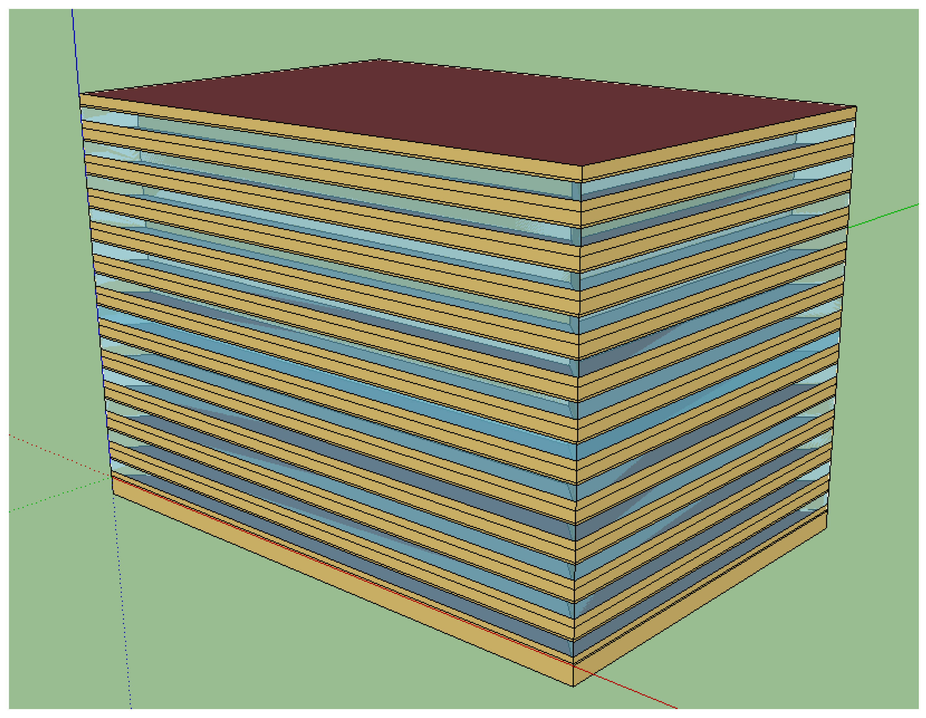
The reference building is divided into 19 zones, of which conditioned zones are 15 zones excluding basements and plenums. All conditioned zones are the same set point.
Figure 1 shows a 3D view of the reference building used in this study.
The weather data were converted from the test reference year (TRY) format in Seoul to the EnergyPlus Weather (EPW) file format; the time-step used to generate the data was one hour. The simulation period for the reference building was 2928 h of data from May to September.
2.2. HVAC Systems and Control Set Points
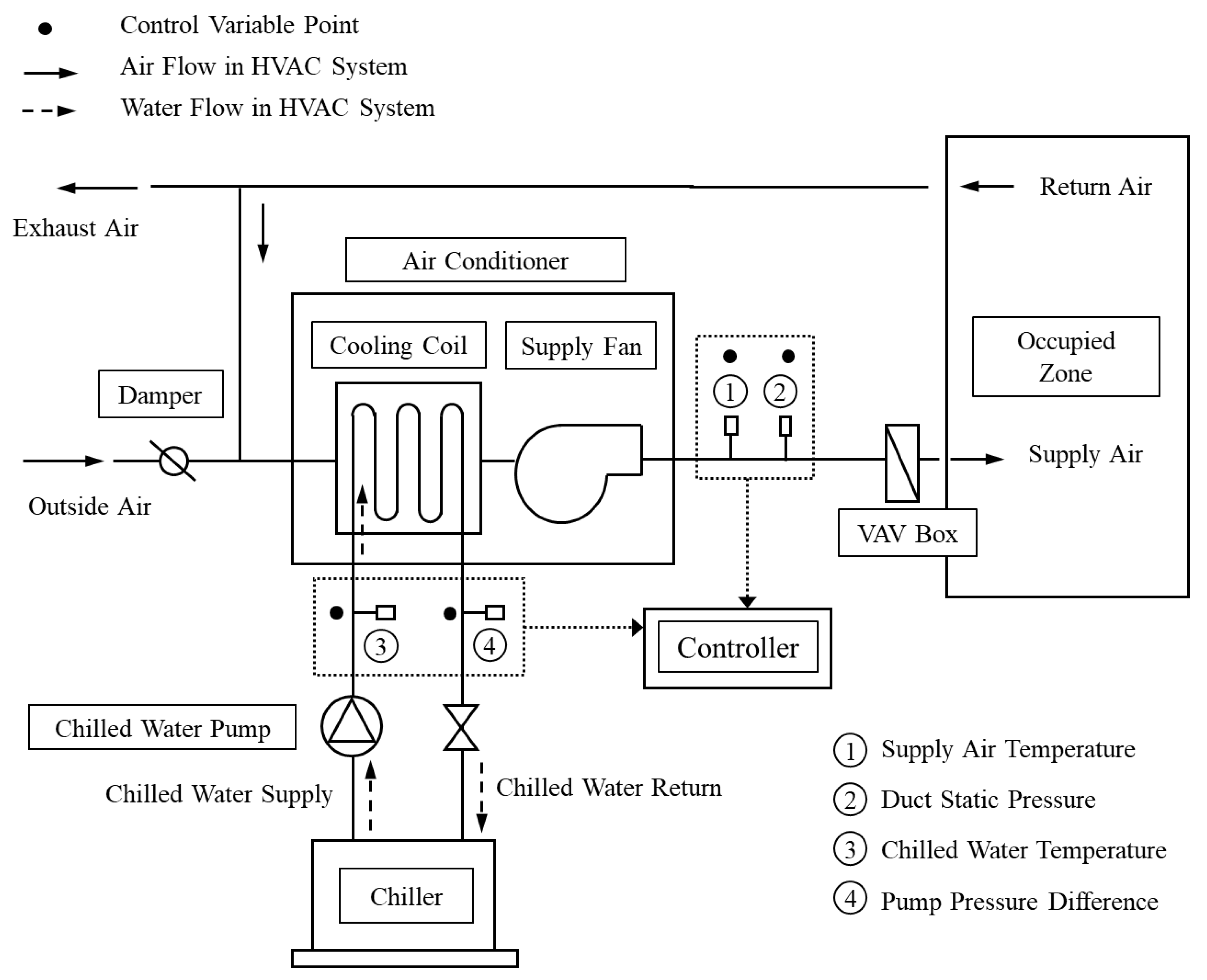
The HVAC system of the standard building modeled in this study cools each zone using a VAV system. The HVAC system consists of a fan, an air handling unit (AHU), a chiller, and a chilled water pump. In order to improve the building’s energy efficiency by optimizing the HVAC system, many control variables at the system level can be considered. However, in this study, given the HVAC system that is configured in the target building, the ‘air-side’ variables, which include the VAV system, the supply air temperature, and the duct static pressure, were selected as the control target. The ‘water-side’ variables, which include the chilled water system, utilize the chilled water temperature and pump pressure difference as the control variable settings.
Figure 2 presents a schematic diagram of the control set points for the supply air temperature, duct static pressure, chilled water temperature, and pump pressure difference that were selected as the control set points in this study and the configuration of the HVAC system. In the HVAC system, the fan efficiency was 0.6, the pump efficiency was 0.9, and there is no heat loss in ducts and pipes, and insulation is assumed to be adiabatic.
3. Genetic Algorithm-Based Optimal Control Variable Calculations and Optimal Control Scenario Composition
3.1. Determination of Genetic Algorithm-Based Optimal Control Variables
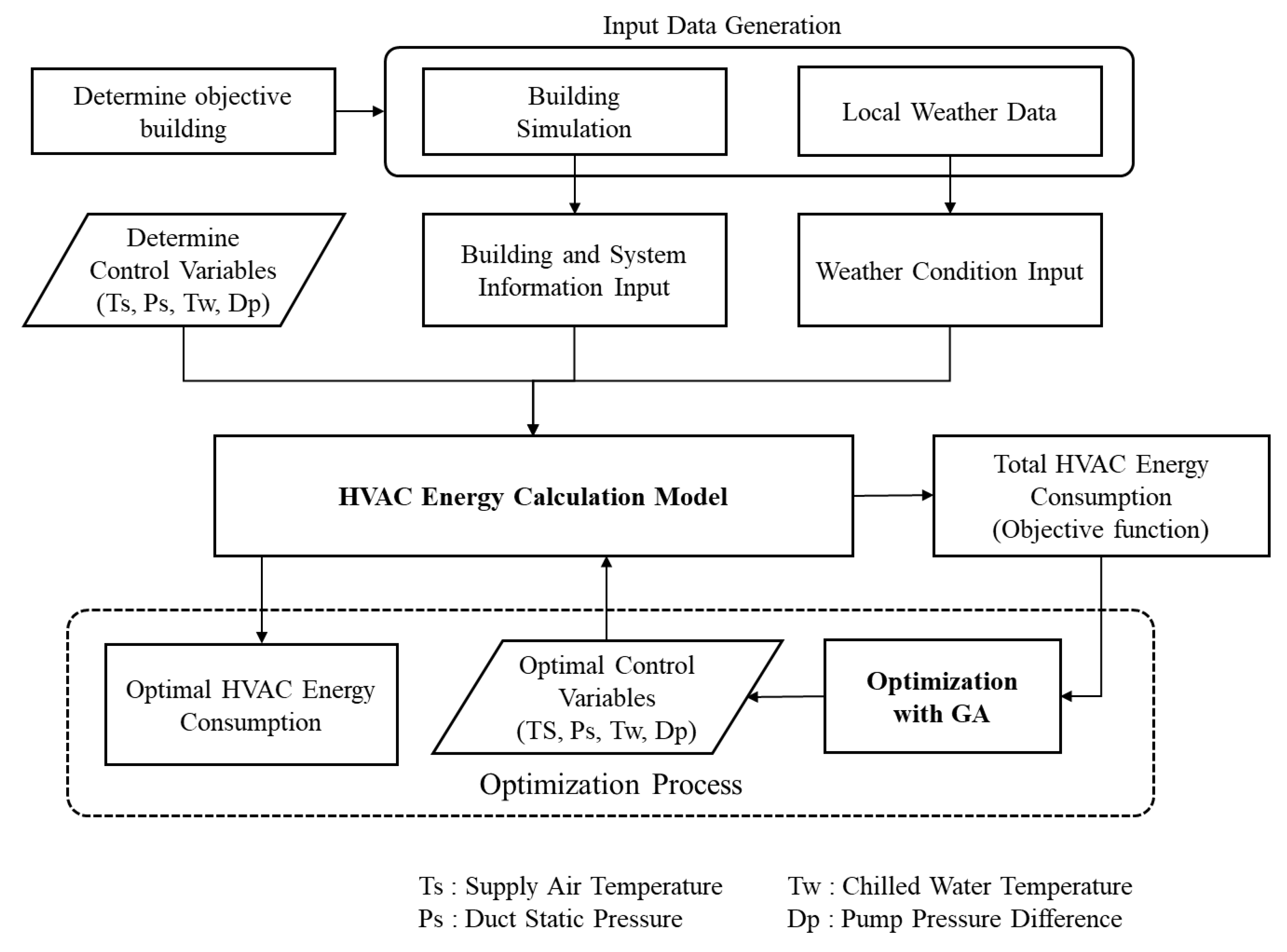
In this study, we used a GA to determine the optimal control of the HVAC system. The objective function of the GA is the sum of the total energy consumption of the HVAC system. When optimization is performed after setting the required number of populations and the selection range of the solution in the GA, the algorithm calculates the optimized control value when the total energy consumption of the system becomes the minimum. The computation of the GA prevents the repetition of unnecessary computations and allows the computation to be performed up to 100 generations with consideration of the proper computation time. The optimal control variables were calculated in units of one hour, and then each calculated optimal control variable was updated to a real-time input value for the control of the HVAC system in order to perform an optimal control operation.
Figure 3 is a flowchart of the process of calculating the real-time optimal control variables and the process of the optimal control operation method.
In the process of calculating the optimal control variables for the optimal control operation, we used a mathematical model from the literature [
12,
23,
24] to calculate the energy consumption of the HVAC system. Among the input values required for the calculations, the main values used as fixed variables were the simulation output values of the reference building. The model used to calculate the energy consumption of each component in the HVAC system was programmed using MATLAB R2018a, and the GA for optimization was programmed using MATLAB’s Global Optimization Toolbox.
3.2. Genetic Algorithm Calculation and Control Range Settings
In this study, we employed the design conditions of the building and the operations provided by the system manufacturer (Trane Commercial HVAC) to select the ranges of the upper and lower limits, which are within the selection range of the solution, as controllable values while the actual system is operating. The control ranges were set in accordance with the literature and based on design conditions and actual measurements.
Table 2 shows the ranges for the calculations of the control settings and GA set used in this study.
3.3. Optimal Control Scenarios Composition and Evaluation Method
This study investigated how changes in the setting and type and number of the control variables affect the energy savings of the HVAC system during optimal control operations.
Table 3 shows that the three operation scenarios (cases) of the HVAC system were constructed by changing the configuration of each control variable in order to understand the control characteristics.
‘Normal’ operations of a HVAC system, i.e., without any optimal control scenario, are considered to be as follows: supply air temperature of 12.8 °C, duct static pressure of 474 Pa, cold-water supply temperature of 6.7 °C, and pump differential pressure of 78.05 kPa.
Case 1 optimizes and controls the air-supply variables, i.e., the supply air temperature and duct static pressure. The other control variable is used as the set-point operation, which is a feasible control method for a building installed with a VAV system.
Case 2 optimizes and controls the water-side control variables, i.e., the cold-water supply temperature and pump differential pressure. The other control variables are operated as set-points. This control method can be applied when the chiller and the cold-water pump are controlled during cooling when using a chilled water system in a building.
Case 3 is a method to optimize all the control variables selected in this study at the same time.
The results of the optimal control operations for each scenario were analyzed by observing the changes in the optimal control variables calculated using the GA. The energy savings effects were evaluated by comparing the energy consumption of the HVAC system during normal operations with a certain control value and at the optimum control operation for each case. The target period of analysis was from June to September, which is the general cooling period applied in this study for the Seoul area.
4. Results and Discussion
4.1. Variance of Control Parameters
4.1.1. Supply Air Temperature
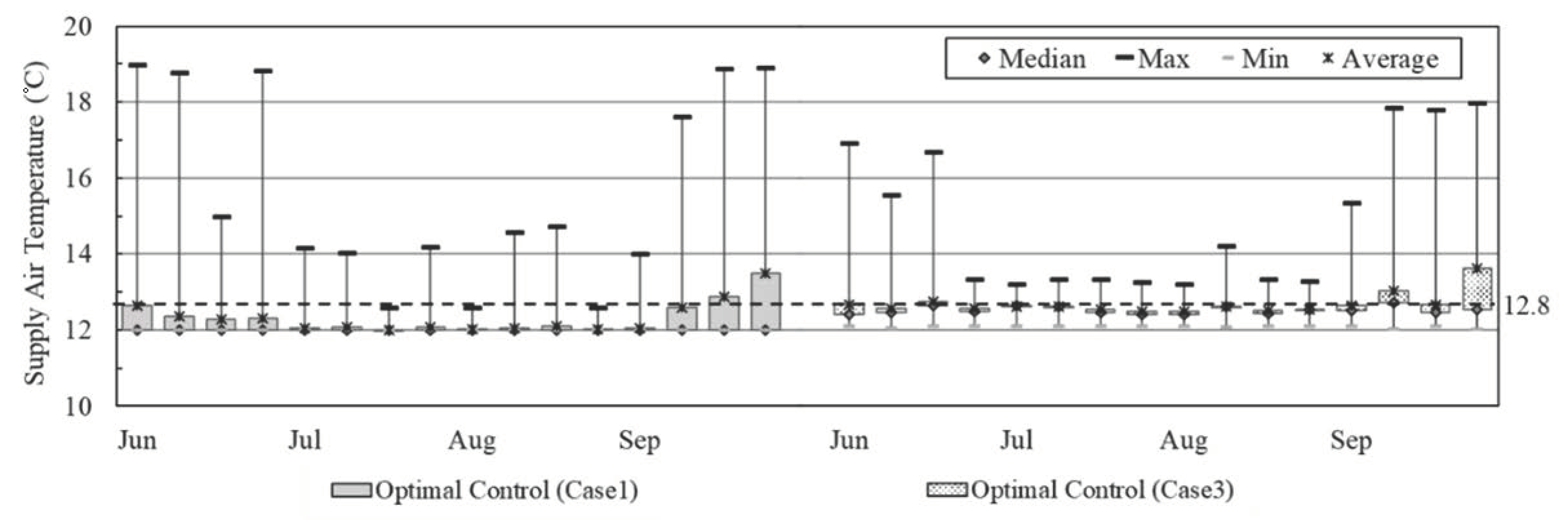
Figure 4 presents the changes in the supply air temperature from June to September. Among the proposed optimal control operation scenarios, case 2 does not include supply air temperature as a control variable, so the changes in supply air temperatures are shown only for case 1 and case 3. For both case 1 and case 3 in June and September, the distribution of the supply air temperature ranged from 12 °C, the lowest value, to 17–18 °C, which is not significantly different from the outside temperature. For case 1, the maximum value is 19 °C, which is the upper limit of the control range of the supply air temperature. In June and September, the building temperature can be controlled using a temperature that does not differ significantly from the outside air temperature. The results indicate that outside air cooling can be introduced without requiring the air conditioner to run when the cooling load is relatively low. The supply air temperature in July and August, when the cooling load increases, was operated at about 12 °C, the lowest value of the control range when controlled for case 1 and slightly lower than for normal operations when controlled for case 3 that operated at about 12.6 °C. If the supply air temperature is continuously set to a low supply air temperature, as in July and August, there is risk of condensation on the supply duct or outlet side, and reheating is required to maintain the indoor set temperature. In addition, cold drafts can also occur indoors, so these factors must be considered when applying operation methods.
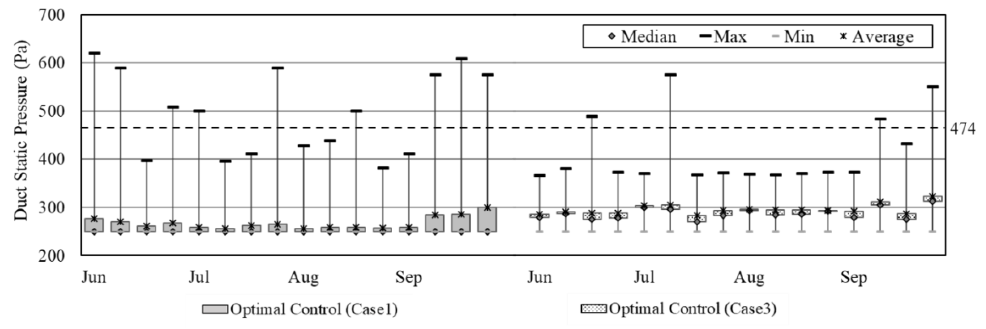
4.1.2. Duct Static Pressure
Figure 5 shows the changes in duct static pressure from June to September. Case 2 does not include duct static pressure as a control variable, so the changes in duct static pressure are shown only for case 1 and case 3. For both case 1 and case 3, the duct static pressure on the air supply side was kept below 474 Pa and kept constant during normal operations. Maintaining low duct static pressure in the system provides less air volume than the design air volume, which saves energy when using the blower. For case 1, the average duct static pressure per month was 268 Pa in June, 261 Pa in July, 258 Pa in August, and 283 Pa in September. However, the reduction in the amount of airflow due to maintaining the low duct static pressure may temporarily reduce the local indoor air quality in the zone due to the decrease in the airflow speed inside, even when meeting the required amount of outside air. Therefore, maintaining adequate indoor air quality is necessary.
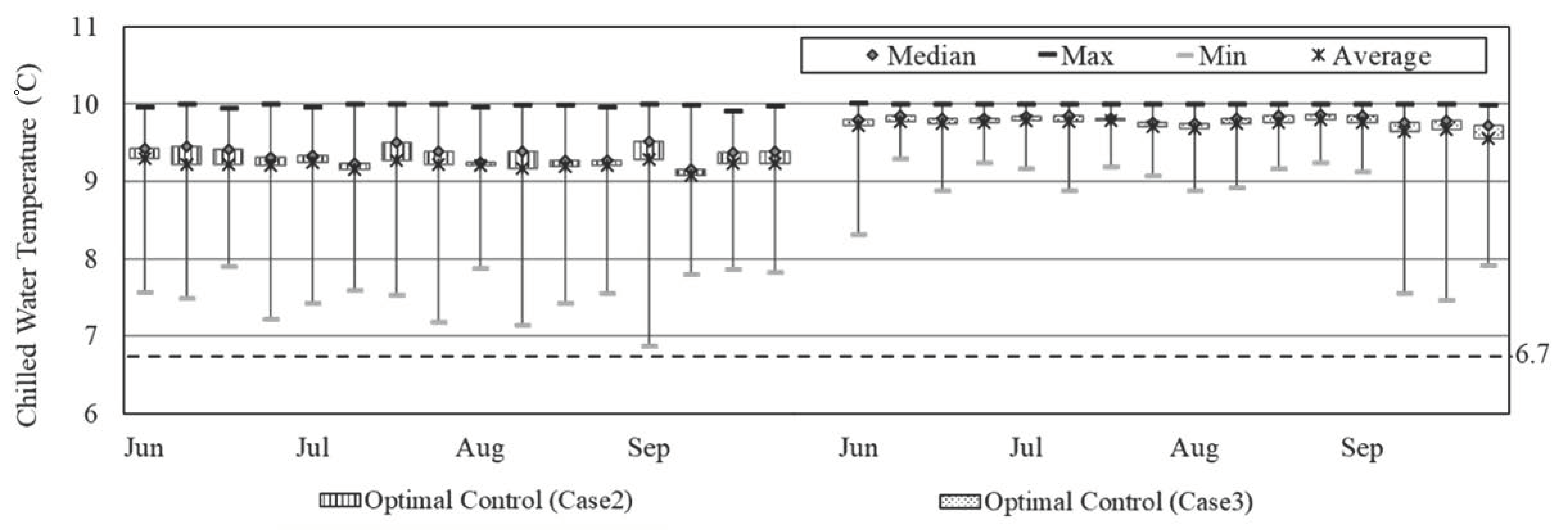
4.1.3. Chilled Water Temperature
Figure 6 shows the changes in the chilled water temperature from June to September. Both optimal control scenarios, case 2 and case 3, were operated between 9 and 10 °C higher than the chilled water temperature of 6.7 °C, which is set during normal operations according to the design value. In the optimal control operations, the cooling load of the building can be handled sufficiently, even with cold water that has a temperature higher than the design value of 6.7 °C. Therefore, energy consumption in the chiller can be reduced by reducing the power consumption of unnecessary compressors that typically are used to produce cold water at a low temperature in the chiller. This method also is expected to be able to detect and prevent over-cooling of the chiller. Moreover, it can be used to calculate the chilled water temperature that is suitable for the cooling load of the building or to calculate the chiller capacity (size).
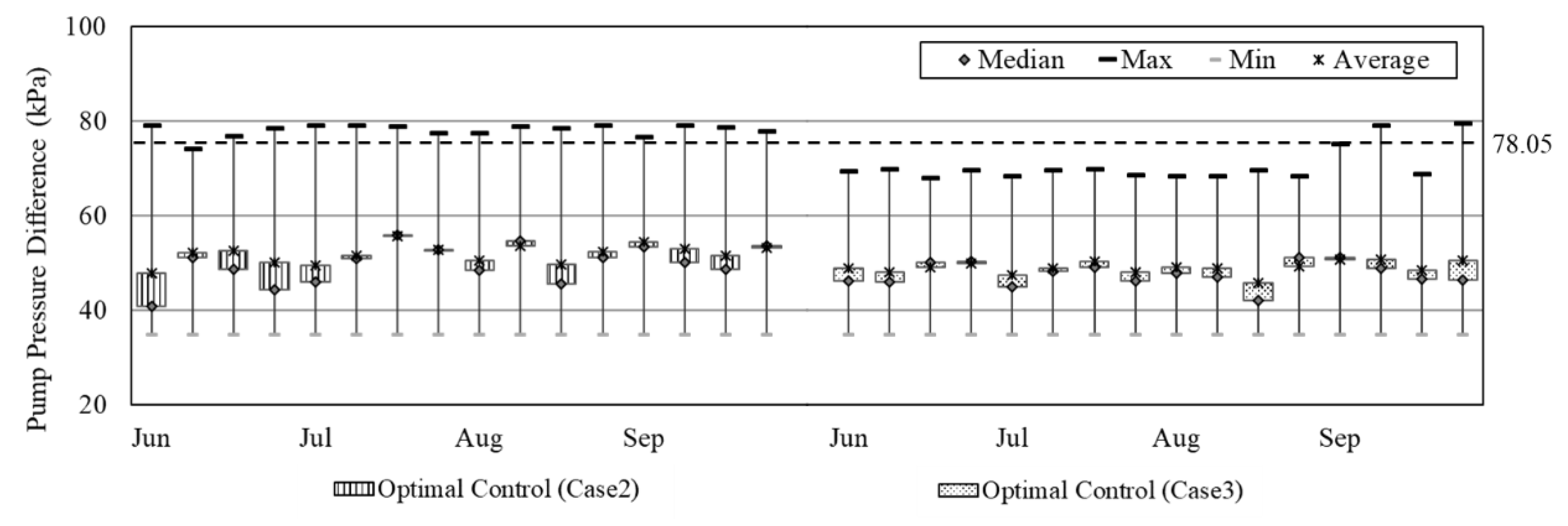
4.1.4. Pump Pressure Difference
Figure 7 shows the pump pressure differences associated with operation conditions from June to September. Both optimal control case 2 and case 3 operated while maintaining a lower value than the set value of 78.05 kPa, which is the difference in pump pressure during normal operations and the design value. The pump pressure differences for case 2 and case 3 averaged about 26.10 and 29.04 kPa, respectively. These scenarios can cool the reference building by maintaining a low chilled water pump pressure. When a low differential pressure is maintained in the chilled water loop, cooling is possible even with a small flow of cold water during operation of the HVAC system, which also results in the reduction of the head of the chilled water pump.
4.2. Analysis of Energy Consumption
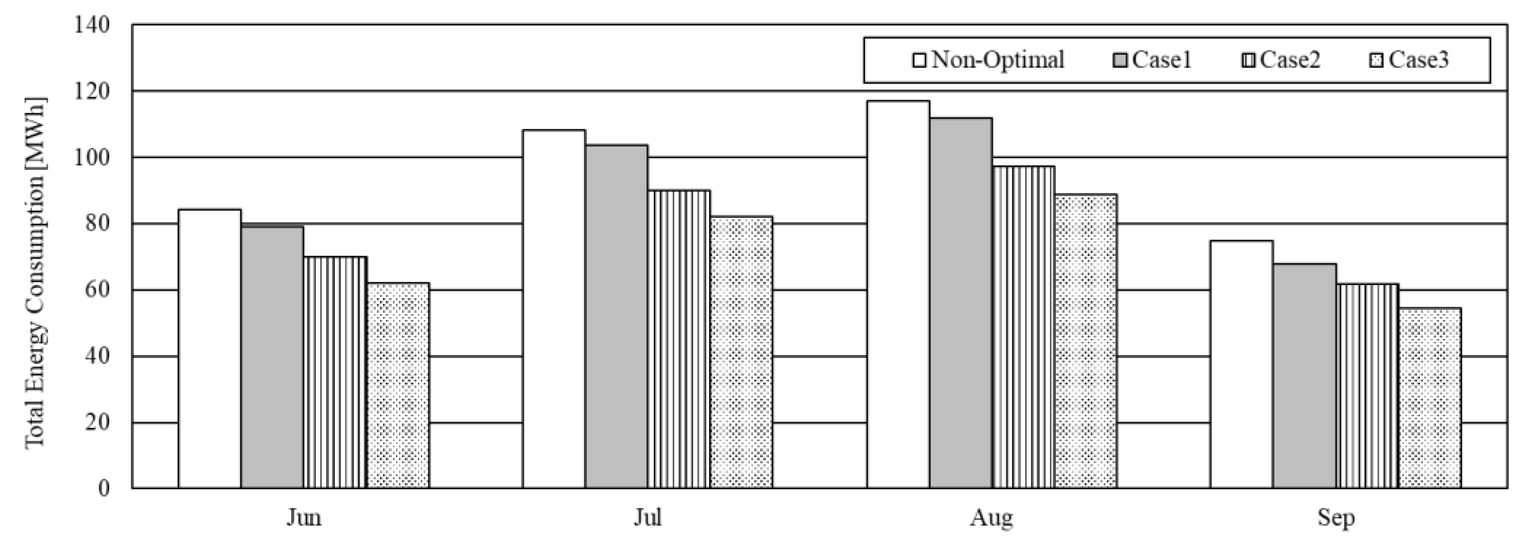
4.2.1. Monthly Energy Consumption Comparison
Figure 8 shows comparisons of the monthly energy consumption for normal operations as well as for each optimal control operation scenario from June to September, the period of analysis. Of all the optimal control operations in these months, case 3 saved the most energy by approximately 23.9% to 27.2%, case 2 saved approximately 16.6% to 17.53%, and case 1 saved approximately 4.2% to 9.6%. In other words, case 3, which uses all four control variables, had higher energy-saving percentages than case 1 and case 2; that is, as the number of control variables increased, the energy savings percentage also increased. The monthly energy saving ratios for case 1 and case 3 showed a difference of more than 2–3% in June and September compared to July and August when the cooling load was large, while case 2 showed similar savings rates within 1% of all months. The method of controlling the heat source side showed a constant variation in energy savings regardless of the change in cooling load.
4.2.2. Total Energy Consumption Comparison
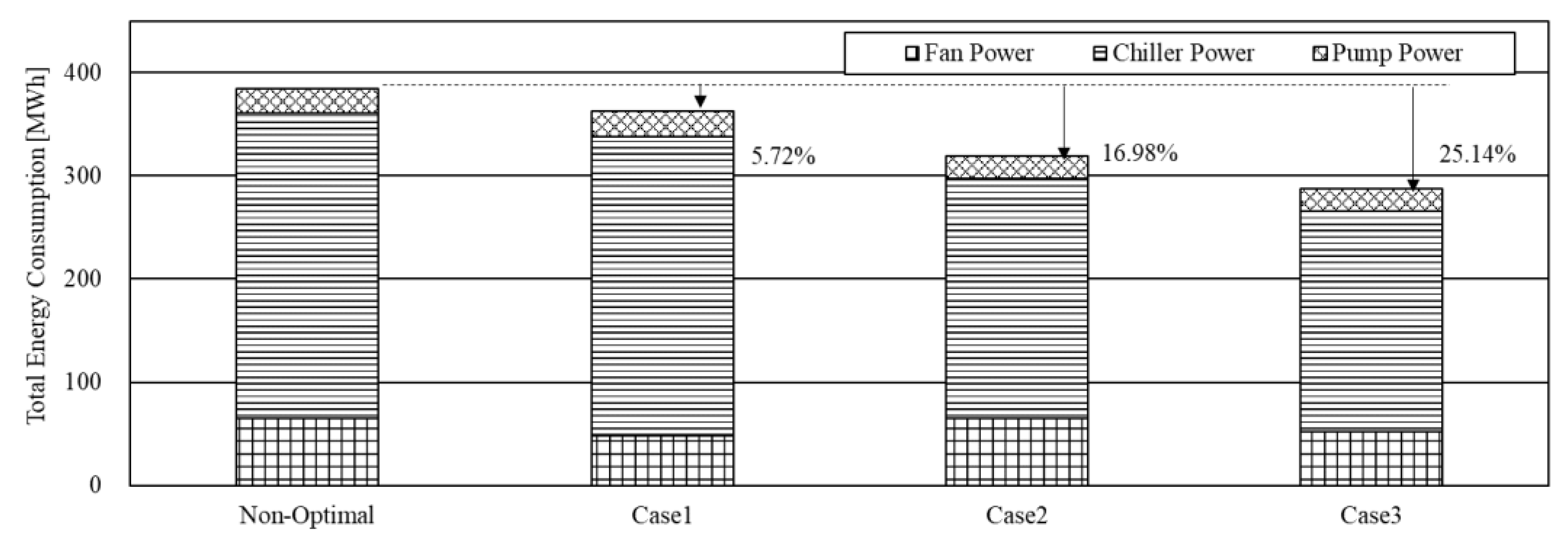
Figure 9 shows a comparison of the overall energy consumption under normal operations and under each optimal control operation scenario from June to September, the period of analysis. The total energy consumption comparison also confirms the energy savings effect due to an increase in the number of control variables. Although both case 1 and case 2 were controlled using only two control variables, the energy savings ratio differed by more than 10% due to the larger proportion of energy consumed by the chiller than the AHU (including the fan) in the target building.
4.2.3. Energy Consumption Comparison by Component
In this study, the energy consumption of the HVAC system was calculated as the sum of the energy consumption of the fan, chiller, and chilled water pump. Therefore, the changes in energy consumption by component also needed to be analyzed in order to understand how the characteristics of each optimal control operation affects the change in the energy consumption of each component for each case. The results are as follows.
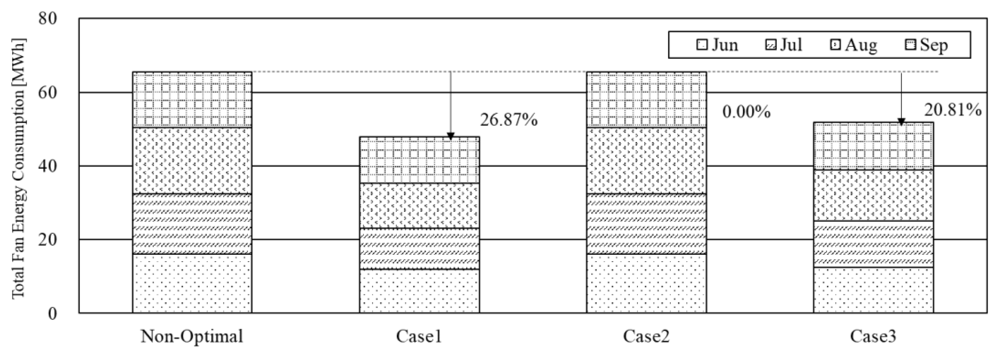
Figure 10 shows a comparison of the energy consumption of the fan according to normal operations and each optimal control operation scenario from June to September. Case 1 saved the most fan energy at 26.87%. Case 2 was unable to save blower energy because this case has no fan-related control variables. Although case 3 used all the control variables, the savings rate was approximately 6% lower than case 1, which is judged to be due to the output of the algorithm that considers a balance of the air-side variables and water-side variables in order to save energy of the chiller and cold water pump simultaneously while also using the chilled water temperature and pump pressure. Thus, case 1 is the most advantageous control method but only with regard to energy savings of the fan.
In buildings where AHU is designed to be larger than the chilled water plant, it is expected that greater energy savings can be achieved by selecting only the air-side duct static pressure and air temperature as the control variables.
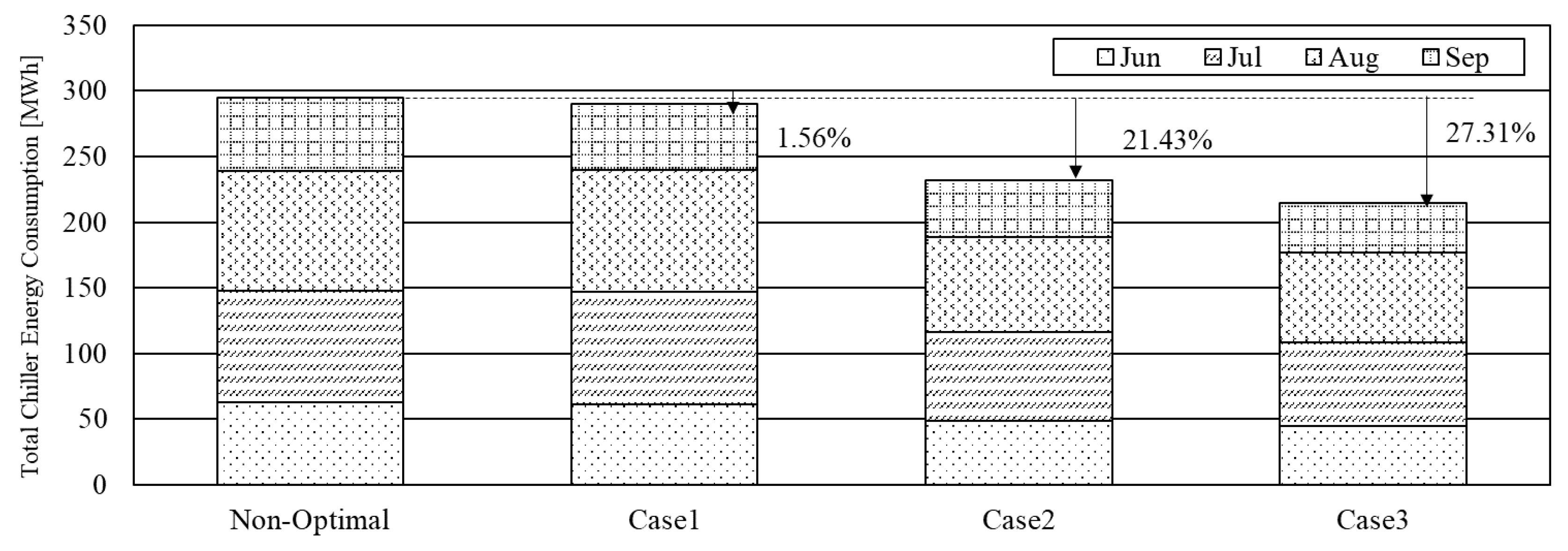
Figure 11 shows a comparison of the energy consumption of the chiller under normal operations and each optimal control operation scenario from June to September. Although in case 1, the control variables related to the chiller cannot be controlled directly, the energy consumption of the chiller decreased somewhat. The chiller is believed to have saved energy by being cooled directly via outdoor air intake when the outdoor air temperature was low and free cooling was possible. In case 2, the cooling load of the chiller could be handled sufficiently by supplying the chiller with cold water at a high temperature while the chiller operated between 9 and 10 °C, which is approximately 3 °C higher than the set point of 6.7 °C during normal operations. With more control variables, case 3 produced the more optimal chilled water temperature needed for cooling, compared to case 2, and saved the most chiller energy. The advantage here is that the chiller has many control variables for energy savings.
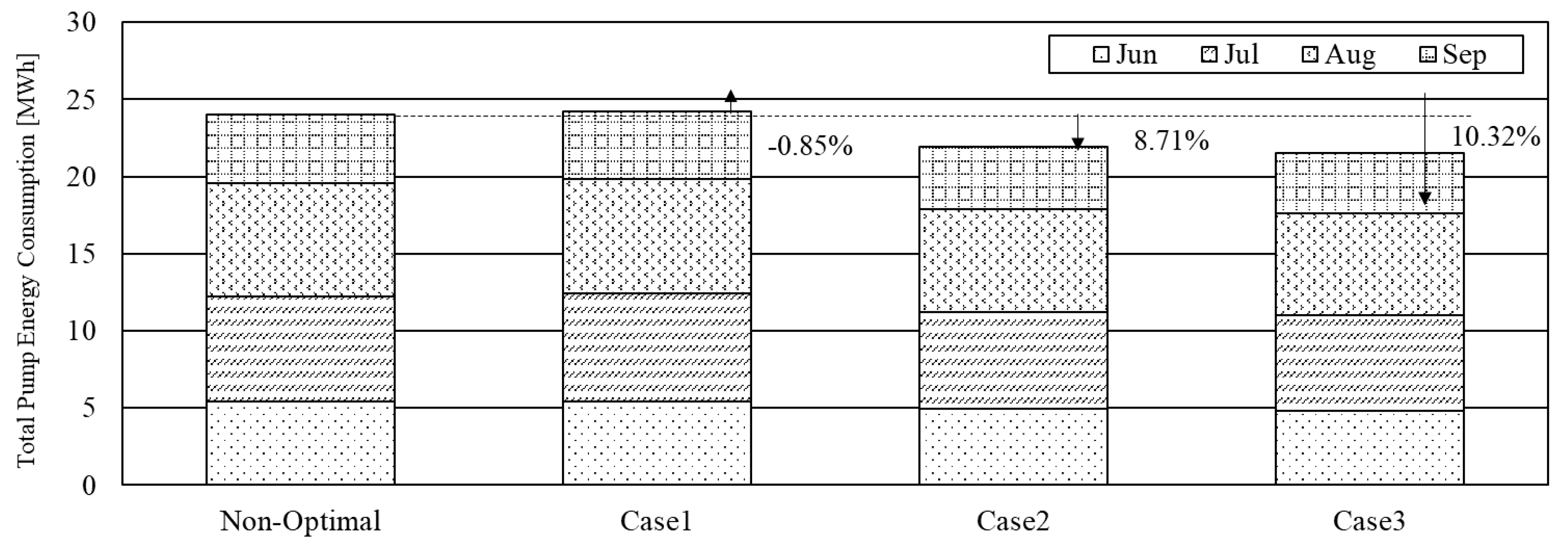
Figure 12 shows a comparison of the energy consumption of the cold-water pump under normal operations and under each optimal control operation scenario from June to September. In case 1, the energy consumption of the chilled water pump increased slightly due to the partial increase in the circulation of the cold water, as the cooling coil must be supplied with only the amount of chilled water that is needed to keep the supply air temperature low in the AHU. In case 2, the pump pressure difference was about 26 kPa lower than the set point of 78.05 kPa during normal operations, providing the load with a lower flow rate of chilled water and thus saving energy from the chilled water pump. Case 3 used all the control variables and operated the chilled water pump by supplying the more optimal chilled water flow rate compared to case 2, thereby saving the most energy.
To save the energy of the chilled water plant composed of the chiller and pump, control using many control variables could save more energy. The conditions of control variables in the AHU also have a significant effect on energy performance in optimizing the chilled water plant.
5. Conclusions
The optimal control variables used in an HVAC system were derived in this study using a GA. Three optimal control scenarios were established by varying the setting and number of optimal control variables. The three optimal control scenarios were compared and evaluated versus normal operating conditions by investigating changes in the appropriate optimal control variables and energy savings.
The change in the supply air temperature was 12.31 °C on average during operations with case 1 and 12.68 °C on average during operations with case 3, operating at a temperature approximately 0.5 to 0.3 °C lower than the set point of 12.8 °C during normal operations. The change in duct static pressure was 267 Pa on average for case 1 and 296 Pa for case 3, which is approximately 180 to 200 Pa lower than the set point of 474 Pa during normal operations. The optimal control variable derived using the GA is considered to have saved energy while maintaining the air supplied to each zone from the VAV system in a low-temperature to low-pressure state.
The change in chilled water temperature was 9.21 °C on average for case 2 and 9.73 °C on average for case 3, which was operated at a temperature 2.5–3.0 °C higher than the set point of 6.7 °C during normal operations. The change in pump differential pressure was 51.95 kPa on average for case 2 and 49.01 kPa on average for case 3 and was maintained at a differential pressure of about 26 to 29 kPa lower than the set point of 78.05 kPa during normal operations. The optimal control variable derived using the GA is considered to have saved energy while keeping the chilled water loop in a low-temperature low-pressure state.
The overall energy savings of the HVAC system during operations was 5.72% in case 1, 16.98% in case 2, and 25.14% in case 3. The control method of case 3 used all the control points and saved the most energy, up to approximately 25% for the target building using optimal control variables. The energy savings of the fan were best in case 1, and the energy savings of the chiller and chilled water pump were best in case 3.
The results of this study confirm that the energy savings percentage differs according to the change in the setting points and number of control variables. Additionally, the more multiple control points are optimized by increasing the number of control variables, the more effective is the energy savings. Therefore, the adjustment of multiple variables for optimal control is important when reviewing the effects of control, selection of variables, and control strategies. However, the size and operation conditions of each component in the HVAC system may vary as the location and weather condition, and the design and size of the building and the schedule for usage change, so the energy savings rate for each proposed optimal control operation scenario will vary.
In future research, there are also many other control variables in the HVAC system, so that additional research on optimal control operation in more complex control conditions should be carried out by adding a variety of control variables, and the optimal control proposed in this study should be verified in the on-site building.
Author Contributions
N.-C.S. contributed to the project idea development and wrote a draft version. J.-H.K. performed the data analysis. W.C. reviewed the final manuscript and contributed to the results, discussion, and conclusions. All authors have read and agreed to the published version of the manuscript.
Funding
This work is supported by the Korea Agency for Infrastructure Technology Advancement (KAIA) grant funded by the Ministry of Land, Infrastructure and Transport (20AUDPB099686-06).
Conflicts of Interest
The authors declare that there is no conflict of interests regarding the publication of this article.
References
- Tang, R.; Wang, S.; Shan, K. Optimal and near-optimal indoor temperature and humidity controls for direct load control and proactive building demand response towards smart grids. Autom. Constr. 2018, 96, 250–261. [Google Scholar] [CrossRef]
- Moradi, H.; Setayesh, H.; Alasty, A. PID-Fuzzy control of air handling units in the presence of uncertainty. Int. J. Therm. Sci. 2016, 109, 123–135. [Google Scholar] [CrossRef]
- Ginestet, S.; Marchio, D. Control tuning of a simplified VAV system: Methodology and impact on energy consumption and IAQ. Energy Build. 2010, 42, 1205–1214. [Google Scholar] [CrossRef]
- Afram, A.; Janabi-Sharifi, F. Theory and applications of HVAC control systems—A review of model predictive control (MPC). Build. Environ. 2014, 72, 343–355. [Google Scholar] [CrossRef]
- Serale, G.; Fiorentini, M.; Capozzoli, A.; Bernardini, D.; Bemporad, A. Model Predictive Control (MPC) for Enhancing Building and HVAC System Energy Efficiency: Problem Formulation, Applications and Opportunities. Energies 2018, 11, 631. [Google Scholar] [CrossRef]
- Afram, A.; Janabi-Sharifi, F.; Fung, A.S.; Raahemifar, K. Artificial neural network (ANN) based model predictive control (MPC) and optimization of HVAC systems: A state of the art review and case study of a residential HVAC system. Energy Build. 2017, 141, 96–113. [Google Scholar] [CrossRef]
- Peng, Y.; Rysanek, A.; Nagy, Z.; Schlüter, A. Using machine learning techniques for occupancy-prediction-based cooling control in office buildings. Appl. Energy 2018, 211, 1343–1358. [Google Scholar] [CrossRef]
- Drgoňa, J.; Picard, D.; Kvasnica, M.; Helsen, L. Approximate model predictive building control via machine learning. Appl. Energy 2018, 218, 199–216. [Google Scholar] [CrossRef]
- Nassif, N. Modeling and optimization of HVAC systems using artificial intelligence approaches. ASHRAE Trans. 2012, 118, 133–140. [Google Scholar]
- Papadopoulos, S.; Azar, E. Optimizing HVAC operation in commercial buildings: A genetic algorithm multi-objective optimization framework. In Proceedings of the 2016 Winter Simulation Conference (WSC), Washington, DC, USA, 11–14 December 2016; pp. 1725–1735. [Google Scholar]
- Satrio, P.; Mahlia, T.M.I.; Giannetti, N.; Saito, K. Optimization of HVAC system energy consumption in a building using artificial neural network and multi-objective genetic algorithm. Sustain. Energy Technol. Assess. 2019, 35, 48–57. [Google Scholar] [CrossRef]
- Seong, N.-C.; Kim, J.-H.; Choi, W. Optimal Control Strategy for Variable Air Volume Air-Conditioning Systems Using Genetic Algorithms. Sustainability 2019, 11, 5122. [Google Scholar] [CrossRef]
- Seong, N.C.; Kim, J.H.; Choi, W. Determination of optimal variables for chilled water loop in central air-conditioning system using genetic algorithms. J. Korean Inst. Archit. Sustain. Environ. Build. Syst. 2020, 14, 66–79. [Google Scholar] [CrossRef]
- Nassif, N.; AlRaees, N.; AlRifaie, F. Optimizing the Design of Chilled-Water Plants for Commercial Building Energy Systems. ASHRAE Trans. 2017, 123, 64–71. [Google Scholar]
- Asad, H.S.; Yuen, R.K.K.; Liu, J.; Wang, J. Adaptive modeling for reliability in optimal control of complex HVAC systems. Build. Simul. 2019, 12, 1095–1106. [Google Scholar] [CrossRef]
- Field, K.; Deru, M.; Studer, D. Using DOE commercial reference buildings for simulation studies. Proc. SimBuild 2010, 4, 85–93. [Google Scholar]
- ASHRAE. Energy Standard for Buildings Except Low-Rise Residential Buildings; ANSI/ASHRAE/IESNA Standard 90.1-2010; ASHRAE: Atlanta, GA, USA, 2010. [Google Scholar]
- Field, K.; Deru, M.; Studer, D. United States Department of Energy commercial reference building models of the national building stock. In Fourth National Conference of IBPSA; National Renewable Energy Laboratory: Golden, CO, USA, 2010; pp. 85–93. [Google Scholar]
- Deru, M.; Field, K.; Studer, D.; Benne, K.; Griffith, B.; Torcellini, B.; Liu, B.; Halverson, M.; Winiarski, D.; Rosenberg, M.; et al. U.S. Department of Energy Commercial Reference Building Models of the National Building Stock (NREL/TP-5500-46861); Technical Report; National Renewable Energy Laboratory: Golden, CO, USA, 2011.
- Kim, J.-H.; Seong, N.-C.; Choi, W. Modeling and Optimizing a Chiller System Using a Machine Learning Algorithm. Energies 2019, 12, 2860. [Google Scholar] [CrossRef]
- Huang, Q.; Rodriguez, K.; Whetstone, N.; Habel, S. Rapid Internet of Things (IoT) prototype for accurate people counting towards energy efficient buildings. J. Inf. Technol. Constr. 2019, 24, 1–13. [Google Scholar] [CrossRef]
- Arslan, M.; Cruz, C.; Ginhac, D. Understanding Occupant Behaviors in Dynamic Environments using OBiDE framework. Build. Environ. 2019, 166, 106412. [Google Scholar] [CrossRef]
- Tesiero, R.C., III. Intelligent Approaches for Modeling and Optimizing HVAC Systems. Ph.D. Thesis, North Carolina Agricultural and Technical State University, Greensboro, NC, USA, 2014. [Google Scholar]
- ASHRAE. ASHRAE Handbook-HVAC Systems and Equipment; ASHRAE: Atlanta, GA, USA, 2008. [Google Scholar]
| Publisher’s Note: MDPI stays neutral with regard to jurisdictional claims in published maps and institutional affiliations. |
© 2020 by the authors. Licensee MDPI, Basel, Switzerland. This article is an open access article distributed under the terms and conditions of the Creative Commons Attribution (CC BY) license (http://creativecommons.org/licenses/by/4.0/).


