Quantitative Evaluation of Corrosion Degrees of Steel Bars Based on Self-Magnetic Flux Leakage

Abstract

Corrosion is among the most critical factors leading to the failure of reinforced concrete (RC) structures. Less work has been devoted to nondestructive tests (NDT) to detect the corrosion degree of steel bars. The corrosion degree was investigated in this paper using an NDT method based on self-magnetic flux leakage (SMFL). First, a mathematic model based on magnetic dipole model was settled to simulate the SMFL of a V-shaped defect caused by corrosion. A custom 3-axis scanning device equipped with a magnetometer was used to scan the SMFL field of the 40 corroded steel bars. Experimental data obtained by scanning the 40 steel bars showed that the B_Z curve of SMFL was consistent with the theoretical model analysis. Inspired by the qualitative analysis of the results, an index “K” based on a large number of experimental data was established to characterize the corrosion degree of steel bars. The experimental index “K” was linearly related to the corrosion degree α of steel bars. This paper provides a feasible approach for the corrosion degree NDT, which is not affected by the magnetization history and the initial magnetization state of steel bars.

1. Introduction

The reinforced concrete (RC) structure is the most common structure in civil engineering, because steel bar and concrete can work together to fully exert their mechanical properties, thus forming good force-bearing members [1]. However, corrosion is among the most important factors leading to the failure of RC structures. Corrosion is a critical determinant of stress concentration as a consequence of the reduction of the cross-sectional region of a steel bar [2,3]. Moreover, the volume expansion of the corrosion product will crack the weak part of the concrete, further weakening the bearing capacity of the RC structures [4].

For the reasons above, steel corrosion is a continuing concern within civil engineering and the issue of nondestructive testing (NDT) has received considerable critical attention. One of the main obstacles in detecting corrosion by a typical NDT method, visual testing (VT), is that the steel bars are usually inside the RC structures. Except for VT, studies over the past three decades have provided many practical NDT methods on metals, such as ultrasonic diffraction time difference (TOFD) [5], acoustic emission (AE) [6,7,8], ultrasonic testing (UT) [9,10,11], radiographic testing (RT) [12], and electromagnetic detection. Among these methods, electromagnetic detection has been popular in recent years. It includes eddy current inspection [13], magnetic Barkhausen emission (MBE), magneto-acoustic emission (MAE) [14], metal magnetic memory (MMM) [15], magnetic flux leakage (MFL), and self-magnetic flux leakage (SMFL).

More and more researchers are using electromagnetic NDT to detect metal defects. Park [16] studied magnetic Barkhausen emission (MBE) and magneto-acoustic emission (MAE) signals to evaluate the effects of radiation in RPV steel. Chen [17] studied the stress-magnetic effect of ferromagnetic materials based on three-dimensional magnetic flux leakage (MFL). Dong [18] explored the metal magnetic memory (MMM) test for early damage assessment of ferromagnetic materials. Sawade [19] applied MFL as an NDT method for prestressed concrete structures. Pang [20] used MMM for internal force detection of RC structures. Recently, researchers have focused the effects of corrosion on self-magnetic flux leakage (SMFL) signals. The principle of SMFL is that the magnetic field generated by the ferromagnetic material under the excitation of the earth’s magnetic field will have some abnormal magnetic field changes in the defect region of the ferromagnetic materials. Several attempts have been made to explore the usage of SMFL in corrosion detection. Zhang [21] used the SMFL to detect the corrosion of steel bars and proposed that the steel corrosion region will improve the magnetic resistivity for SMFL, which results in abnormal magnetic field distribution. Xia [22] used SMFL to quantitatively analyze the corroded steel strands and proposed three growth models (logistic growth model, exponential growth model, and linear growth model) to simulate the variation of the coefficient A in the magnetic dipole model. A possible correlation between the bearing capacity of the strand and the SMFL signal was also introduced in his study. Qiu [23] conducted a series of four-point experiments that focused on the bending strength of RC beams to estimate a possible correlation between the SMFL signals and the bearing capacity of RC beams. His works also confirmed that SMFL is hardly affected by stirrups. Qu [24] combined SMFL with numerical analysis method of the magnetic dipole model to test the corrosion width of the steel strand.

Inspired by the several researches introduced above, it can be speculated that the SMFL signals of the steel bar should be related to its degree of corrosion. In practical scenarios, construction workers usually pour concrete when the steel bars are slightly corroded in order to improve the bonding performance between the steel bars and the concrete [1]. Therefore, not all steel bar corrosion conditions are unfavorable in civil engineering applications. However, the testing method associated with corrosion degree had been a largely under explored domain. To this end, a model based on SMFL is established to test the correlation between SMFL signals and the corrosion degree of steel bars.

Compared with the MFL detection, SMFL eliminates the complicated manual excitation magnetization step. In addition, it has the characteristics of fast diagnosis, simple operation, low price, and light sensor [21,22,23]. The SMFL approach is an advanced method. Especially for the case where the surface of the material is defective, SMFL is highly reliable and accurate [21]. However, because it is susceptible to magnetization history and initial magnetization state, quantitative analysis of SMFL signals remains a major challenge [22].

This study aims to contribute to an NDT method to detect the corrosion degree in RC structures. The remaining part of the paper is as follows: A detailed material preparation and mathematical model will be presented in Section 2. Section 3 analyzes the result of the experiment, and the conclusions will be provided. Finally, all the results will be summarized in Section 4.

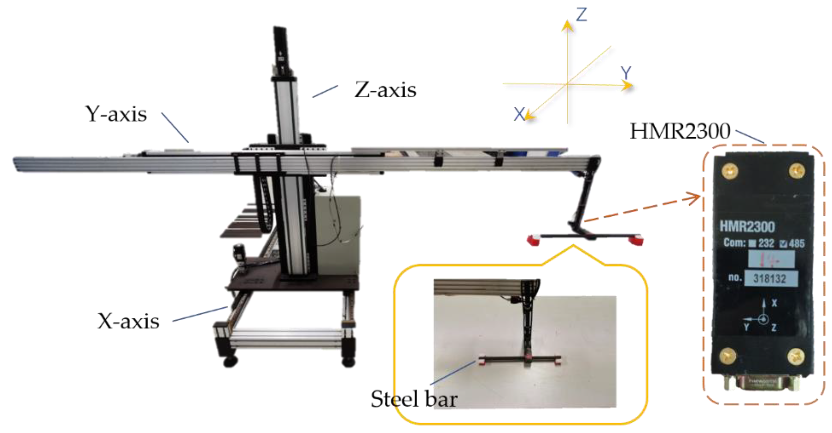
2. Materials and Methods

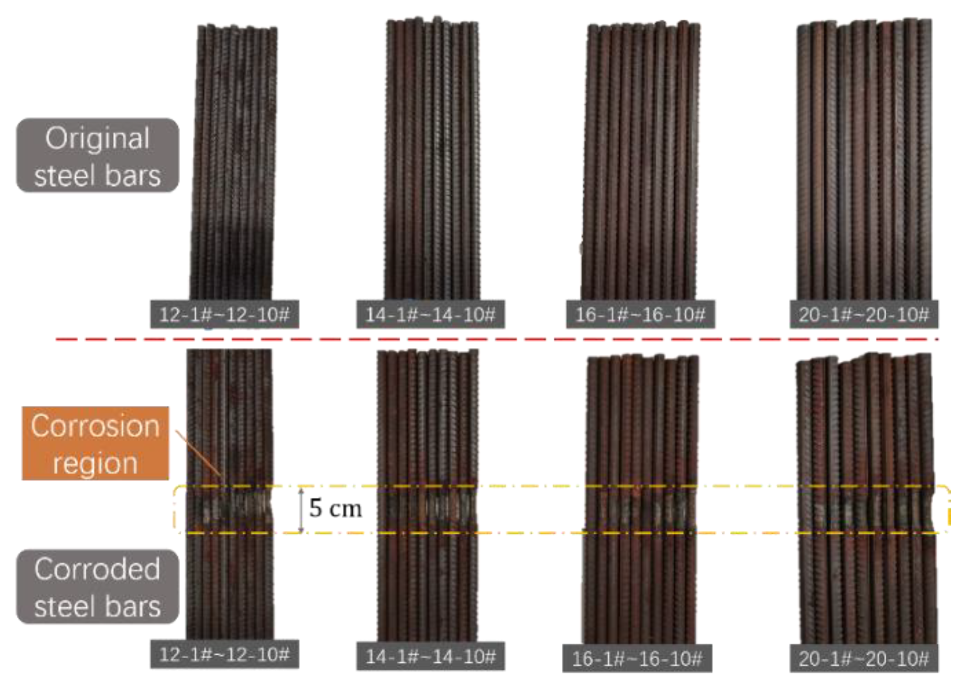
2.1. Material Preparation

Forty HRB400 ribbed steel bars with lengths of 50 ± 1 cm were selected as experimental samples to evaluate the performance of the model based on SMFL. The material parameters are shown in

Table 1. Material parameters of steel bars.

Type of Steel	Diameter/mm	Density g/cm2	Component, wt.%
			C	Mn	Si	P	S
HRB400	12	7.9	0.22	1.4	0.5	0.02	0.01
	14
	16
	20

. The steel bars were cut to the required length (50 cm) using a circular saw, and there were 10 steel bars in each group of different diameters. After the steel bars were cut, the magnetic byproduct Fe₃O₄, generated during the cutting process, was carefully removed from the steel bars. Demagnetization was conducted before experiment to remove magnetic fields caused by high temperature [25]. After the processing of steel bars, they were numbered 12-1#–12-10#, 14-1#–14-10#, 16-1#—16-10#, and 20-1#—20-10#, respectively. To compare the SMFL signals with the steel bars after corrosion, these 40 steel bars were scanned by a HMR2300 magnetometer (Honeywell, Charlotte, NC, USA) before being corroded.

The corrosion of steel bars under natural conditions is a long process, and the location and extent of corrosion is difficult to control. It is an electrochemical process, and its occurrence has three prerequisites [26]:

(1)

There is a potential difference on the surface of the steel bar to form a corroded battery;

(2)

The passivation film on the surface of the steel bar is destroyed and is in an activated state;

(3)

Water and oxygen required for electrochemical reaction and ion diffusion are on the surface of the steel bar.

Therefore, in order to obtain corroded steel bars that met the requirements more quickly in the laboratory, an electrochemical accelerated corrosion method was employed. The shape of the steel corrosion region, which was obtained according to the existing accelerated corrosion method, is a V-shaped dent as shown in Figure 1.

According to the first law of Faraday’s electrolysis, the quality of corroded steel bars under the condition of time T and current I was calculated as:

$$m_{s0}=C\times {\displaystyle {\int }_0^{T}idi}$$

(1)

where C is a constant which can be determined by the material itself. The experimental environment allowed the law to be rewritten as:

$$m_{s0}=\frac{25}{24}\times I\times T$$

(2)

A model of steel corrosion was built to estimate the time and current required to reach the specified degree of corrosion, as shown in the

Table 2. The corrosion schedule of all samples.

Number	T/h	I/A	S/%	dm/mm	Number	T/h	I/A	S/%	dm/mm
12-1#	0	1.09	0	12.00	16-1#	0	1.29	0	16.00
12-2#	2	1.09	10.0	11.38	16-2#	3	1.29	10.0	15.17
12-3#	4	1.09	20.0	10.73	16-3#	6	1.29	20.0	14.31
12-4#	6	1.09	29.7	10.06	16-4#	9	1.29	29.7	13.42
12-5#	8	1.09	39.1	9.36	16-5#	12	1.29	39.1	12.49
12-6#	10	1.09	48.3	8.63	16-6#	15	1.29	48.3	11.51
12-7#	12	1.09	57.1	7.86	16-7#	18	1.29	57.1	10.48
12-8#	14	1.09	65.6	7.04	16-8#	21	1.29	65.6	9.39
12-9#	16	1.09	73.6	6.17	16-9#	24	1.29	73.6	8.23
12-10#	18	1.09	81.0	5.23	16-10#	27	1.29	81.0	6.97
14-1#	0	1.49	0	14.00	20-1#	0	1.52	0	20.00
14-2#	2	1.49	10.0	13.27	20-2#	4	1.52	10.0	18.96
14-3#	4	1.49	20.0	12.52	20-3#	8	1.52	20.0	17.89
14-4#	6	1.49	29.7	11.74	20-4#	12	1.52	29.7	16.77
14-5#	8	1.49	39.1	10.92	20-5#	16	1.52	39.1	15.61
14-6#	10	1.49	48.3	10.07	20-6#	20	1.52	48.3	14.39
14-7#	12	1.49	57.1	9.17	20-7#	24	1.52	57.1	13.10
14-8#	14	1.49	65.6	8.22	20-8#	28	1.52	65.6	11.74
14-9#	16	1.49	73.6	7.20	20-9#	32	1.52	73.6	10.23
14-10#	18	1.49	81.0	6.10	20-10#	36	1.52	81.0	8.72

. The steel bars were numbered in the item “Number”, while time and current required for each steel bar are listed in “T/h” and “I/A”, respectively. To obtain several degrees of corrosion, theoretical maximum cross-sectional loss rates of the samples are listed in “S%”. Nominal diameter of the corresponding steel bar is recorded in “d_m”.

The prepared steel bars were placed above containers, and towels were carefully wrapped in 5-cm lengths on the middle of the steel bars. In order to avoid the towels from spreading or falling off during the experiment, the towels were bundled with insulated wires. The positive poles of the current source were thin copper wires wound around one end of the steel bars. Correspondingly, the negative ones were carbon rods, which were placed in the containers and were in contact with towels soaked with 5% sodium chloride solution to form closed circuits. Due to the heat generated during the electrochemical acceleration of the corrosion, moisture in the towels evaporated quickly. To ensure that the towels were infiltrated by the 5% sodium chloride solution during the whole corrosion process, the 5% sodium chloride solution was continuously dripped into the towel by applying the siphon principle. The entire corrosion device layout is shown in the Figure 2.

A custom three-axis magnetic signals scanning device was applied to the experiment. The device was generally composed of supports, tracks, a control box, a magnetometer HMR2300, and a computer. The layout of the entire scanning device is shown in Figure 3.

Set by a computer program, the scanning path, scanning speed, and signals acquisition frequency of the three-axis scanning device can be determined. The scanning range is 200–700 mm for the Y axis, 200 mm for the X axis, and 5–350 mm for the Z axis, while the stepping speeds of each axis are all 500 mm/min. Data for this study were collected using a magnetometer HMR2300 manufactured by Honeywell, USA, which can be connected to a computer and output SMFL components B_X, B_Y, and B_Z. An acquisition period of the SMFL signal by the HMR2300 is 500 ms. To investigate the influence of HMR2300 lift-off height (LFH) on SMFL, five scanning paths were set as 5, 10, 40, 80, and 350 mm high from the samples, respectively, as shown in Figure 4.

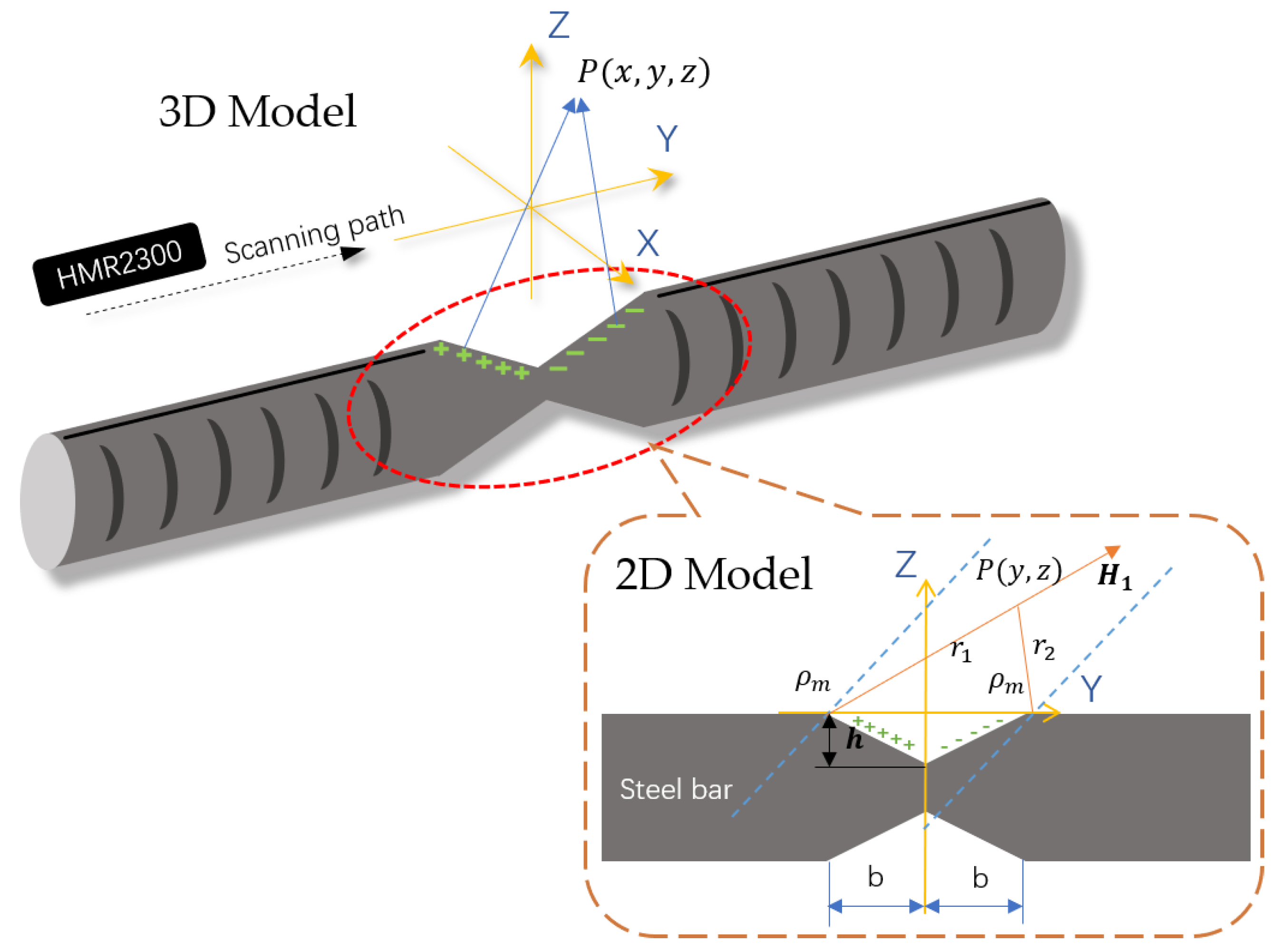
2.2. Mathematical Model

According to the existing magnetic dipole model, the magnetic field of the material when the ferromagnetic material is corroded can be simulated. From a variety of studies [27,28,29,30], it has been well-established that the exterior magnetic field of ferromagnetic material would be considered to originate from the magnetic charge ρ, which can be described as the following equation:

$$\rho =-\nabla \cdot \mathit{M}$$

(3)

where the magnetization vector M is adjacent to the edge of the defect. The theory of magnetic dipoles suggests that the leakage magnetic field at the defect of ferromagnetic material is generated by a dipole of opposite polarity. This phenomenon can be visually described as the magnetic line of ferromagnetic material leaking out at the defect, thus forming a tiny magnetic pole.

Many recent studies [22,23] have shown that the component of SMFL signals in the Bx direction is uninterpretable. For the purpose of simplifying the problem in a reasonable way, the 3D model should be converted into a 2D model as shown in Figure 5. The two broken lines shown in the 2D model are magnetic charge lines whose line magnetic charge densities are both ρ_m and the distance between them is 2b. The magnetic field generated by the broken lines at any point P (y, z) on the YOZ plane can be expressed as:

$${\mathit{H}}_1=\frac{2{\rho }_m}{r_1^2}{\mathit{r}}_1$$

(4)

$${\mathit{H}}_2=\frac{2{\rho }_m}{r_2^2}{\mathit{r}}_2$$

(5)

where r₁ and r₂ are the vectors from point P to the magnetic charge lines. The components of the vector element dH_p of SMFL along the y, z direction can be written as:

$$d{\mathit{H}}_{\mathit{p}}={\displaystyle \sum _{i=1}^{2}d{\mathit{H}}_{\mathit{p}\mathit{i}}}={\displaystyle \sum _{i=1}^2\frac{\pm {\rho }_{m}d{s}_i}{2\mathsf{\pi }{\mu }_0{r}_i^2}{\mathit{r}}_i^2}$$

(6)

$$\{\begin{array}{l}d{\mathit{H}}_1=\left[\begin{array}{l}d{H}_{1\mathrm{y}}\\ d{H}_{1\mathrm{z}}\end{array}\right]=\frac{{\rho }_m\sqrt{1+{\mathrm{b}}^2/{\mathrm{h}}^2}d\eta }{2\mathsf{\pi }{\mu }_0\left[{\left(y+\mathrm{b}+\eta \times \mathrm{b}/\mathrm{h}\right)}^2+{\left(z-\eta \right)}^2\right]}\left(\begin{array}{c}y+\mathrm{b}+\eta \times \mathrm{b}/\mathrm{h}\\ z-\eta \end{array}\right)\\ d{\mathit{H}}_2=\left[\begin{array}{l}d{H}_{2\mathrm{y}}\\ d{H}_{2\mathrm{z}}\end{array}\right]=\frac{{\rho }_m\sqrt{1+{\mathrm{b}}^2/{\mathrm{h}}^2}d\eta }{2\mathsf{\pi }{\mu }_0\left[{\left(y-\mathrm{b}-\eta \times \mathrm{b}/\mathrm{h}\right)}^2+{\left(z-\eta \right)}^2\right]}\left(\begin{array}{c}y-\mathrm{b}-\eta \times \mathrm{b}/\mathrm{h}\\ z-\eta \end{array}\right)\end{array}$$

(7)

where the constant μ₀ = 4π × 10⁻⁷ H/m. Note that H_z is the only component to be considered in this paper. The H_z can be calculated as:

$$H_Z={\displaystyle {\int }_{-h}^{0}d{H}_{1Z}}+{\displaystyle {\int }_{-h}^{0}d{H}_{2Z}}$$

(8)

The equation shown above leads to an analytical solution of the SMFL around the surface of a V-shaped defect. Thus, the magnetic field strength component H_z of a random point P (y, z) on the YOZ plane becomes:

$$H_Z=\frac{{\rho }_m\sqrt{1+{\mathrm{b}}^2/{\mathrm{h}}^2}}{2\mathsf{\pi }{\mu }_0}\left[\frac{1}{2\mathrm{A}}ln\left|\frac{{\mathrm{A}}_2\mathrm{h}+B_2\mathrm{h}+C_2}{{\mathrm{A}}_1\mathrm{h}+B_1\mathrm{h}+C_1}\right|+\left(Z-\frac{B_1}{2{\mathrm{A}}_1}\right)\times \frac{1}{\sqrt{{\Delta }_1}}\times \left(acrtan\frac{B_1}{\sqrt{{\Delta }_1}}-acrtan\frac{B_1-2{\mathrm{A}}_1\mathrm{h}}{\sqrt{{\Delta }_1}}\right)-\left(Z-\frac{B_2}{2{\mathrm{A}}_2}\right)\times \frac{1}{\sqrt{{\Delta }_2}}\times \left(acrtan\frac{B_2}{\sqrt{{\Delta }_2}}-acrtan\frac{B_2-2{\mathrm{A}}_2\mathrm{h}}{\sqrt{{\Delta }_2}}\right)\right]$$

(9)

where A, A₁, A₂, B₁, B₂, C₁, C₂, ∆₁, and ∆₂ are related to y, z, b, and h.

$$\{\begin{array}{l}{\mathrm{A}}_1={\mathrm{A}}_2=\mathrm{A}=\frac{{\mathrm{b}}^2}{{\mathrm{h}}^2}+1\\ B_1=2[\frac{(y+\mathrm{b})\mathrm{b}}{\mathrm{h}}-z]\\ B_2=2[\frac{(\mathrm{b}-y)\mathrm{b}}{\mathrm{h}}-z]\\ C_1=y^2+2\mathrm{b}y+{\mathrm{b}}^2+z^2\\ C_2=y^2-2\mathrm{b}y+{\mathrm{b}}^2+z^2\\ {\Delta }_1=B_1^2-4\mathrm{A}{C}_1\\ {\Delta }_2=B_2^2-4\mathrm{A}{C}_2\end{array}$$

(10)

The H_Z curves of the mathematical model are shown in Figure 6. According to related research [21], H_Z curves of other defect shapes are similar in shape.

3. Results & Discussion

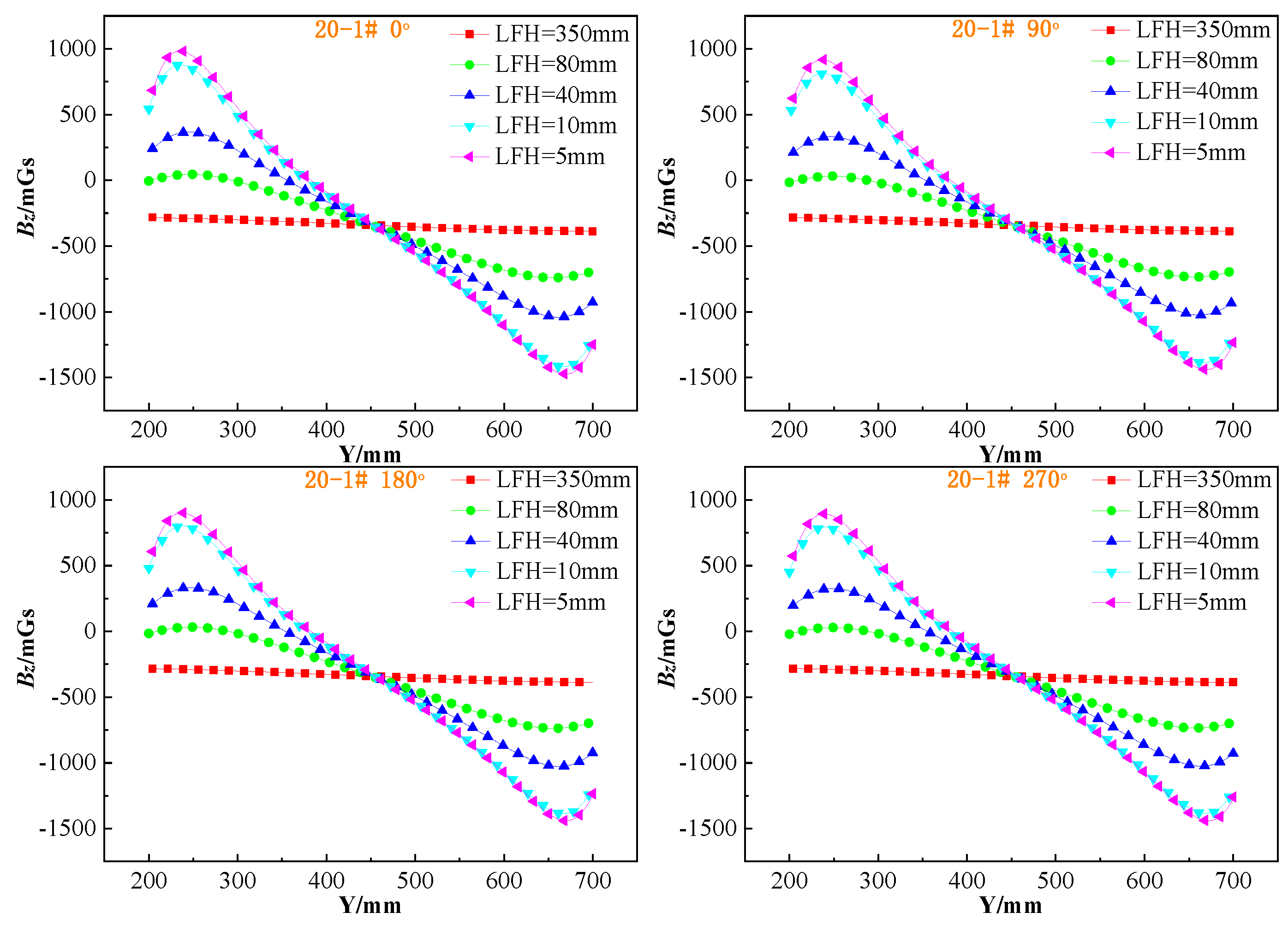
3.1. Experimental Result of Corrosion and SMFL Signals

A more detailed account of experimental results is given in the following section. For the purpose of analysis, the corrosion of each steel bar was carefully checked after the corrosion process. The corrosion regions were in the middle of the steel bars and their widths were about 5 cm. Comparison results of experimental samples before and after corrosion are displayed in Figure 7. As can be seen in the Figure 7, the degree of corrosion increases as the serial number of steel bars increases. Compared to theoretical results, the minimum diameters of each corroded steel bar were measured by using a caliper.

Table 3. The contrast of theoretical results and experimental results.

Number	D0/mm	Dc/mm	Number	D0/mm	Dc/mm
12-1#	11.39	11.39	16-1#	15.28	15.28
12-2#	10.99	10.69	16-2#	15.27	14.75
12-3#	11.37	9.93	16-3#	15.37	14.27
12-4#	11.21	9.30	16-4#	15.37	13.56
12-5#	11.42	9.51	16-5#	15.41	12.93
12-6#	11.42	8.62	16-6#	15.33	12.82
12-7#	11.05	8.29	16-7#	15.25	12.67
12-8#	11.47	8.24	16-8#	15.35	12.86
12-9#	11.40	6.94	16-9#	15.25	9.86
12-10#	11.38	5.68	16-10#	15.32	10.82
14-1#	13.14	13.14	20-1#	19.17	19.17
14-2#	13.05	12.49	20-2#	19.03	18.55
14-3#	13.23	12.16	20-3#	19.17	17.98
14-4#	13.07	11.64	20-4#	19.02	17.04
14-5#	13.15	10.95	20-5#	19.07	16.97
14-6#	13.06	10.11	20-6#	19.04	16.53
14-7#	12.84	9.13	20-7#	19.16	16.05
14-8#	13.19	9.46	20-8#	19.02	15.17
14-9#	13.05	9.36	20-9#	19.17	14.45
14-10#	13.12	9.17	20-10#	19.05	13.84

compares the experimental data on the steel bars before and after corrosion, where “D₀” and “D_C” are the measured diameter of original steel bar and the measured diameter of corroded steel bar, respectively.

Four angles of each steel bar were scanned to acquire data after careful inspection. To intuitively compare the differences of B_Z curves between original steel bars and those of corroded ones, figures of the signals in B_Z direction of these SMFL signals were drawn by using Origin software. With a qualitative analysis of these figures, it can be preliminarily concluded that the B_Z component of the SMFL signal is related to the corrosion degree of the steel bars. Through random sampling of several samples (12-8#, 14-4#, 16-5#, 20-5#) and comparing the B_Z curves of these different diameters of steel bars, it can be found that these curves are similar in shape as shown in Figure 8. The results of multiple scans of a steel bar in the same state were consistent, as shown in Figure 9, indicating that the SMFL was stable. In addition, it is not difficult to find from the figures that the SMFL curves of the same steel bar at different angles (0, 90, 180, 270) remain stable. From this, a conclusion can be reached that the degree of corrosion is uniform in the hoop direction of the steel bars. This also confirms that it is feasible to convert the mathematical model from three-dimensional to two-dimensional. The above-mentioned properties of the SMFL signals had significant benefits for an NDT method.

The results, as shown in Figure 10, indicated that the curves of B_Z component had a maximum or minimum value near the ends of the steel bars. This was because the residual stress formed during the cutting process had an irreversible effect on the SMFL of the steel bars. It should be noted that except for the curve fluctuation caused by the residual stress at both ends of the uncorroded steel bars, the B_Z curve was uniformly changed within the range of 5 to 45 cm in the middle of the steel bars without an extreme value. In the case of the corroded steel bars, the most obvious change of the B_Z component of the SMFL signal occurred in the middle of the steel bar, where B_Z curve exhibited an abnormal fluctuation and the maximum and minimum values appeared again. Moreover, the signal of the steel SMFL had a strong correlation with the LFH. The results showed that the lower the LFH, the more obvious the changes in the curves. By observing a plurality of sets of pictures, it was found that the positions of the peaks and troughs appearing in the middle of the B_Z curve of the corroded steel bars are near the endpoints of the corrosion region. It is therefore likely that such correlation exists between B_Z component of SMFL and corrosion degrees.

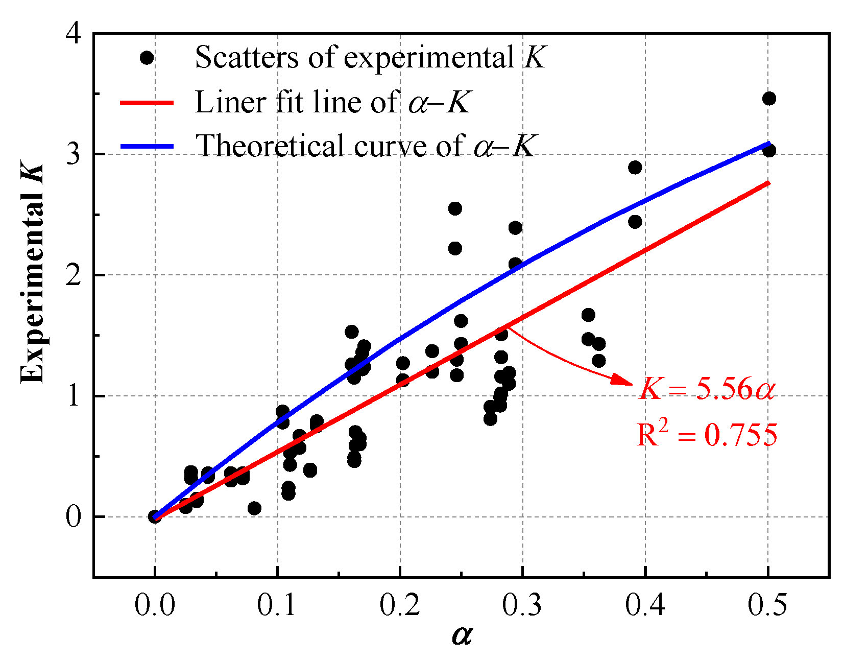
3.2. Quantitative Evaluation of SMFL for Steel Corrosion

As mentioned in the experimental results, it can be visually seen that the corrosion of the steel bars would cause a significant change in the B_Z component within the corroded regions, while the corrosion-free regions had no significant change. This rule was in good agreement with the theoretical analysis. In addition, the more severe corrosion of steel bars, the greater the variation of the B_Z component of the SMFL field in the corrosion region. Still, this is not sufficiently rigorous and intuitive to determine the degree of corrosion of the steel. In order to quantitatively explain the correlation between the degree of corrosion of the steel bars and the B_Z component of the SMFL field, the gradient parameter “G” is introduced, which is defined as follows:

$$G=max\left\{d_1,d_2,\dots ,d_{\mathrm{n}}\right\}$$

(11)

where d₁, d₂ ... d_n are the first derivative at each point of the B_Z curve within the corrosion region (assuming there are n points in the corrosion region).

Conforming to the definition of the gradient parameter “G”, the data was processed by Origin software and the experimental gradients G of the B_Z component curves were obtained. It should be noted that the B_Z component curves of the four angles (0, 90, 180, and 270) were collected during the experiment and the previous analysis revealed that there was no significant difference in the B_Z component curves at different angles. Therefore, the experimental gradients G of the four angle B_Z component curves were calculated separately and their mean values were taken. Subsequently, the experimental corrosion degree ratio α, which reflects the relative corrosion degree of steel bars, can be calculated as:

$$\alpha =\frac{D_0-D_c}{D_0}$$

(12)

The α of 40 samples can be calculated according to Table 3, as shown in

Table 4. The experimental corrosion degree ratio α of all samples.

Number	α	Number	α	Number	α	Number	α
12-1#	0.00	14-1#	0.00	16-1#	0.00	20-1#	0.00
12-2#	0.03	14-2#	0.04	16-2#	0.03	20-2#	0.03
12-3#	0.13	14-3#	0.08	16-3#	0.07	20-3#	0.06
12-4#	0.17	14-4#	0.11	16-4#	0.12	20-4#	0.10
12-5#	0.17	14-5#	0.17	16-5#	0.16	20-5#	0.11
12-6#	0.24	14-6#	0.23	16-6#	0.16	20-6#	0.13
12-7#	0.25	14-7#	0.29	16-7#	0.17	20-7#	0.16
12-8#	0.28	14-8#	0.28	16-8#	0.16	20-8#	0.20
12-9#	0.39	14-9#	0.28	16-9#	0.35	20-9#	0.25
12-10#	0.50	14-10#	0.28	16-10#	0.29	20-10#	0.27

.

By comparing α and the experimental gradient G of each sample respectively, the variation law of the B_Z curve gradient with the degree of corrosion can be accessed. The correlation between α and G of the 12-1#–12-10# samples is shown in Figure 11. It can be seen that as the degree of corrosion increases (which also means α increases), the overall appearance of G increases gradually along the red dotted line. However, the overall appearance of G does not increase monotonically. In addition, the G corresponding to a certain α exhibits a monotonous decreasing trend with the increase of LFH, which indicates that the greater the LFH, the lower accuracy of G to α reflection. Therefore, in order to ensure the accuracy of the correlation between α and G, data of LFH = 5 mm and 10 mm were selected in the following study.

The experimental gradient G with LFH = 5 mm and 10 mm of the samples with the diameters of 12, 14, 16, and 20 mm were put together, as shown in Figure 12. It can be seen that the experimental gradient G from 40 specimens has a large degree of dispersion while all data points are basically between two red lines. This result indicated that G increased with a significant monotonic increase of α and it was feasible to quantitatively evaluate α by G. The explanation for the discreteness of the data points was that the 40 samples had different magnetization characteristics such as initial magnetization state and magnetization history, so that the SMFL amplitude of the samples was different under the same degree of corrosion. Therefore, the G of the different samples with the same α was different. The analysis above shows how to eliminate the difference in magnetization characteristics of different samples. The next step is to quantify the evaluation of α with G.

A simple but effective method for eliminating the differences in magnetization characteristics of different samples was proposed in this paper. We introduced the gradient G₀ of the initial magnetic field B_Z component in the uncorroded state of the steel bar as a parameter to correct the gradient G of the B_Z component of the SMFL field. The index “K” is defined as follows:

$$K=\frac{G}{G_0}=\frac{max\left\{d_1,d_2,\dots ,d_{\mathrm{n}}\right\}}{ave\left\{d_{0-1},d_{0-2},\dots ,d_{0-\mathrm{n}}\right\}}$$

(13)

where G is the gradient of the induced magnetic field B_Z component in the uncorroded state and ave {d_0-1, d_0-2, …, d_0-n} is the mean of B_Z gradient with initial magnetic field.

Taking 12-1#–12-10# samples as examples, the correlation between G and G₀ with LFH = 5 mm and 10 mm and α is shown in Figure 13a. This result confirmed that the G₀ of different samples has a significant difference. Nonetheless, G and G₀ of the same sample have a close correlation, that is, G₀ is larger as G is larger. According to Figure 13b, the correlation between α and K of the 12-1#–12-10# samples with LFH = 5 mm and 10 mm can be observed directly. Compared with Figure 13a, the index K in Figure 13b increased approximately linearly with the increase of α. The quantitative correlation between the two line graphs suggested that the index K, defined by Equation (13), can be used to evaluate the corrosion degree of the steel bars more effectively.

An experimental correlation of α and K with LFH = 5 mm and 10 mm for all samples is shown in Figure 14. The blue line in Figure 14 is a theoretical line which relates to ρ_m. However, the ρ_m differs from sample to sample. To describe a linear trend, we assumed a possible ρ_m which is equal to 100. Compared with Figure 12, it was found that the experimental index K in Figure 14 had a linear increase with the increase of α. Thus, a correspondence between the index K of SMFL and the corrosion degree parameter α was accessible. Based on this approximate linear correspondence, the corrosion degree of the steel bar can be quantitatively evaluated by SMFL without considering the difference in magnetization state between the individual steel bars. In order to distinguish the difference of correlation between the experimental parameters α and K and the theoretical ones, the linear fitting result of the experimental analysis and the theoretical correlation are also given in Figure 14. As shown by the red line in Figure 14, the experimental correlation between α and K is that K = 5.56α while the variance R² is 0.755. The blue line in Figure 14 indicated that the theoretical K also increased linearly with increasing α. Experimental results were consistent with the theoretical results. Some inconspicuous differences were derived from uncontrollable factors in the experiment such as variation of magnetization and corrosion defect size.

In this study, SMFL parameters α and K were established by theoretical and experimental analysis of the correlation between corrosion degree and SMFL characteristics. There was a simple and explicit approximate linear correlation between the parameters α and K, and it did not change significantly regardless of the difference in individual magnetization states of different samples. Therefore, the correlation between the parameters α and K obtained in this study is universal, and it is of great significance for the quantitative evaluation of the corrosion degree of steel bars. Indeed, some further researches are needed. For example, the influence of the corrosion defect shape of the steel bars on the correlation between α and K should be clarified. Based on the data obtained from a large number of samples, a more reliable correlation between α and K should be statistically established. Relevant work will be addressed in future articles.

4. Conclusions

Corrosion is one of the most critical factors leading to failure of RC structures. In this paper, 40 steel bars with different diameters and corrosion degrees were used to acquire SMFL signals, and a mathematical model was introduced to verify the effectiveness of this approach. The following conclusions can be drawn from the present study:

(1)

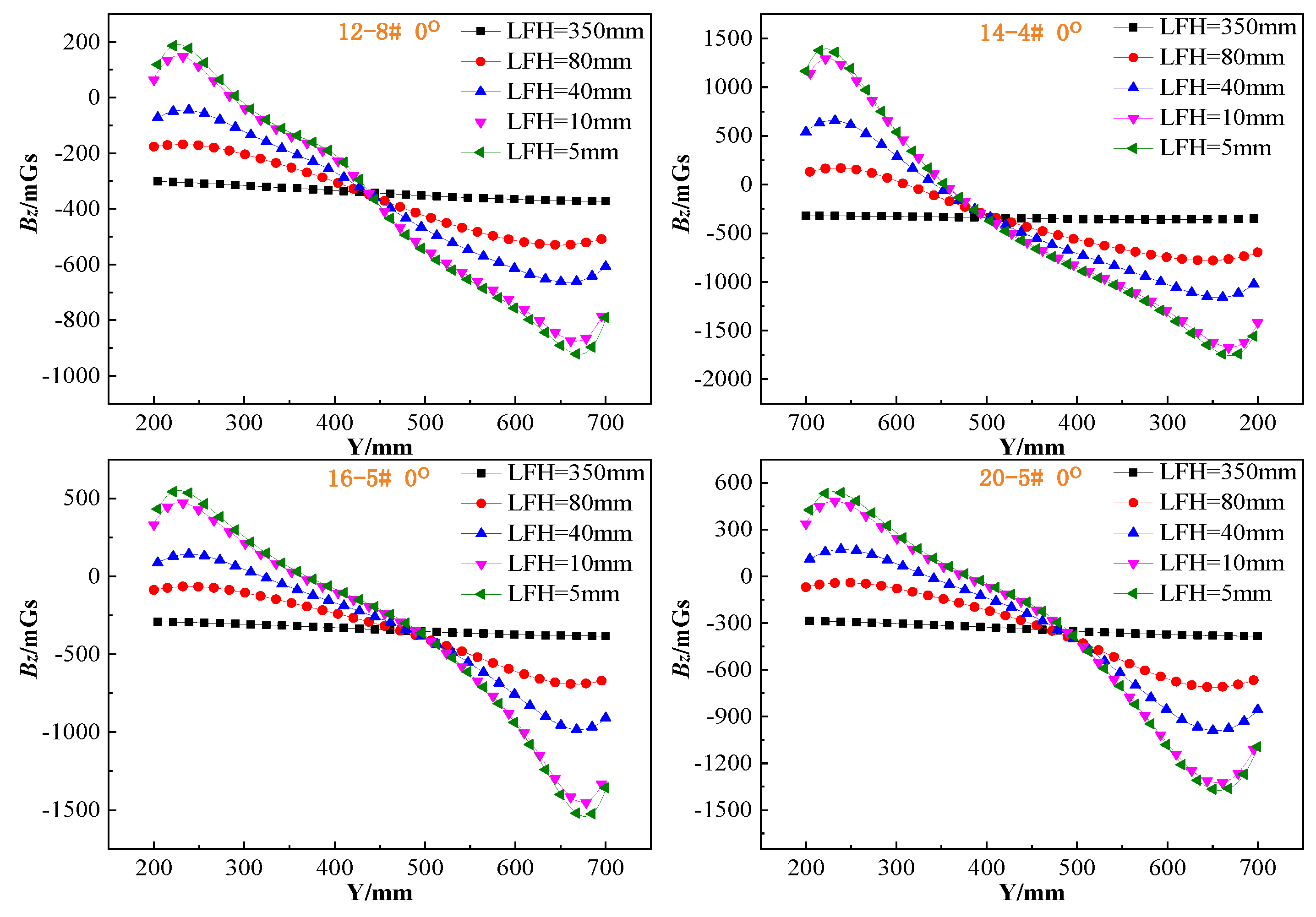
Experimental results for samples suggested that the SMFL signals at different angles of a certain steel bar were almost the same. Based on the magnetic dipole model, the SMFL field of a V-shaped defect can be represented. According to the B_Z component curves drawn by the experimental results, it was clear that the curves are different from the fluctuation of the uncorroded steel bar in the corrosion range. Therefore, corrosion was a major factor causing the change in B_Z curves.

(2)

SMFL is susceptible to magnetization history and initial magnetization state. In order to study the change of the SMFL signal separately, the geomagnetic field and the magnetic field of the steel bars were removed. It can be clearly seen that the curve gradient of B_Z in the corrosion region increases as the degree of corrosion increases. This observation supported the hypothesis that the variation gradient of the B_Z curve in the corroded region is related to the corrosion degree. An index “K” was introduced to estimate corrosion degree of steel bar. The index “K” was not affected by the magnetization history and the initial magnetization state. Finally, a SMFL-based quantitative analysis model for steel corrosion degree was established.

The present study achieved a quantitative analysis model for estimating the corrosion degree of steel bars. Further work is needed to fully explore the correlation between SMFL signals and a wide variety of corrosion defect shapes, such as trapezoid defect. There is, therefore, a definite need for the critical issues, such as the mathematical model correction and more samples, to validate the theoretical NDT method.

References

1. Gu, X.; Jin, X.; Yong, Z. Basic Principles of Concrete Structures, 3rd ed.; Tongji University Press: Shanghai, China, 2015; pp. 1–11. [Google Scholar]
2. An, L.; Ouyang, P.; Zheng, Y. Effect of stress concentration on mechanical properties of corroded steel bar bars. J. Southeast Uni. (Nat Sci. Ed.) 2005, 35, 940–944. [Google Scholar]
3. Li, H.; Wu, X.; Yue, J.J. Effect of corrosion pit position on mechanical properties of corroded HRB400 reinforced bar. Appl. Mech. Mater. 2015, 777, 220–223. [Google Scholar] [CrossRef]
4. Yuan, Y.; Ji, Y. Modeling corroded section configuration of steel bar in concrete structure. Constr. Build. Mater. 2009, 23, 2461–2466. [Google Scholar] [CrossRef]
5. Baby, S.; Balasubramanian, T.; Pardikar, R.J.; Palaniappan, M.; Subbaratnam, R. Time-of-flight diffraction (TOFD) technique for accurate sizing of surface-breaking cracks. Insight NDT Cond. Cond. Monit. 2003, 45, 600–604. [Google Scholar]
6. Soulioti, D.; Barkoula, N.M.; Paipetis, A.; Matikas, T.E.; Shiotani, T.; Aggelis, D.G. Acoustic emission behavior of steel fibre reinforced concrete under bending. Constr. Build. Mater. 2009, 23, 3532–3536. [Google Scholar] [CrossRef] [Green Version]
7. Logoń, D. Identification of the destruction process in quasi brittle concrete with dispersed fibers based on acoustic emission and sound spectrum. Materials 2019, 12, 2266. [Google Scholar] [CrossRef] [PubMed]
8. Du, G.; Wang, W.; Song, S.; Jin, S. Detection of corrosion on 304 stainless steel by acoustic emission measurement. Anti-Corros. Methods Mater. 2010, 57, 126–132. [Google Scholar] [CrossRef]
9. Lin, Z.B.; Azarmi, F.; Al-Kaseasbeh, Q.; Azimi, M.; Yan, F. Advanced ultrasonic testing technologies with applications to evaluation of steel bridge welding—An overview. Appl. Mech. Mater. 2015, 727–728, 785–789. [Google Scholar] [CrossRef]
10. Furuya, Y. Specimen size effects on gigacycle fatigue properties of high-strength steel under ultrasonic fatigue testing. Scr. Mater. 2008, 58, 1014–1017. [Google Scholar] [CrossRef]
11. Yeih, W.; Huang, R. Detection of the corrosion damage in reinforced concrete members by ultrasonic testing. Cem. Concr. Res. 1998, 28, 1071–1083. [Google Scholar] [CrossRef]
12. Rychkov, M.M.; Kaplin, V.V.; Malikov, E.L.; Smolyanskiy, V.A.; Stepanov, I.B.; Lutsenko, A.S.; Gentsel’man, V.; Vas’kovskiy, I.K. New microfocus bremsstrahlung source based on betatron B-18 for high-resolution radiofigurey and tomofigurey. In Proceedings of the IOP Conference Series: Materials Science and Engineering, Tomsk, Russia, 9 October 2018. [Google Scholar]
13. Schmidt, T.R. History of the remote-field eddy current inspection technique. Mater. Eval. 1989, 47, 14–22. [Google Scholar]
14. Ng, D.H.L.; Yu, C.C.; Li, A.S.K.; Lo, C.C.H. Measurement of Barkhausen emission and magnetoacoustic emission from a fractured steel bar. IEEE Trans. Magn. 2002, 31, 3394–3396. [Google Scholar] [CrossRef]
15. Dubov, A.A. A study of metal properties using the method of magnetic memory. Met. Sci. Heat Treat. 1997, 39, 401–405. [Google Scholar]
16. Park, D.G.; Ok, C.I.; Jeong, H.T.; Kuk, I.H.; Hong, J.H. Nondestructive evaluation of irradiation effects in RPV steel using Barkhausen noise and magnetoacoustic emission signals. J. Magn. Magn. Mater. 1999, 196–197, 382–384. [Google Scholar] [CrossRef]
17. Chen, L.; Que, P.-W.; Jin, T. A giant-magnetoresistance sensor for magnetic-flux-leakage nondestructive testing of a pipeline. Russ. J. Nondestr. Test. 2005, 41, 462–465. [Google Scholar]
18. Dong, L.H.; Xu, B.-s.; Dong, S.-y.; Chen, Q.-z.; Wang, Y.-y.; Zhang, L.; Wang, D.; Yin, D.-w. Metal magnetic memory testing for early damage assessment in ferromagnetic materials. J. Cent. S. Univ. 2005, 12, 102–106. [Google Scholar] [CrossRef]
19. Sawade, G.; Krause, H.J. 11-Magnetic flux leakage (MFL) for the non-destructive evaluation of pre-stressed concrete structures. In Non-Destructive Evaluation of Reinforced Concrete Structures; Woodhead Publishing: Cambridge, UK, 2010; pp. 215–242. [Google Scholar]
20. Pang, C.; Zhou, J.; Zhao, Q.; Zhao, R.; Chen, Z.; Zhou, Y. A new method for internal force detection of steel bars covered by concrete based on the metal magnetic memory effect. Metals 2019, 9, 661. [Google Scholar]
21. Zhang, H.; Liao, L.; Zhao, R.; Zhou, J.; Yang, M.; Xia, R. The non-destructive test of steel corrosion in reinforced concrete bridges using a micro-magnetic sensor. Sensors 2016, 16, 1439. [Google Scholar] [CrossRef]
22. Xia, R.; Zhou, J.; Zhang, H.; Liao, L.; Zhao, R.; Zhang, Z. Quantitative study on corrosion of steel strands based on self-magnetic flux leakage. Sensors 2018, 18, 1396. [Google Scholar] [CrossRef]
23. Qiu, J.; Zhang, H.; Zhou, J.; Ma, H.; Liao, L. Experimental analysis of the correlation between bending strength and SMFL of corroded RC beams. Constr. Build. Mater. 2019, 214, 594–605. [Google Scholar]
24. Qu, Y.; Zhang, H.; Zhao, R.; Liao, L.; Zhou, Y. Research on the Method of Predicting Corrosion width of Cables Based on the Spontaneous Magnetic Flux Leakage. Materials 2019, 12, 2154. [Google Scholar] [CrossRef] [PubMed]
25. Magistrali, G.; Giorcelli, C. Low frequency demagnetization of large diameter steel bars of high coercive force. J. Am. Stat. Assoc. 1982, 91, 1423–1431. [Google Scholar]
26. Stansbury, E.E.; Buchanan, R.A. Fundamentals of electrochemical corrosion. Avtomat I Telemekh. 2000, 309, 55–71. [Google Scholar]
27. Förster, F. Nondestructive inspection by the method of magnetic leakage fields: Theoretical and experimental foundations of the detection of surface cracks of finite and infinite depth. Sov. J. Nondestr. Test. 1982, 8, 841–859. [Google Scholar]
28. Zatsepin, N.N.; Shcherbinin, V.E. Calculation of the magnetostatic field of surface defects I. Field to pofigurey of defect models. Sov. J. Nondestr. Test. 1966, 5, 385–393. [Google Scholar]
29. Shur, M.L.; Zagidulin, R.V.; Shcherbinin, V.E. Theoretical problems of the field formation from a surface defect. Defektoskopiya 1988, 3, 14–25. [Google Scholar]
30. Zagidulin, R.V. Calculation of the remnant magnetic field of a discontinuity defect in a ferromagnetic sample. II. Remnant magnetic field of a defect in the air. Defektoskopiya 1998, 10, 33–39. [Google Scholar]
Figure 1. Calculation model of steel bars.
Metals 09 00952 g001
Figure 2. The layout of an experimental corrosion device.
Metals 09 00952 g002
Figure 3. The layout of the three-axis self-magnetic flux leakage (SMFL) scanning device.
Metals 09 00952 g003
Figure 4. The scanning paths of the magnetometer HMR2300: (a) Front view of the scanning paths; (b) Side view of the scanning paths.
Metals 09 00952 g004
Figure 5. The simplified model of a corroded steel bar.
Metals 09 00952 g005
Figure 6. The Hz curves calculated from Equation (9).
Metals 09 00952 g006
Figure 7. Experimental samples of steel bars.
Metals 09 00952 g007
Figure 8. BZ curves for steel bars with different diameters.
Metals 09 00952 g008
Figure 9. BZ curves for different angles of a steel bar.
Metals 09 00952 g009
Figure 10. The BZ curves of a sample 12-10#.
Metals 09 00952 g010
Figure 11. The correlation between α and G.
Metals 09 00952 g011
Figure 12. The correlation between α and G of all samples with LFH = 5 mm and 10 mm.
Metals 09 00952 g012
Figure 13. Parameters G and K of the samples 12-1#–12-10#: (a) α and G/G0; (b) α and K.
Metals 09 00952 g013
Figure 14. Correlation between α and K with LFH = 5 mm and 10 mm for all samples.
Metals 09 00952 g014