A New S-Shape Specimen for Studying the Dynamic Shear Behavior of Metals


Abstract
1. Introduction
2. Materials and Methods
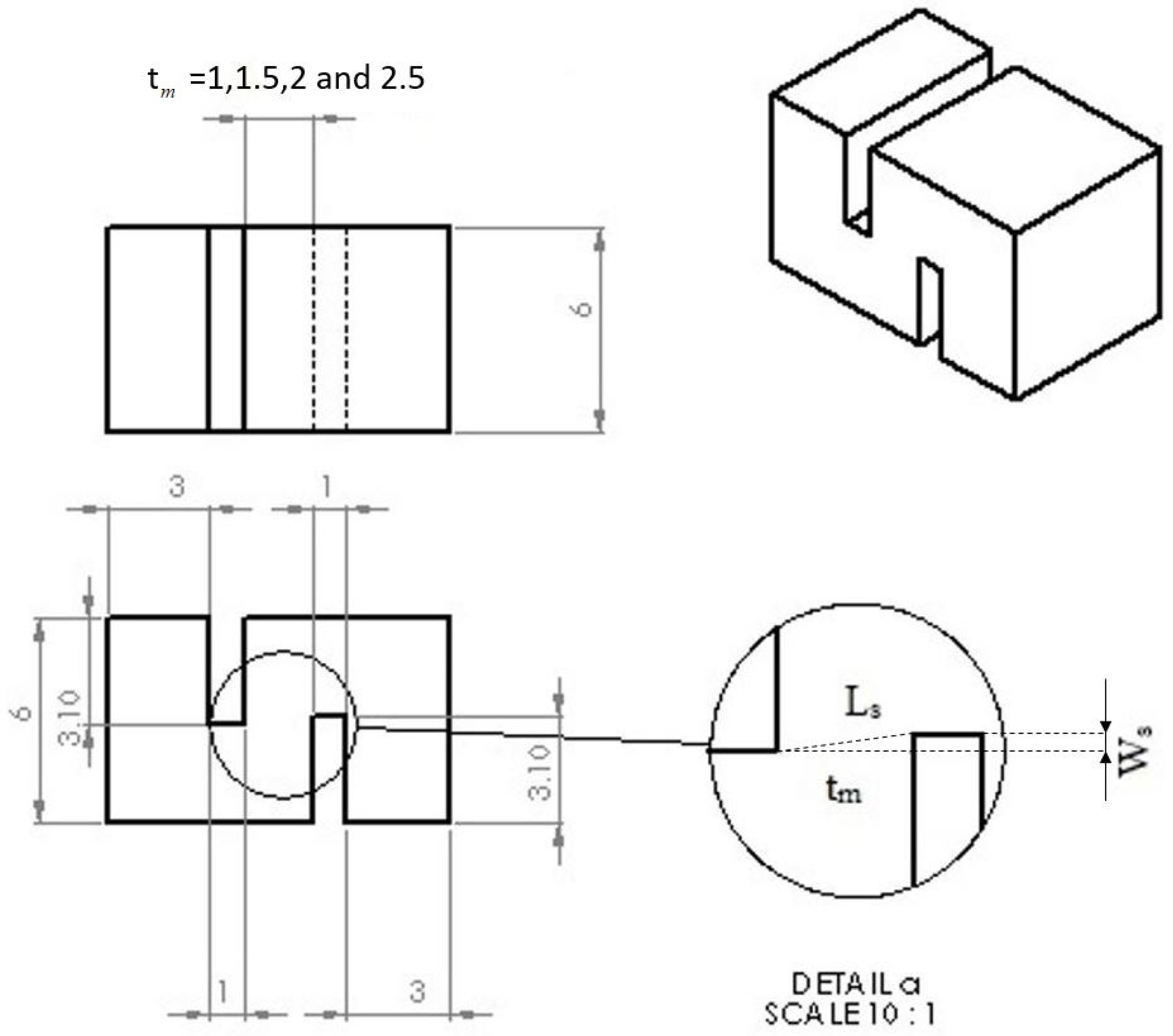
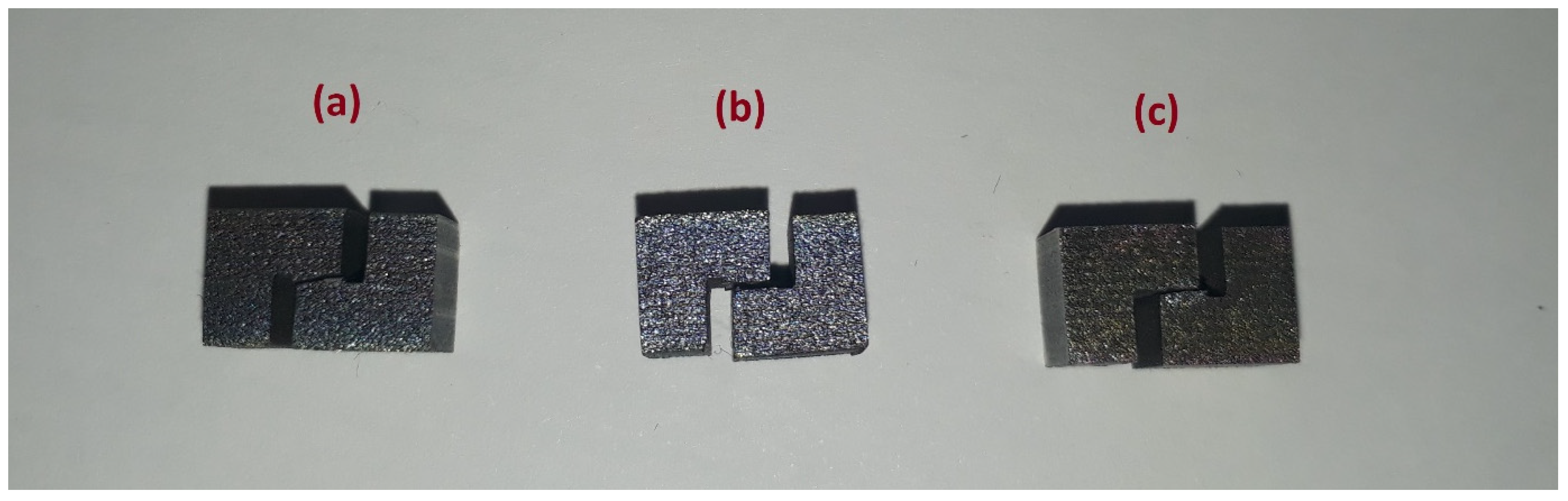
2.1. Materials and Specimens
2.2. DIC Measurement
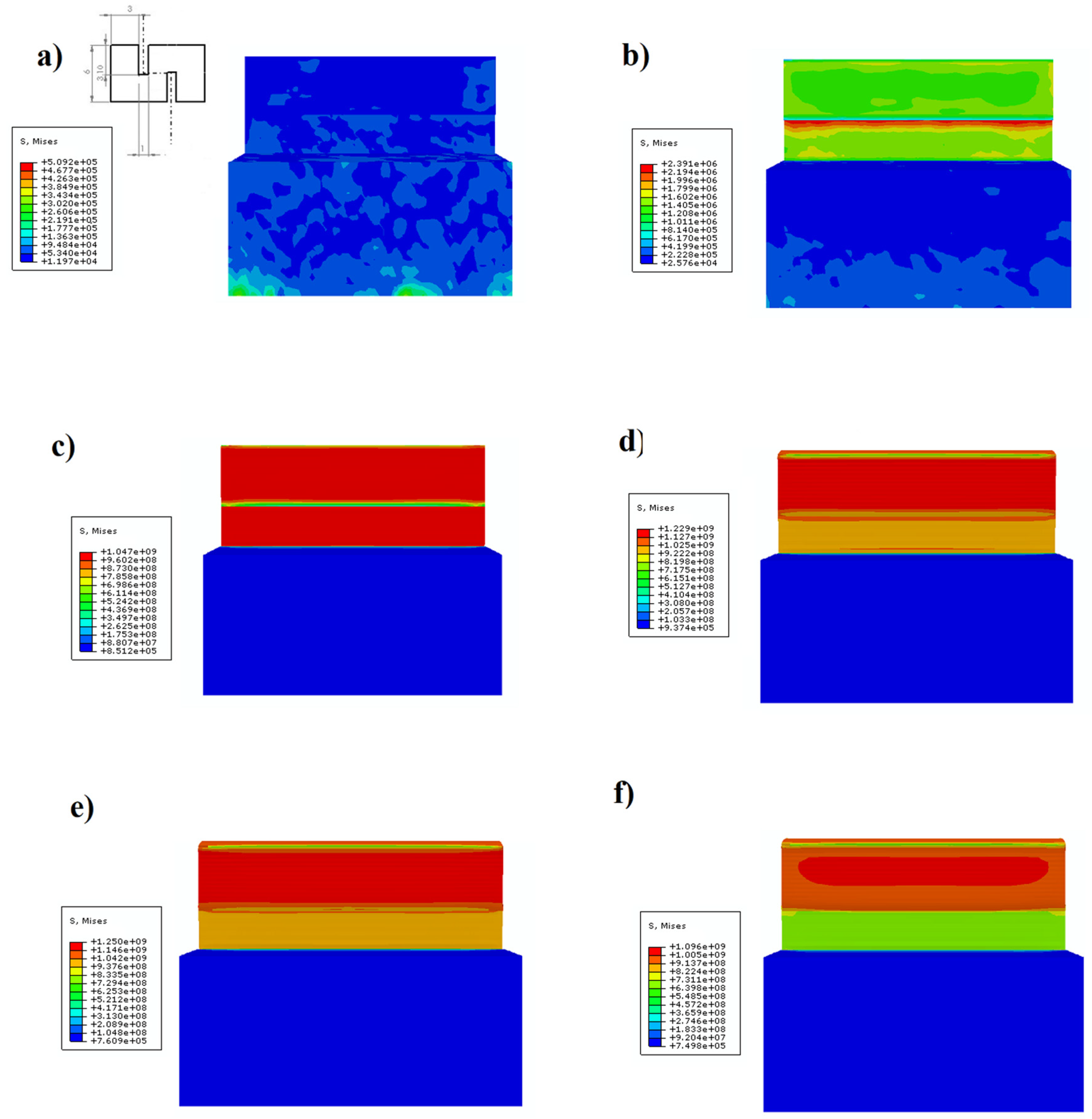
2.3. Finite Element Model (FEM) and Material Parameters
3. Results and Discussion
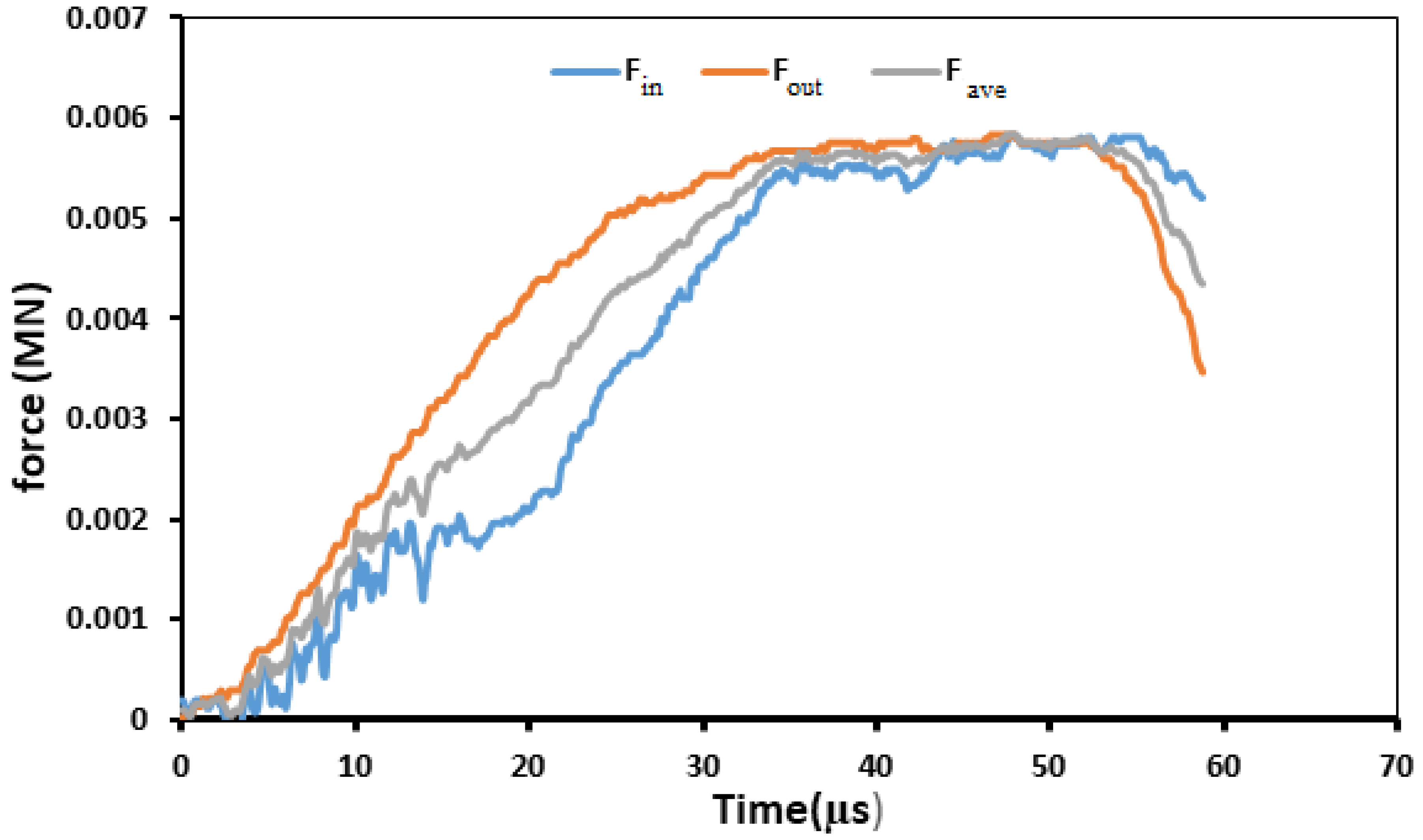
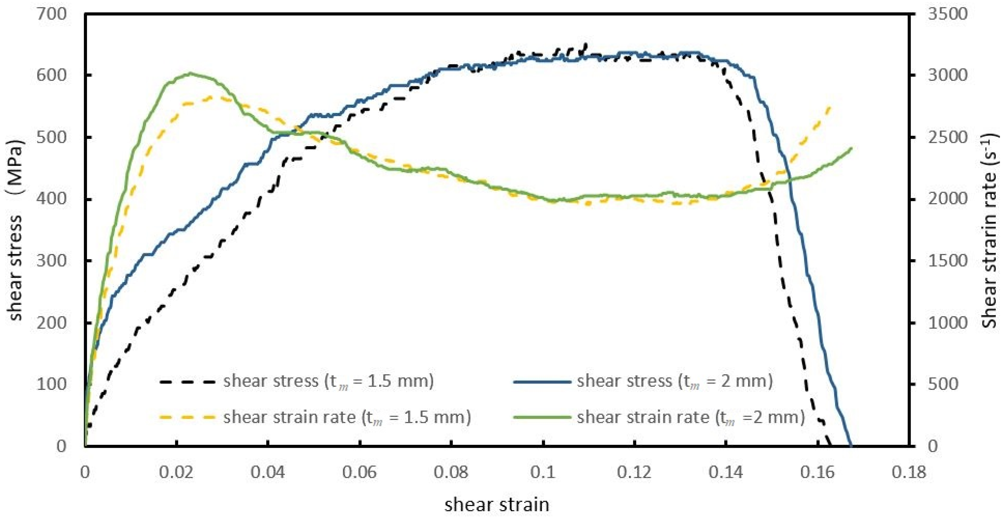
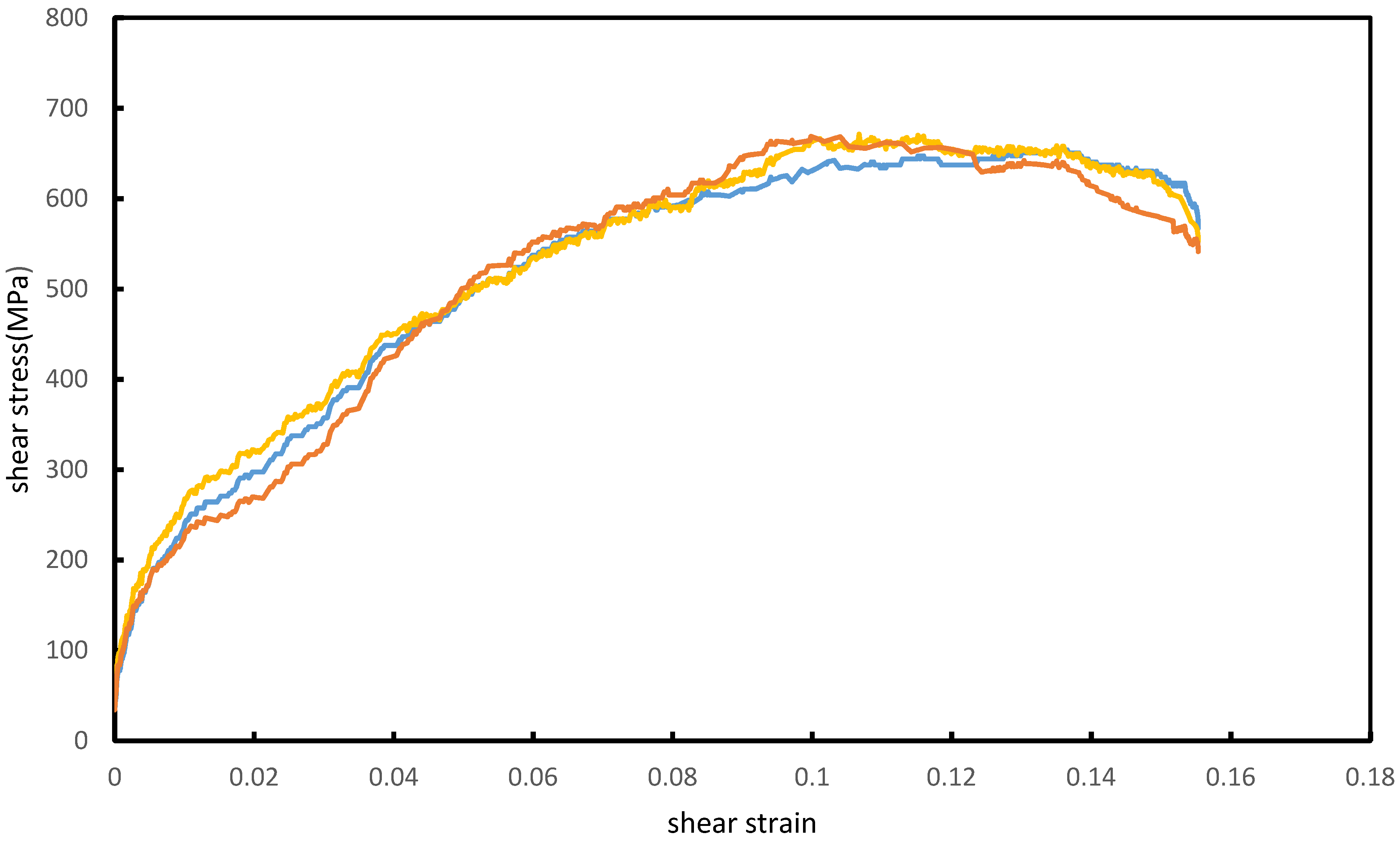
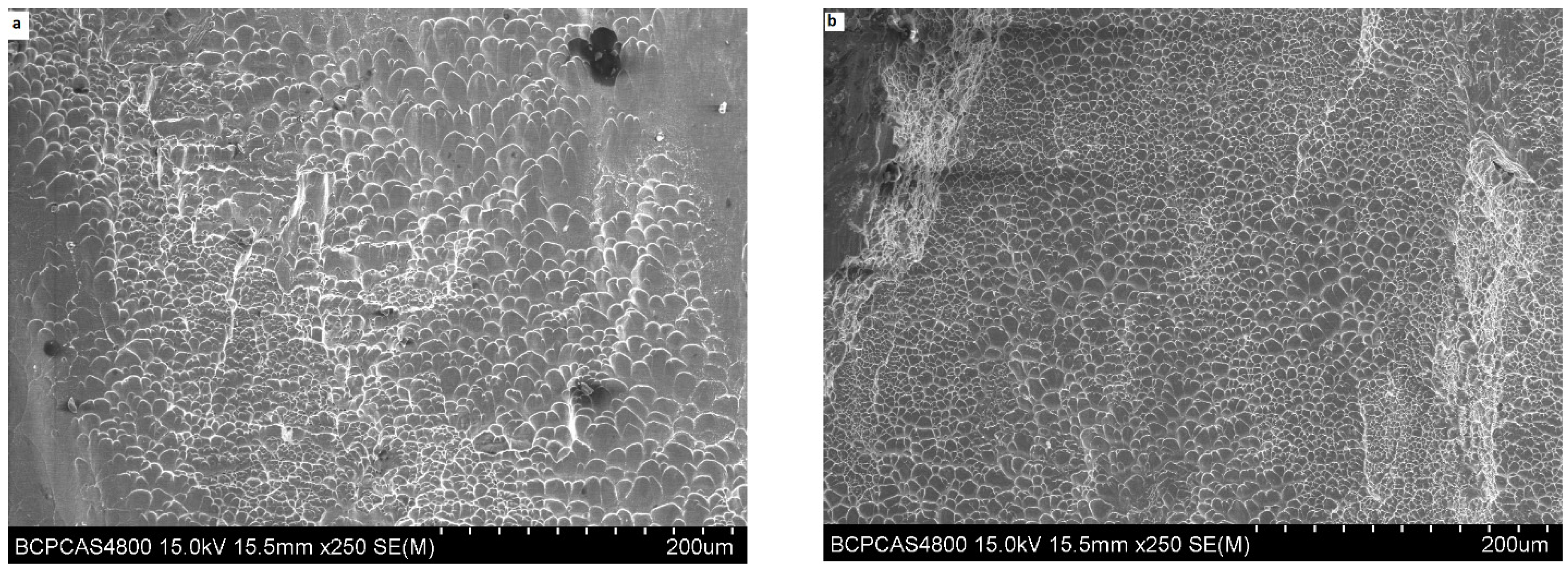
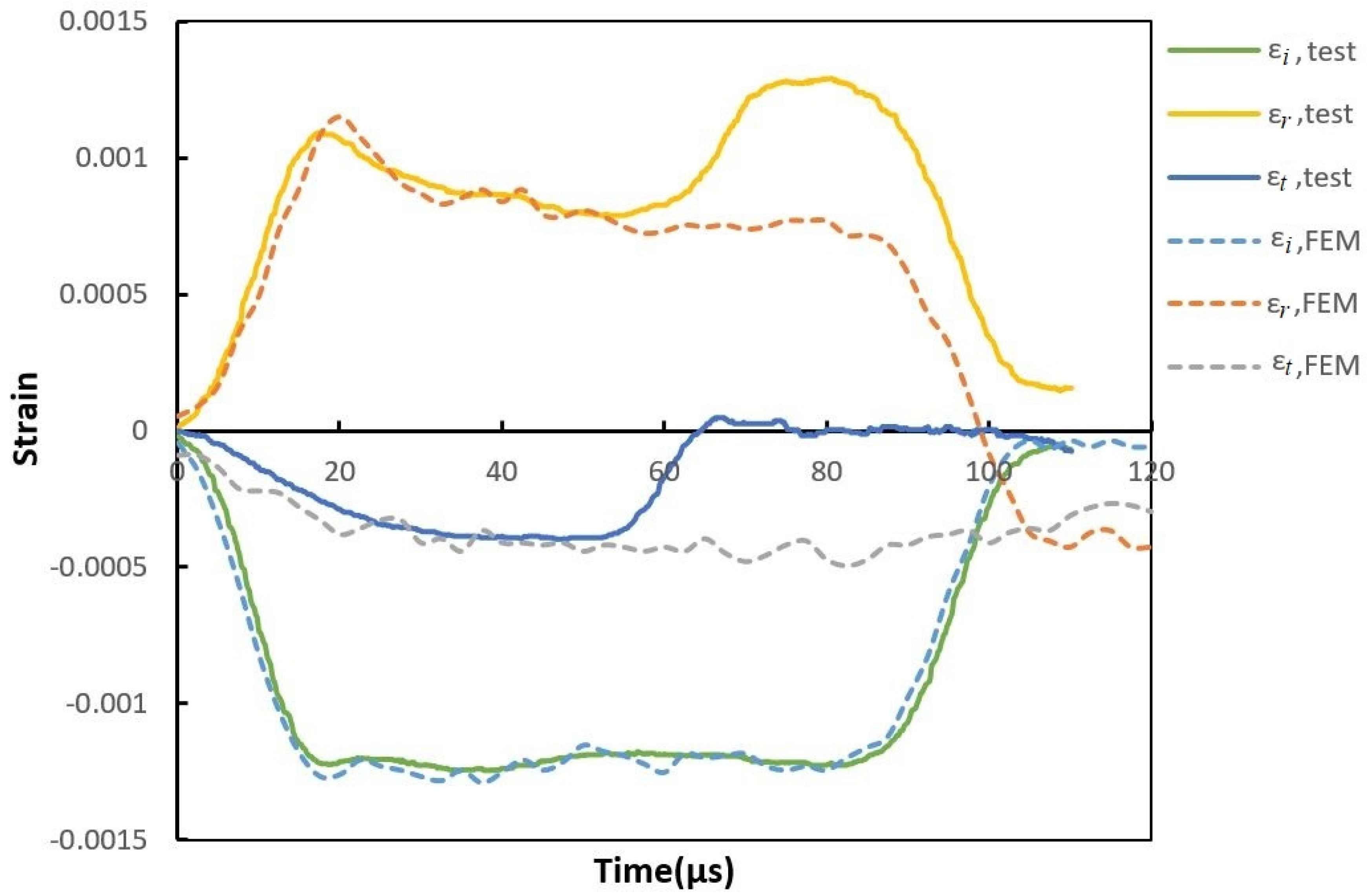
3.1. Dynamic Test (SHPB)
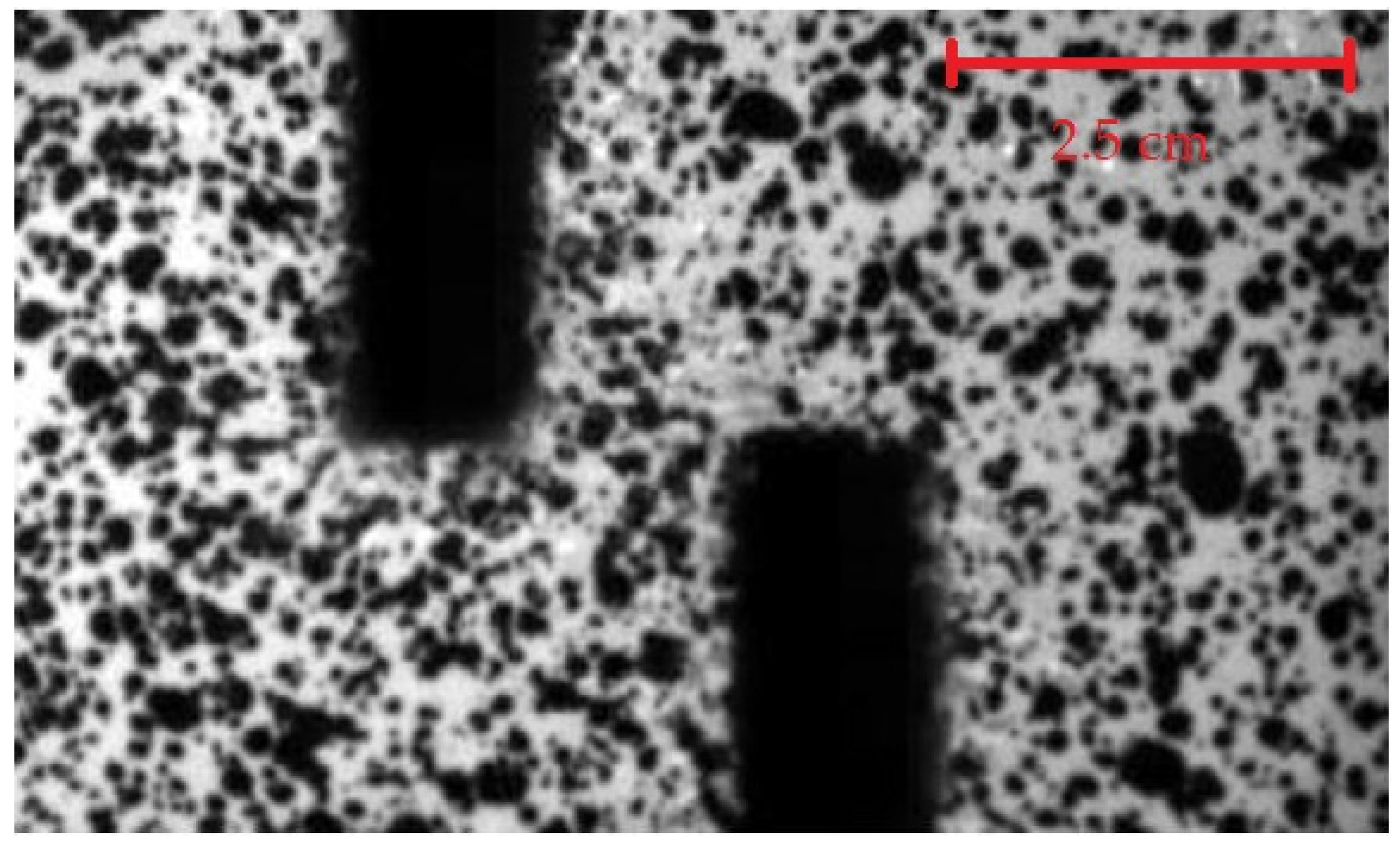
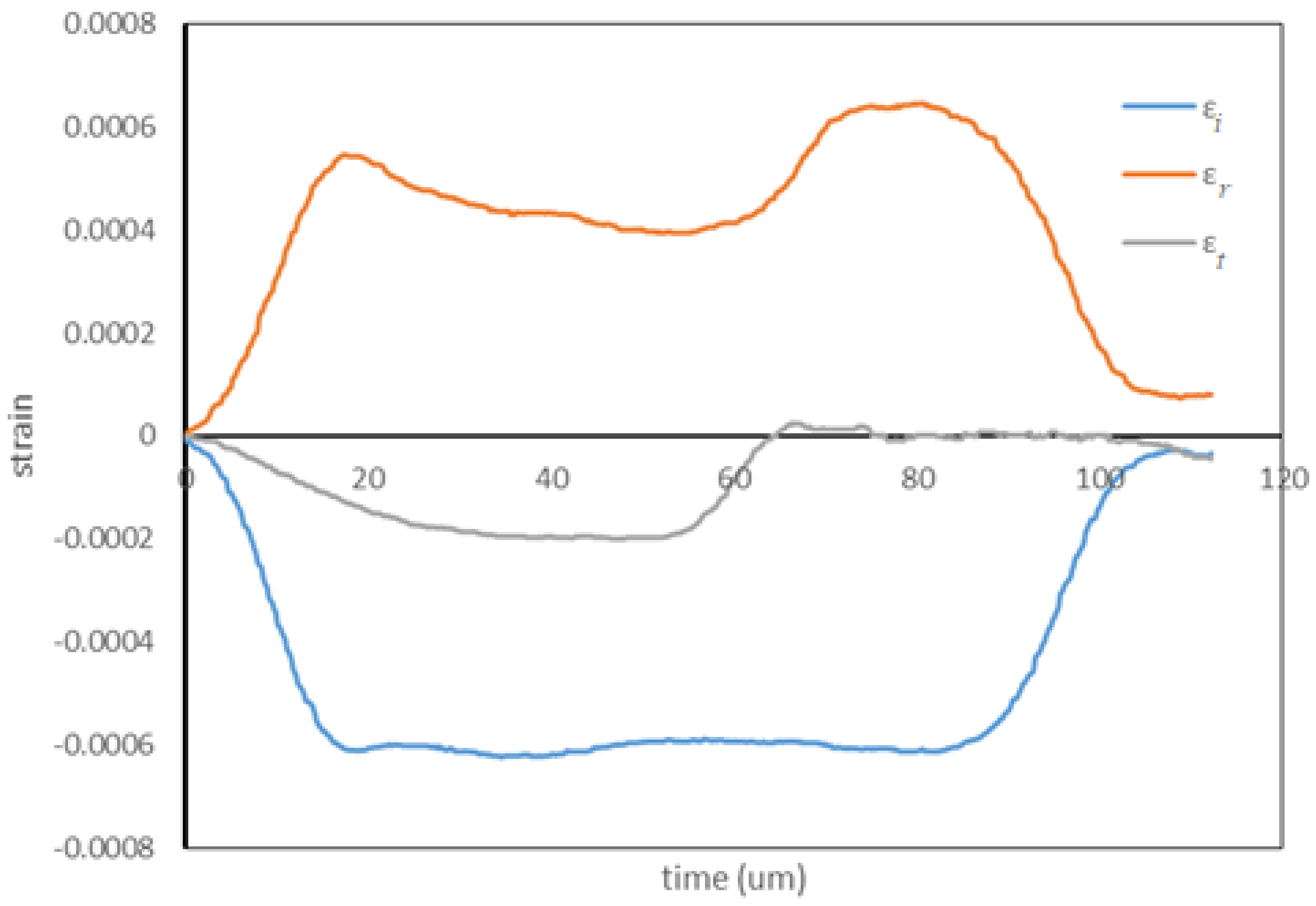
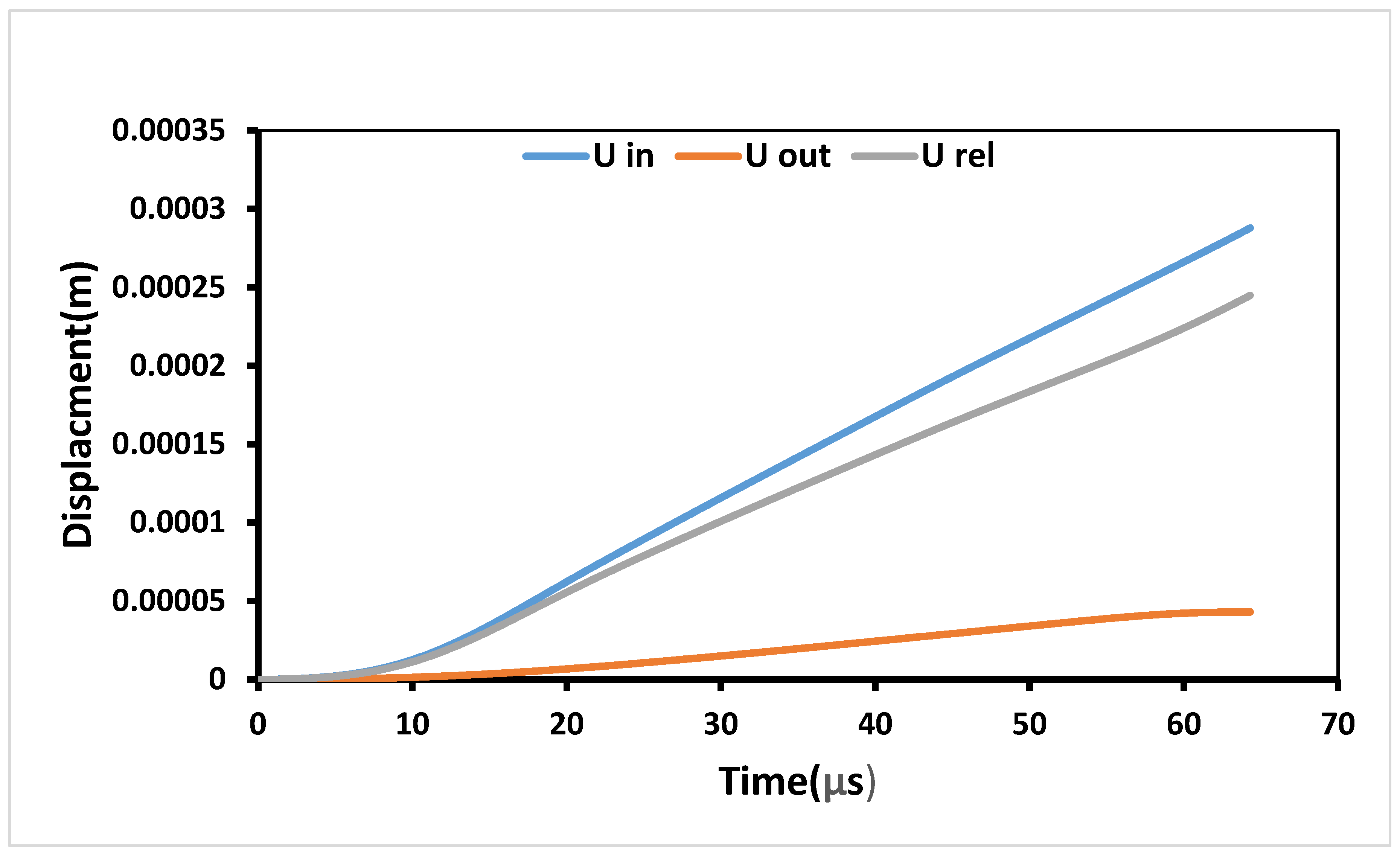
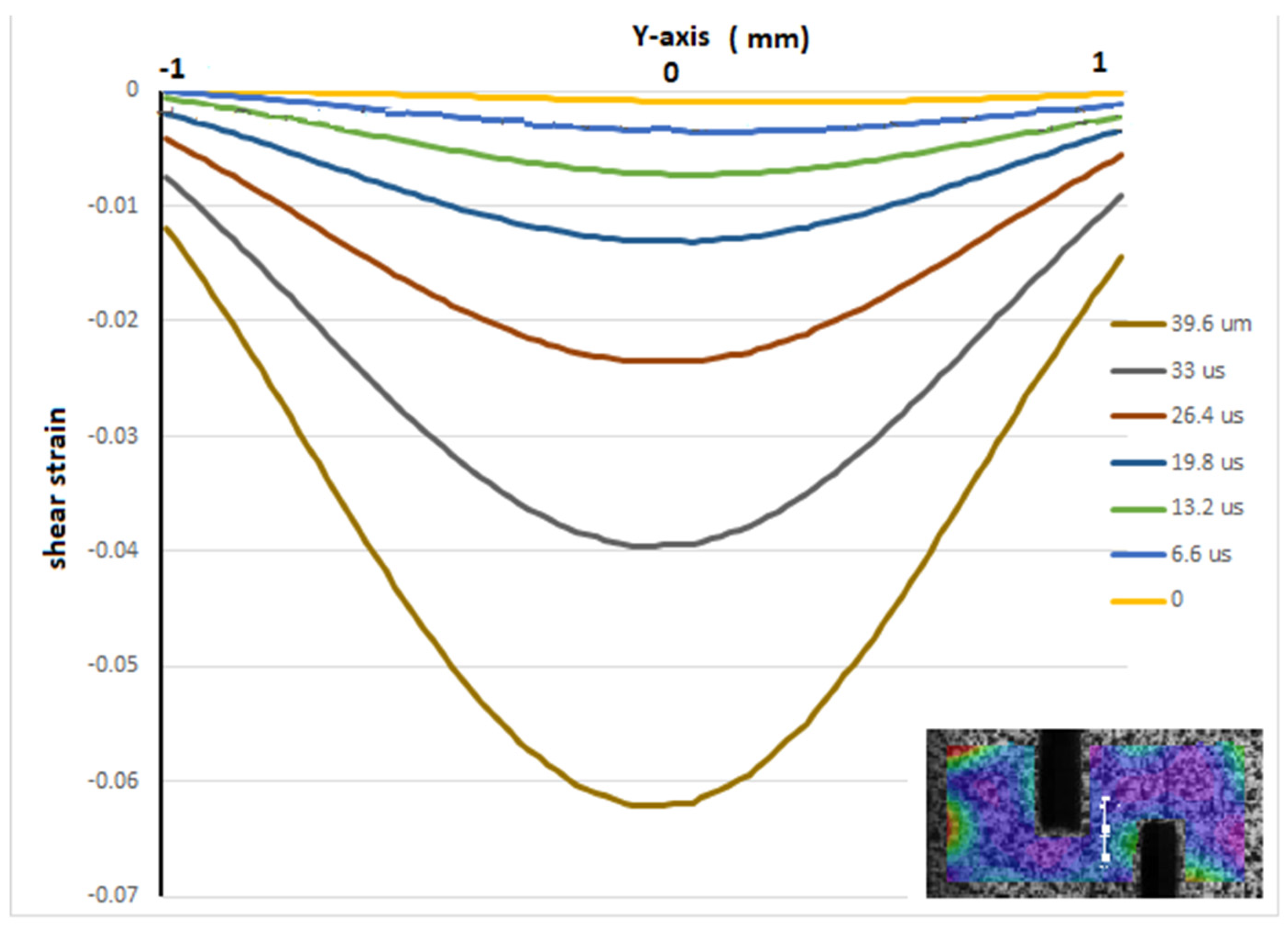
3.2. DIC
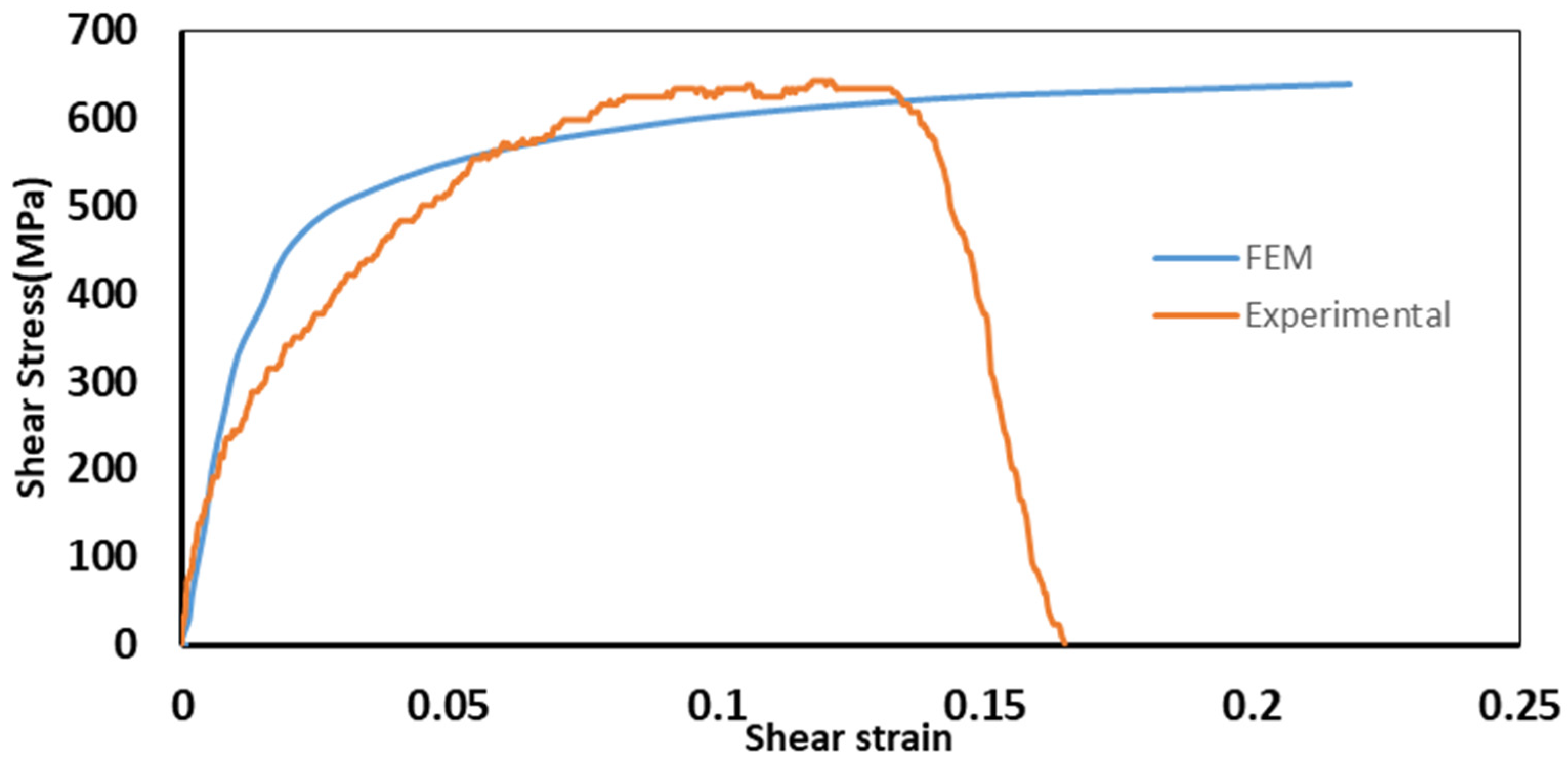
3.3. FEM Simulation
4. Conclusions
Author Contributions
Funding
Conflicts of Interest
References
- Peirs, J.; Verleysen, P.; Degrieck, J. Novel technique for static and dynamic shear testing of Ti6Al4V sheet. Exp. Mech. 2012, 52, 729–741. [Google Scholar] [CrossRef]
- Arab, A.; Chen, P.; Guo, Y. Effects of microstructure on the dynamic properties of TA15 titanium alloy. Mech. Mater. 2019, 137, 103121. [Google Scholar]
- Rittel, D.; Wang, Z.G.; Dorogoy, A. Geometrical imperfection and adiabatic shear banding. Int. J. Impact Eng. 2008, 35, 1280–1292. [Google Scholar] [CrossRef]
- Lins, J.F.C.; Sandim, H.R.Z.; Kestenbach, H.-J.; Raabe, D.; Vecchio, K.S. A microstructural investigation of adiabatic shear bands in an interstitial free steel. Mater. Sci. Eng. A 2007, 457, 205–218. [Google Scholar] [CrossRef]
- Zheng, C.; Wang, F.; Cheng, X.; Liu, J.; Liu, T.; Zhu, Z.; Yang, K.; Peng, M.; Jin, D. Capturing of the propagating processes of adiabatic shear band in Ti-6Al-4V alloys under dynamic compression. Mater. Sci. Eng. A 2016, 658, 60–67. [Google Scholar] [CrossRef]
- Zurek, A.K. The study of adiabatic shear band instability in a pearlitic 4340 steel using a dynamic punch test. Metall. Mater. Trans. A 1994, 25, 2483–2489. [Google Scholar] [CrossRef]
- Wang, B.F.; Yang, Y. Microstructure evolution in adiabatic shear band in fine-grain-sized Ti-3Al-5Mo-4.5V alloy. Mater. Sci. Eng. A 2008, 473, 306–311. [Google Scholar] [CrossRef]
- Wang, B.; Wang, X.; Li, Z.; Ma, R.; Zhao, S.; Xie, F.; Zhang, X. Shear localization and microstructure in coarse grained beta titanium alloy. Mater. Sci. Eng. A 2016, 652, 287–295. [Google Scholar] [CrossRef]
- Odeshi, A.G.; Bassim, M.N.; Al-Ameeri, S. Effect of heat treatment on adiabatic shear bands in a high-strength low alloy steel. Mater. Sci. Eng. A 2006, 419, 69–75. [Google Scholar] [CrossRef]
- Klepaczko, J.R. An experimental technique for shear testing at high and very high strain rates. The case of a mild steel. Int. J. Impact Eng. 1994, 15, 25–39. [Google Scholar] [CrossRef]
- Xu, Z.; Ding, X.; Zhang, W.; Huang, F. A novel method in dynamic shear testing of bulk materials using the traditional SHPB technique. Int. J. Impact Eng. 2017, 101, 90–104. [Google Scholar] [CrossRef]
- Lindholm, U.S.; Johnson, G.R. Strain-rate effects in metals at large shear strains. In Material Behavior Under High Stress and Ultrahigh Loading Rates, Mescall, J.; Weiss, W., Ed.; Springer: Boston, MA, USA, 1983; pp. 61–79. [Google Scholar]
- Ran, C.; Chen, P.; Li, L.; Zhang, W.; Liu, Y.; Zhang, X. High-strain-rate plastic deformation and fracture behaviour of Ti-5Al-5Mo-5V-1Cr-1Fe titanium alloy at room temperature. Mech. Mater. 2018, 116, 3–10. [Google Scholar] [CrossRef]
- Ran, C.; Chen, P.; Li, L.; Zhang, W. Dynamic shear deformation and failure of Ti-5Al-5Mo-5V-1Cr-1Fe titanium alloy. Mater. Sci. Eng. A 2017, 694, 41–47. [Google Scholar] [CrossRef]
- Rittel, D.; Lee, S.; Ravichandran, G. A shear-compression specimen for large strain testing. Exp. Mech. 2002, 42, 58–64. [Google Scholar] [CrossRef]
- Dorogoy, A.; Rittel, D. Numerical validation of the shear compression specimen. Part I: quasi-static large strain testing. Exp. Mech. 2005, 45, 167–177. [Google Scholar] [CrossRef]
- Dorogoy, A.; Rittle, D. Numerical validation of the shear testing, specimen. Part II: dynamic large strain. Exp. Mech. 2005, 45, 178–185. [Google Scholar] [CrossRef]
- Guo, Y.; Li, Y. A novel approach to testing the dynamic shear response of Ti-6Al-4V. Acta Mech. Solida Sin. 2012, 25, 299–311. [Google Scholar] [CrossRef]
- Gray, G.T.; Vecchio, K.S.; Livescu, V. Compact forced simple-shear sample for studying shear localization in materials. Acta Mater. 2016, 103, 12–22. [Google Scholar] [CrossRef]
- Peirs, J.; Verleysen, P.; Degrieck, J.; Coghe, F. The use of hat-shaped specimens to study the high strain rate shear behaviour of Ti-6Al-4V. Int. J. Impact Eng. 2010, 37, 703–714. [Google Scholar] [CrossRef]
- Jiang, Y.; Chen, Z.; Zhan, C.; Chen, T.; Wang, R.; Liu, C. Adiabatic shear localization in pure titanium deformed by dynamic loading: Microstructure and microtexture characteristic. Mater. Sci. Eng. A 2015, 640, 436–442. [Google Scholar] [CrossRef]
- Ma, Y.; Yuan, F.; Yang, M.; Jiang, P.; Ma, E.; Wu, X. Dynamic shear deformation of a CrCoNi medium-entropy alloy with heterogeneous grain structures. Acta Mater. 2018, 148, 407–418. [Google Scholar] [CrossRef]
- Meyer, L.W.; Halle, T. Shear strength and shear failure, overview of testing and behavior of ductile metals. Mech. Time-Dependent Mater. 2011, 15, 327–340. [Google Scholar] [CrossRef]
- Ran, C.; Chen, P. Dynamic shear deformation and failure of Ti-6Al-4V and Ti-5Al-5Mo-5V-1Cr-1Fe alloys. Materials 2018, 11, 76. [Google Scholar] [CrossRef]
- Sutton, M.A.; Orteu, J.-J.; Schreier, H.W. Image Correlation for Shape, Motion and Deformation Measurements: Basic Concepts, Theory and Applications; Springer Science & Business Media: New York, NY, USA, 2009. [Google Scholar]
- Huimin, P.B.X. Full-field strain measurement based on least-square fitting of local displacement for digital image correlation method. Acta Opt. Sin. 2007, 11, 014. [Google Scholar]
- Dorogoy, A.; Rittel, D. Determination of the johnson-cook material parameters using the SCS specimen. Exp. Mech. 2009, 49, 881–885. [Google Scholar] [CrossRef]
- Wang, B.; Liu, Z. Shear localization sensitivity analysis for Johnson-Cook constitutive parameters on serrated chips in high speed machining of Ti6Al4V. Simul. Model. Pract. Theory 2015, 55, 63–76. [Google Scholar] [CrossRef]
- Gama, B.A.; Lopatnikov, S.L.; Gillespie, J.W. Hopkinson bar experimental technique: A critical review. Appl. Mech. Rev. 2004, 57, 223. [Google Scholar] [CrossRef]
- Verleysen, P.; Peirs, J. Quasi-static and high strain rate fracture behaviour of Ti6Al4V. Int. J. Impact Eng. 2016, 000, 1–19. [Google Scholar] [CrossRef]
- Osovski, S.; Nahmany, Y.; Rittel, D.; Landau, P.; Venkert, A. On the dynamic character of localized failure. Scr. Mater. 2012, 67, 693–695. [Google Scholar] [CrossRef]
- Rittel, D.; Wang, Z.G. Thermo-mechanical aspects of adiabatic shear failure of AM50 and Ti6Al4V alloys. Mech. Mater. 2008, 40, 629–635. [Google Scholar] [CrossRef]
- Zhang, J.; Tan, C.-W.; Ren, Y.; Yu, X.-D.; Ma, H.-L.; Wang, F.-C.; Cai, H.-N. Adiabatic shear fracture in Ti-6Al-4V alloy. Trans. Nonferrous Met. Soc. China 2011, 21, 2396–2401. [Google Scholar] [CrossRef]
- Tiwari, V.; Sutton, M.A.; Shultis, G.; McNeill, S.R.; Xu, S.; Deng, X.; Fourney, W.L.; Bretall, D. Measuring full-field transient plate deformation using high speed imaging systems and 3D DIC. Soc. Exp. Mech. SEM Annu. Conf. Expo. Exp. Appl. Mech. 2009, 1, 481–488. [Google Scholar]
- Gao, G.; Huang, S.; Xia, K.; Li, Z. Application of digital image correlation (DIC) in dynamic notched semi-circular bend (NSCB) tests. Exp. Mech. 2015, 55, 95–104. [Google Scholar] [CrossRef]


| Part | Material | Density, kg/m3 | Elastic Modulus, E (GPa) | Poisson’s Ratio | Specific Heat, Cp (J/kg °C) | Tmelt, (K) | Troom (K) |
|---|---|---|---|---|---|---|---|
| Specimen | Ti-6Al-4V | 4300 | 110 | 0.33 | 670 | 1903 | 298 |
| Bar | Steel | 7800 | 190 | 0.33 | -- | -- | -- |
| Set | A (MPa) | B (MPa) | N | C | m | |
|---|---|---|---|---|---|---|
| J–C | 862 | 331 | 0.34 | 0.012 | 0.8 | 1 |
© 2019 by the authors. Licensee MDPI, Basel, Switzerland. This article is an open access article distributed under the terms and conditions of the Creative Commons Attribution (CC BY) license (http://creativecommons.org/licenses/by/4.0/).
Share and Cite
Arab, A.; Guo, Y.; Zhou, Q.; Chen, P. A New S-Shape Specimen for Studying the Dynamic Shear Behavior of Metals. Metals 2019, 9, 838. https://doi.org/10.3390/met9080838
Arab A, Guo Y, Zhou Q, Chen P. A New S-Shape Specimen for Studying the Dynamic Shear Behavior of Metals. Metals. 2019; 9(8):838. https://doi.org/10.3390/met9080838
Chicago/Turabian StyleArab, Ali, Yansong Guo, Qiang Zhou, and Pengwan Chen. 2019. "A New S-Shape Specimen for Studying the Dynamic Shear Behavior of Metals" Metals 9, no. 8: 838. https://doi.org/10.3390/met9080838
APA StyleArab, A., Guo, Y., Zhou, Q., & Chen, P. (2019). A New S-Shape Specimen for Studying the Dynamic Shear Behavior of Metals. Metals, 9(8), 838. https://doi.org/10.3390/met9080838