Detecting and Monitoring Cracks in Aerospace Materials Using Post-Processing of TSA and AE Data

Abstract

Thermoelastic stress analysis (TSA) is a non-contact technique for measuring the distribution of stress in the surface of a component subject to cyclic loading by using a sensitive infrared camera. The stress concentrations indicative of a crack can be located and tracked using an optical flow method, allowing the position of the crack-tip to be identified at a given time. Acoustic emission (AE) has been used to validate the TSA algorithm. AE events from cracking, located using the Delta-T Mapping method, were detected several seconds before the TSA algorithm first detected cracking; however, TSA provided significantly more accurate location information.

1. Introduction

The early detection and subsequent monitoring of damage in engineering structures is important, as it allows remedial measures such as repair, replacement or redesign to occur. A variety of non-destructive testing (NDT) methods exist which are currently used in laboratory or industrial testing, such as visual inspection, thermoelastic stress analysis (TSA), acoustic emission (AE), digital image correlation (DIC), electronic speckle pattern interferometry (ESPI), electrical resistance and strain gauges [1,2,3]. These methods include contact and non-contact techniques and range from point measurements (e.g., strain gauges) to full-field measurements (e.g., TSA, DIC) [1,2].

In previous work, it has been shown that TSA data can be used to observe the changes in the surface stress distribution in a component during initiation of a crack, and its subsequent propagation [4,5,6], with some studies working towards automated tracking of artificially induced cracks [7,8]. In new research in the EU H2020 INSTRUCTIVE project, an optical flow algorithm has been developed and used to automatically detect the presence of a naturally initiating crack and to locate its tip using TSA data [9]. Experiments have demonstrated that the new algorithm can detect cracks of the order of 1 mm long and can track the crack growth to failure of the component. Cracks of the order of 1 mm length are not readily visible to the naked eye and would not be found in a routine visual inspection of a structure. Traditionally, a matt black paint has been applied to surfaces prior to performing TSA in order to provide a uniform emissivity; however, tests have shown that the epoxy-based primer used widely in the aerospace industry provides an excellent surface finish for TSA [9,10].

Acoustic emission is the transient elastic energy released as a material undergoes a change in its internal structure, such as plastic deformation or cracking [11]. The energy released from these events travels through the structure as a stress wave, which can be detected by piezoelectric AE sensors bonded to the structure’s surface. AE lends itself well to damage detection for structural health monitoring (SHM) purposes due to its passive nature and ability to conduct global monitoring in situ. One of the other major benefits of AE is its ability to locate detected signals through the use of an array of sensors. The differences in time of arrival of a detected signal at each of the recording sensors can be used in a form of triangulation to calculate the location of the source; this is known as Time of Arrival (TOA) location [12]. However, the traditional TOA method makes a number of simplifying assumptions which reduce its accuracy in non-isotropic materials or in structures with geometric irregularities, such as holes. In order to improve upon this, a bespoke location algorithm known as Delta-T Mapping was developed at Cardiff University [13], which has been shown to give more accurate source locations than the traditional TOA method [14,15]. A full description of Delta-T Mapping is available [16], though in short it involves the collection of training data prior to loading the structure which is to be monitored. The training data allow for the creation of maps of the difference in time of arrival of signals, originating from various points on the structure, between each of the pairs of sensors. The differences in time of arrival between real signals for sensor pairs recorded from testing can then be compared with these maps in order to identify their origin.

Due to the different preparation and equipment required for each monitoring system, there are certain advantages and limitations to the use of particular techniques. Here, a combination of contact, AE, and non-contact, TSA, methods are used to monitor the initiation and propagation of a fatigue crack in a simple metallic specimen, allowing a comparison between the results from two techniques.

2. Methods

Hole-in-plate specimens were manufactured from a sheet of aluminium alloy 2024-T3 of thickness 1.6 mm. The width of the specimens was 40 mm, length 200 mm, with a central hole of diameter 6 mm. This geometry results in stress concentrations around this central hole during loading, from which a fatigue crack could initiate naturally at an unknown position on the edge of the hole [9].

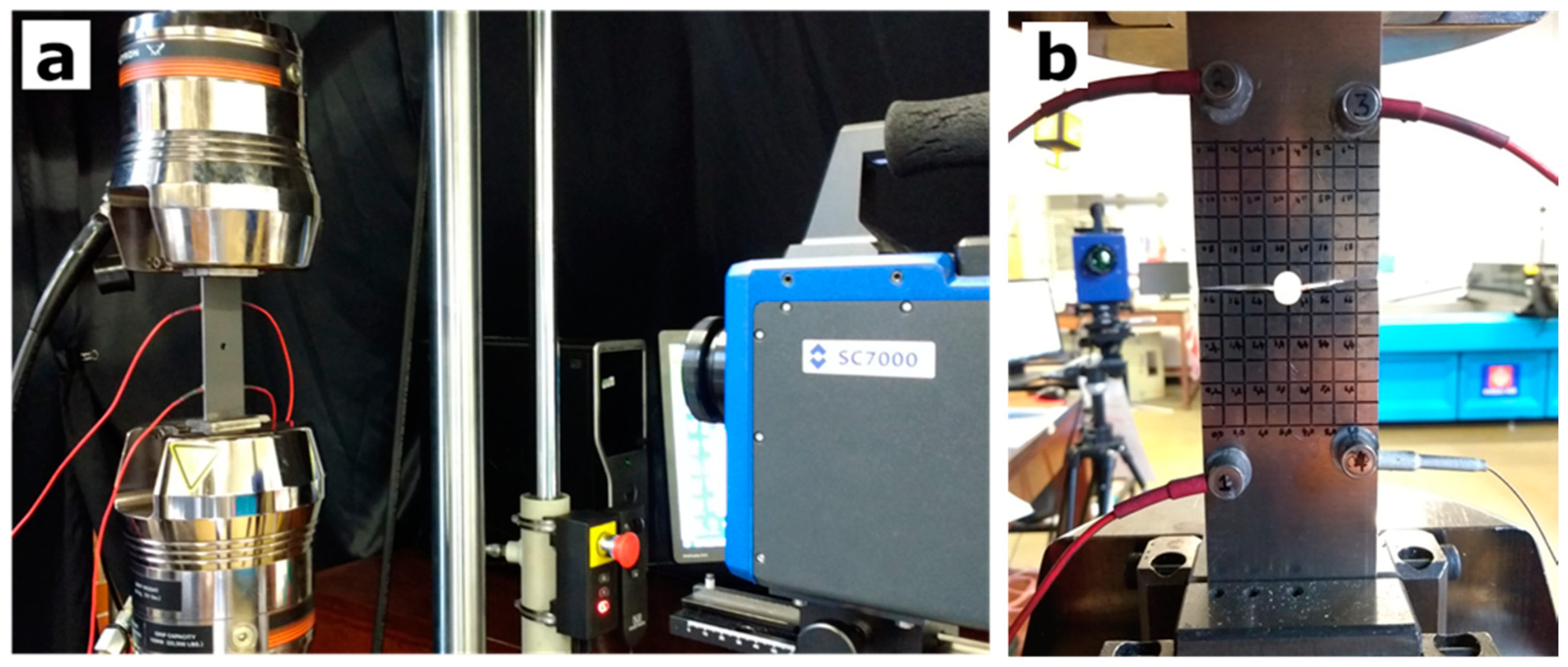
Four AE sensors (Nano 30; MISTRAS Group, Inc., Cambridge, UK) were bonded to the back of the specimens, as shown in Figure 1b, using silicone sealant (Loctite 595), which also served as the acoustic couplant between the sensors and the specimen. Once bonded, a Hsu-Neilson sensitivity test was conducted to ensure adequate coupling, with all sensors recording 99 dB responses [17].

For the purpose of AE event location using the Delta-T Mapping method [16], a distinction should be made here, between a “hit”: any signal crossing the threshold recorded by a sensor, and an “event”: a collection of hits which, due to their similarity in arrival time, are all deemed to have been produced by the same source. An AE event can be located when hits register on at least three sensors; however, a larger number of sensors allows a larger number of sensor pairs to be interrogated during Delta-T Mapping, and will improve the accuracy of the event location [14]. Here, the upper limit of sensor number was constrained by the acquisition system to four. The asymmetric sensor positioning, shown in Figure 1, was selected intentionally to avoid symmetry in the maps of difference in time of arrival between sensor pairs, as symmetry has been found to increase the likelihood of finding multiple crossing points in the Delta-T Mapping process and thus calculate erroneous location results [18].

The sensors were connected to a four-channel acquisition system (MISTRAS Group, Inc. PCI2 AEWin, Cambridge, UK) through 40 dB preamplifiers with a built-in 20–1200 kHz filter. AE hit recording was set up with peak definition, hit definition, and hit lockout times of 200, 200, and 1000 microseconds respectively; and detected hits were saved as waveforms with a 5 MHz sampling frequency. A 30 × 60 mm training grid was drawn on to the back surface of the specimen (Figure 1), centred around the hole. A grid with a 5 mm pitch was used based on previous experimentation into the effect of the grid pitch on the accuracy of the location results with Delta-T Mapping [15]. Artificial AE sources in the form of pencil lead-breaks, known as Hsu-Neilson sources [19], were generated at each grid point. These training data allowed the creation of the Delta-T maps that were subsequently used to calculate the location of AE occurring during the test.

In order to test the accuracy of the AE setup with Delta-T Mapping, a preliminary location study was conducted. Eight pseudo-random positions in the area of the training grid were selected and five Hsu-Neilson sources were generated at each. The location of these events, as calculated by Delta-T Mapping, was compared with the known location of the source; thus, a distance error for each event was calculated. The average error in location across all of the trial locations was 1.71 mm with a standard deviation of 1.06 mm.

The front of the specimen was coated with a thin layer of graphite (Graphit33; Kontakt Chemie, Iffezheim, Germany) and then loading was carried out under tension–tension cyclic conditions with F_max = 11.62 kN and F_min = 1.162 kN, at a frequency of 13 Hz. Data were collected simultaneously from the TSA system and AE systems until the specimen failed (Figure 1).

TSA data were collected with a high resolution, high sensitivity DeltaTherm 1780 system (Stress Photonics, Madison, WI, USA). TSA signal magnitude data were normalised, then datasets were analysed using the optical flow method detailed in Middleton et al. [9]. This method compares successive datasets to find changes in the stress distribution indicative of the crack, determining when the crack initiates and where the corresponding crack-tip is at a given time. AE hits were recorded with the same timing parameters as those used in the collection of the training data, though due to the presence of electrical noise it was necessary to use a threshold of 55 dB. Once the specimen had failed, the AE hits and associated waveforms were post-processed using Delta-T Mapping to determine the location of events. Only located AE events (i.e., sources which were detected on three or more sensors) were considered during further analysis in order to ensure that the AE investigated was generated due to crack development and that any potential source of noise, such as friction at the clamps, could be excluded.

3. Results and Discussion

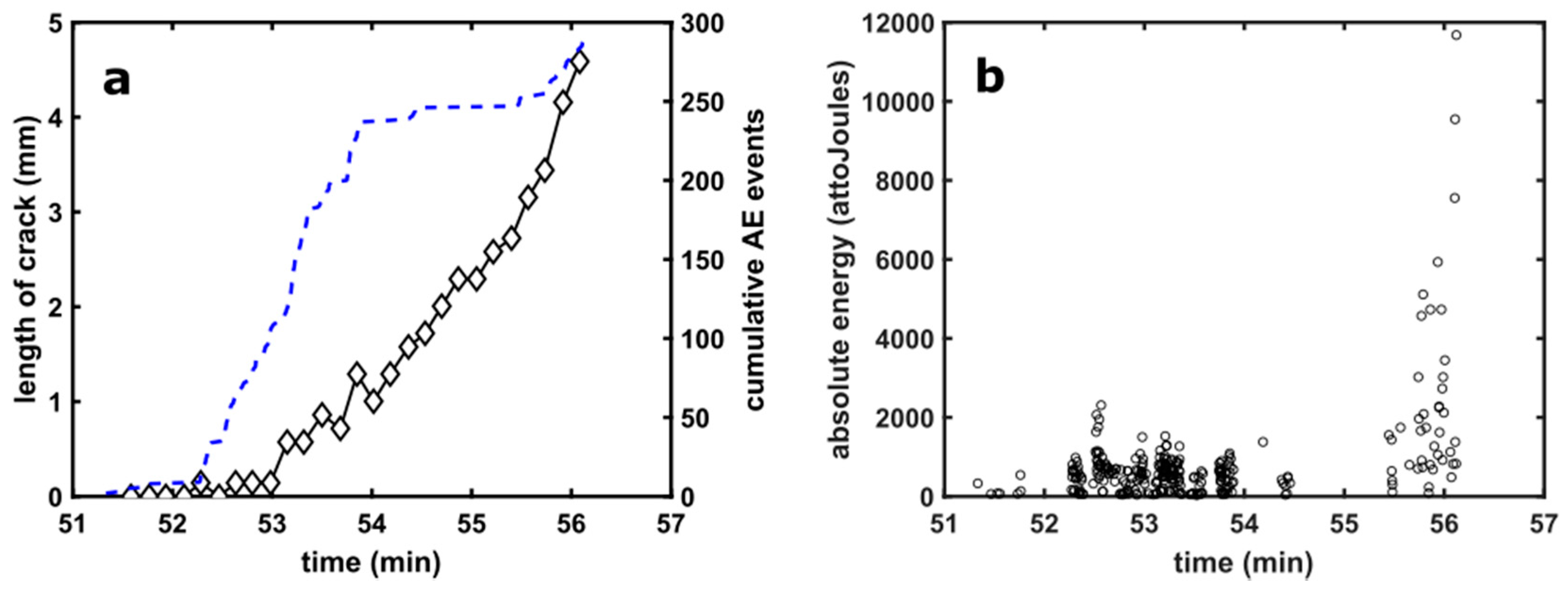
The first indications of cracking behaviour were detected in the AE data 51 min 20 s after fatigue cycling began. It can be seen in Figure 2a that AE events began to be recorded at this time, and that these were low energy events (Figure 2b). The optical flow technique indicates the initiation of a crack tens of seconds later. Both the number of AE events and the energy of each individual event show a general increase until 56 min, when full failure of the specimen occurred. The crack length, as calculated from the optical flow algorithm, also increases to a length of 4.6 mm in the same timeframe (Figure 2a). Just before final failure, there is a large increase in the energy released during each AE event, which would be expected as crack propagation speed increases during failure of the specimen.

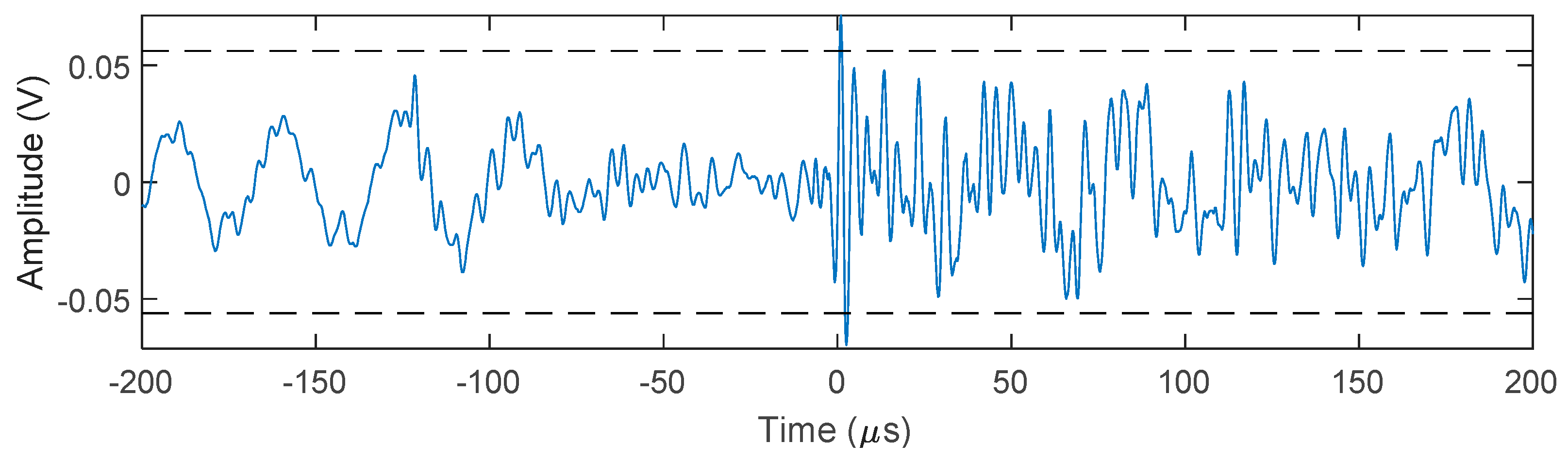
A plateau in the AE events can be seen between approximately 54 min and 55 min 30 s; however, the same trend is not seen in the crack length as measured by TSA. This apparent reduction in AE activity is unexpected, as the crack growth activity is expected to continue throughout, producing AE events. Examination of events before and after this plateau reveals that the amplitudes are only just above the 55 db threshold, therefore we assume that events were “just missed” due to the high threshold selected to eliminate background noise; this is exemplified in Figure 3 which shows a typical AE hit from this experiment. This hit was recorded on AE channel 1 as part of an event calculated to have originated from the region of cracking (corresponding to x = −5.89 cm and y = −1.24 cm in Figure 4). It can be seen that the constant background noise, clearly visible in the pre-trigger region (before time = 0), is relatively high, reaching 0.0458 V, or 52.22 dB, in this particular example, with the vast majority of its energy at 30 kHz. The transient energy arriving at the trigger point is characteristic of AE originating from crack growth activity due to its high rise time and frequency content [20], with the majority of the energy in this instance contained between 200 and 330 kHz likely owing to the resonance of the sensors in this region.

It is possible to consider using both the TSA and AE data here to determine criteria for damage detection, and to indicate that a crack has reached a critical length. If data analysis is carried out in real-time, these criteria could be used to indicate that a test should be stopped, or a part repaired or replaced in an engineering structure. This may be easier with the optical flow algorithm, as a crack length is reported, so a critical length could be defined at which the test ends or a component is replaced or repaired. It would also be possible to calculate the growth rate of the crack and identify a critical propagation rate. A similar approach could be taken for the AE data, either by determining a critical number of events reported, or an energy threshold for those events.

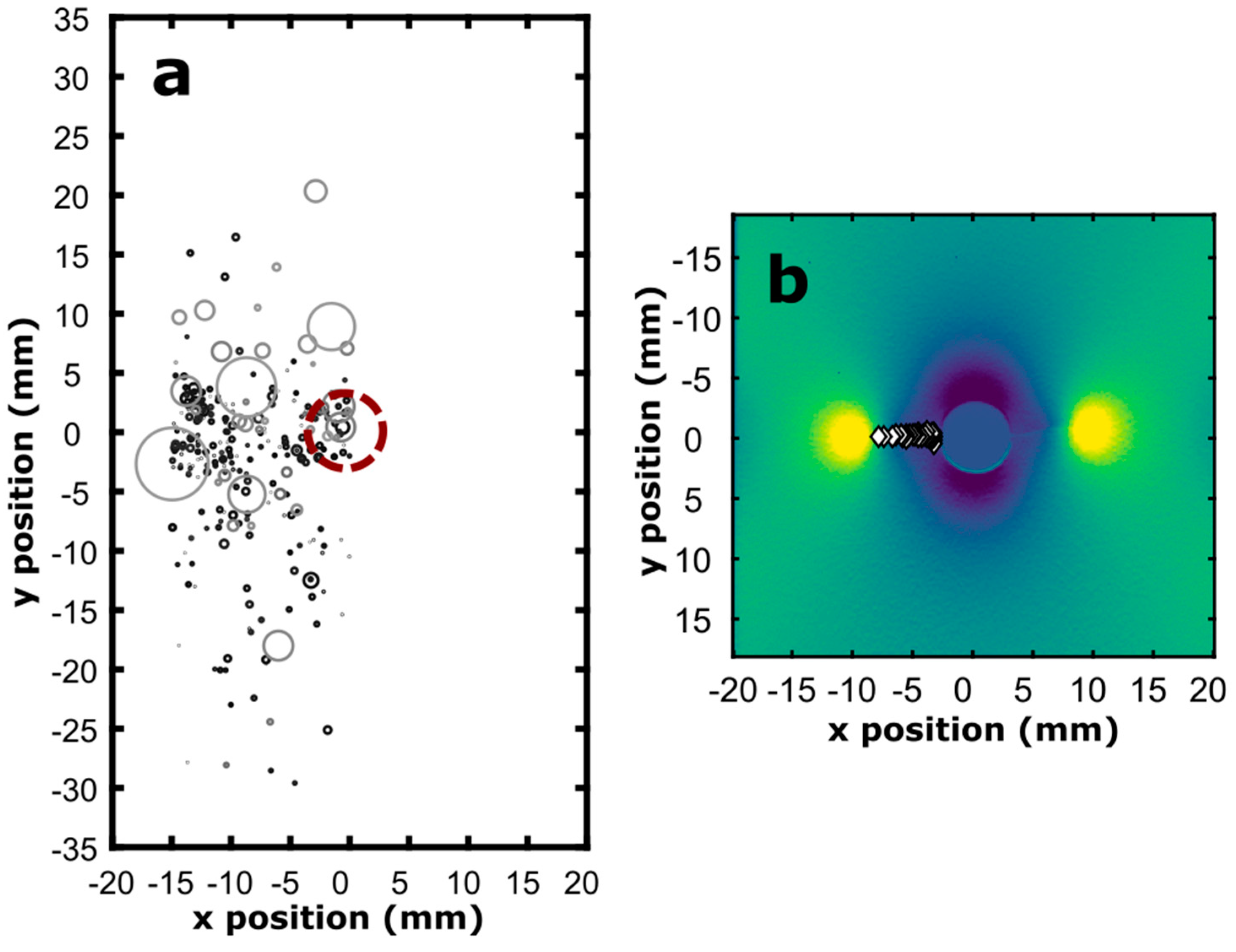
The position of identified AE events located with Delta-T Mapping can be seen in Figure 4a, where most events are clustered around the crack position. However, events were also registered far from the crack, at up to 30 mm from the crack path. As seen in Figure 2b, the later events are higher energy but there is no correlation between time and expected crack-tip position (i.e., later, larger energy events are not closer to the edge of the specimen). Though unmeasurable, as the true source locations are unknown, it would appear that the error in the location of AE signals collected during the experiment is larger than the 1.71 mm error calculated in the preliminary location study (for example, locating events in the central hole). This is likely due to the fact that the preliminary location study was conducted with Hsu-Neilson sources, which give a large amplitude signal that are inherently easier to locate than the low amplitude signals recorded during this experiment. Furthermore, as the specimen was not being loaded in the test machine during the collection of preliminary data for the location study, it was not subject to the noise which is present in the experimental data. The structured noise in the experimental data likely acts to reduce the accuracy of the identification of the start time of the hit using the Akaike Information Criterion which forms part of the Delta-T Mapping process (for a full description, see [15]), thus giving a lower accuracy of location than expected.

In contrast, the crack-tip positions located with the optical flow analysis of TSA data are shown in Figure 4b. The optical flow data have been reflected about the longitudinal axis to allow direct comparison with the AE data, and only data from the left-hand side of the hole are shown for both TSA and AE results, as this was the first crack to initiate. The optical flow results are much closer to the crack path than the AE events, and have previously been shown to match well with the final crack morphology [9].

It should be noted that the specimen geometry was chosen based on previous TSA experiments [9]. Therefore, it was designed to produce optimum conditions for the TSA method to locate the crack position, but not the AE. In fact, the small size of the specimen means that the AE sensors are positioned very close to one another, meaning that the difference in time of arrival of signals between one sensor and another is also small, and thus the inherent recording errors have a very large impact on the accuracy of the technique in this instance. Furthermore, the size of the specimen creates a situation where there will be multiple large amplitude reflected signals which will also produce erroneous locations. This said, for practical SHM purposes the ability to detect a cluster of high energy events to within 30mm of a source of damage may be adequate information for maintenance purposes.

Evidently, in real world applications, the situation is extremely unlikely to be ideal for any technique. When using NDT techniques to locate damage in engineering structures, it is therefore important to consider what information is most important, and the constraints on the testing, for example, whether access is available for contact techniques. Here, with a simple specimen geometry, it is possible to say that TSA results in more accurate detection of the crack-tip position, but AE results in an earlier indication of damage.

All raw TSA and AE data discussed in this paper is available as supplementary information, deposited in the University of Liverpool Data Catalogue.

4. Conclusions

Two non-destructive testing methods have been applied during fatigue crack initiation and propagation in a metallic specimen during tension–tension cyclic loading. Thermoelastic stress analysis and acoustic emission data were collected and a comparison of processed data shows that AE can indicate the presence of damage slightly earlier in time, whereas optical flow analysis of TSA data can generate more precise location information. These results show that the aim of the testing should be considered before deciding on an appropriate NDT method, and that the use of a combination of methods may yield more information than only one.

References

- Sakagami, T. Remote nondestructive evaluation technique using infrared thermography for fatigue cracks in steel bridges. Fatigue Fract. Eng. Mater. Struct. 2015, 38, 755–779. [Google Scholar] [CrossRef]
- Sharpe, W.N. Springer Handbook of Experimental Solid Mechanics; Springer: Berlin, Germany, 2008; ISBN 978-0-387-26883-5. [Google Scholar]
- Lemaitre, J.; Dufailly, J. Damage measurements. Eng. Fract. Mech. 1987, 28, 643–661. [Google Scholar] [CrossRef]
- Greene, R.J.; Patterson, E.A.; Rowlands, R.E. Thermoelastic stress analysis. In Springer Handbook of Experimental Solid Mechanics; Sharpe, W.N., Ed.; Springer: Berlin, Germany, 2008; pp. 743–767. ISBN 978-0-387-26883-5. [Google Scholar]
- Dulieu-Barton, J.M. Introduction to thermoelastic stress analysis. Strain 1999, 35, 35–39. [Google Scholar] [CrossRef]
- Diaz, F.A.; Patterson, E.A.; Tomlinson, R.A.; Yates, J.R. Measuring stress intensity factors during fatigue crack growth using thermoelasticity. Fatigue Fract. Eng. Mater. Struct. 2004, 27, 571–583. [Google Scholar] [CrossRef]
- Ancona, F.; Palumbo, D.; De Finis, R.; Demelio, G.P.; Galietti, U. Automatic procedure for evaluating the Paris Law of martensitic and austenitic stainless steels by means of thermal methods. Eng. Fract. Mech. 2016, 163, 206–219. [Google Scholar] [CrossRef]
- Rajic, N.; Brooks, C. Automated Crack Detection and Crack Growth Rate Measurement Using Thermoelasticity. Procedia Eng. 2017, 188, 463–470. [Google Scholar] [CrossRef]
- Middleton, C.A.; Gaio, A.; Patterson, E.A.; Greene, R.J. Towards Automated Tracking of Initiation and Propagation of Cracks in Aluminium Alloy Coupons Using Thermoelastic Stress Analysis. J. Nondestruct. Eval. 2019, 123. [Google Scholar] [CrossRef]
- Rajic, N.; Street, N.; Brooks, C.; Galea, S. Full field stress measurement for in situ structural health monitoring of airframe components and repairs. In Proceedings of the 7th European Workshop on Structural Health Monitoring, Nantes, Frances, 8–11 July 2014. [Google Scholar]
- ASTM Standard E610. Standard Terminology Relating To Acoustic Emission; ASTM International: West Conshohocken, PA, USA, 1989. [Google Scholar]
- Miller, R.K.; Findlay, R.D.; Carlos, M.F. Acoustic Emission Testing. In NDT Handbook; American Society for Nondestructive Testing: Columbus, OH, USA, 2005; pp. 122–146. [Google Scholar]
- Baxter, M. Damage Assessment by Acoustic Emission (AE) During Landing Gear Fatigue Testing; Cardiff University: Cardiff, UK, 2007. [Google Scholar]
- Eaton, M.J.; Pullin, R.; Holford, K.M. Acoustic emission source location in composite materials using Delta T Mapping. Compos. Part A Appl. Sci. Manuf. 2012, 43, 856–863. [Google Scholar] [CrossRef]
- McCrory, J.P.; Pullin, R.; Pearson, M.R.; Eaton, M.J.; Featherston, C.; Holford, K.M. Effect of Delta-T Grid Resolution on Acoustic Emission Source Location in GLARE. In Proceedings of the 30th European Conference on Acoustic Emission Testing, Granada, Spain, 12–15 September 2012. [Google Scholar]
- Pearson, M. Development of Lightweight Structural Health Monitoring Systems for Aerospace Applications; Cardiff University: Cardiff, UK, 2013. [Google Scholar]
- ASTM. Standard Practice for Verifying Acoustic Emission Sensor Response, Active Standard ASTM F2174; ASTM International: West Conshohocken, PA, USA, 2015. [Google Scholar]
- Eaton, M. Acoustic Emission (AE) Monitoring of Buckling and Failure in Carbon Fibre Composite Structures; Cardiff University: Cardiff, UK, 2007. [Google Scholar]
- ASTM Standard E976. Standard Guide for Determining the Reproducibility of Acoustic Emission Sensor Response; ASTM International: West Conshohocken, PA, USA, 2015. [Google Scholar]
- Mazur, K.; Wisner, B.; Kontsos, A. Fatigue Damage Assessment Leveraging Nondestructive Evaluation Data. J. Met. 2018, 70, 1182–1189. [Google Scholar] [CrossRef]
© 2019 by the authors. Licensee MDPI, Basel, Switzerland. This article is an open access article distributed under the terms and conditions of the Creative Commons Attribution (CC BY) license (http://creativecommons.org/licenses/by/4.0/).