Case Depth Prediction of Nitrided Samples with Barkhausen Noise Measurement

Abstract

Nitriding is a heat treatment process that is commonly used to enhance the surface properties of ferrous components. Traditional quality control uses sacrificial pieces that are destructively evaluated. However, efficient production requires quality control where the case depths produced are non-destructively evaluated. In this study, four different low alloy steel materials were studied. Nitriding times for the samples were varied to produce varying case depths. Traditional Barkhausen noise and Barkhausen noise sweep measurements were carried out for non-destructive case depth evaluation. A prediction model between traditional Barkhausen noise measurements and diffusion layer hardness was identified. The diffusion layer hardness was predicted and sweep measurement data was used to predict case depths. Modelling was carried out for non-ground and ground samples with good results.

1. Introduction

Barkhausen noise (BN) measurement is a non-destructive testing method suitable for ferromagnetic materials, which can be used to aid in grinding burn detection and material characterisation. BN has been found to be sensitive to changes in many material properties, for example, a relationship has been observed between material hardness [1,2] and residual stress state [2,3]. The main challenges in the evaluation of material properties from BN measurement signals are the complex interactions between material properties and BN due to the stochastic nature of BN and the case-dependency of the evaluation models. In addition, changes in material properties accumulate to the BN measurement signal making it difficult to distinguish between individual effects. The Barkhausen noise signal as such is quite useless, but some features can instead be computed and then compared with the material properties of interest. Traditional features are the root-mean-square value (RMS) and the height, width, and position of the so-called BN profile. Many other features can also be used but they are not listed here. Instead, an interested reader can find these in [4]. Based on the features computed, the interactions between BN and the material properties can be evaluated. If the aim is to predict some material property from the measured BN signal, the features computed are used as input variables in the prediction model.

Some studies were identified in the literature that modelled material properties and BN. In [2] and [5] for example, linear models were identified for mapping the interactions between BN, and residual stress and hardness. Use of nonlinear model structures can also be found in the literature. For example, it was found in [6] that a second order polynomial is suitable for mapping the relationship between the properties of dual-phase steel and BN. Another study [7] suggested that nonlinear model structures should be used for the prediction of residual stress based on the BN measurement. Nonlinear black-box modelling techniques have also been used. Backpropagation neural networks were used in [8] to predict the stress applied to A3 type steel. In [9], an adaptive neuro-fuzzy system (ANFIS) was used to evaluate the microstructure of dual-phase steel. The drawback of black-box methods is that their identification may be challenging, and the risk of overfitting is evident because BN data sets usually have a limited number of data points. Another problem in modelling is the uncertainty of the BN measurement and the variation caused by the material properties that are not measured. These challenges combined often produce data sets where the source of a significant part of the variation cannot be identified, which makes the use of more complex model structures less intriguing.

A so-called BN sweep measurement can be used in the evaluation of case depth for nitrided samples [10]. The measurement is based on the voltage sweep carried out prior to the actual BN measurement to determine a suitable magnetisation voltage. Figure 1 shows an example of a voltage sweep. In a prior study [10], it was found that the sweep holds information relevant for evaluating case depth. That information can be revealed by finding the maximum slope of the sweep and the corresponding voltage (slope position), as shown in Figure 1. When these values are determined from sweeps carried out with low (20 Hz) and high (125 Hz) magnetisation frequencies, the ratio of slopes has a linear relationship with case depth [10]. The slope positions have also been noticed to hold information about the residual stress state of the material [11]. Even though a linear relationship was observed in [10], the authors also noticed that the relationship depended on surface hardness.

Only a few studies have been published regarding nitrided samples and the traditional relation of the Barkhausen noise signal. Case depths of ion nitrided steel samples, with case depths varying from 1 to 200 µm, were studied in [12]. They noticed a linear relationship between case depth and the BN values that were evaluated based on a certain frequency range [12]. A frequency range analysis was also carried out by the authors of [13] who studied nitrided, ground, and differently shot peened samples manufactured from 32CD4 steel. They established a correlation between results from BN measurements and residual stress depth distributions obtained using X-ray diffraction. The frequency analysis was carried out to obtain information at certain depths in the samples [13]. The response of the BN signal to grinding damage in nitrided steels was studied in [14]. The authors noticed that the sensitivity to small changes in the microstructure was much stronger than the sensitivity to the level of residual stress in the nitrided carbon steel samples.

Rolled and nitrided steel sheet C10 samples were studied with Barkhausen noise and X-ray diffraction in [15], the authors utilised magnetising voltage sweep measurements and noticed different behaviour of the voltage sweep outcomes between two samples with different compound layer thicknesses. The compound layer thickness also had an influence on the traditional RMS value. In addition, another study [16] utilised the magnetising sweep measurement method for inspecting different compound layer thicknesses on three different nitrocarburised samples as a method of verifying the heat treatment process. A good correlation was found between the magnetising voltage sweep, and the compound layer and diffusion layer thickness with all the steels studied. In addition, the BN full width at half maximum (FWHM) was found to correlate with the compound and diffusion layer thicknesses. The compound layer was electropolished, and the measurements were repeated. The polished samples that had the compound layer taken off showed an even stronger correlation between the magnetizing voltage sweep and the nitrided layer thickness [16].

In this study, the use of magnetizing voltage sweep measurements in case depth evaluation is further studied. Two schemes are considered in which BN measurements are carried out on non-ground and ground surfaces. The compound layer on non-ground surfaces does not significantly contribute to the Barkhausen noise measurement [17], and thus it is expected that the correlation between case depth and Barkhausen noise will deteriorate. In this paper, a specific point of interest is if the effect of diffusion layer hardness can be eliminated. A two-step modelling scheme was applied. In the first step, the diffusion layer hardness of the samples was evaluated based on traditional BN features. In the second step, another regression model was identified for the evaluation of case depth, where the predicted hardness and the slope ratio were used as input variables. Both models used a multiple linear regression model including the main and interaction terms. The modelling was carried out for the data set obtained from a set of nitrided samples.

2. Materials and Methods

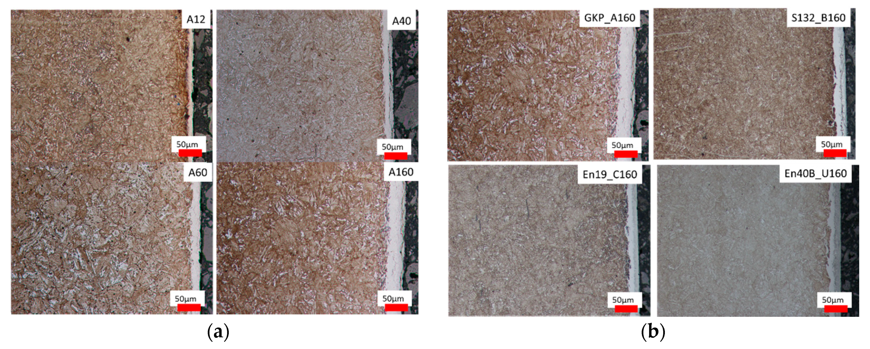
2.1. Material Description

The sample set used in the study consisted of 16 flat samples with dimensions of 12 mm × 10 mm × 170 mm. The samples used in the study were fabricated from the materials shown in

Table 1. Materials used.

Series Name	Material	Samples *	Threshold Values for Case Depth (HV)
A	GKP	A12, A40, A80, A160	550
B	S132	B12, B40, B80, B160	520
C	En19	C12, C40, C80, C160	400
U	En40B	U12, U40, U80, U160	400

* 12 = 12 h, 40 = 40 h, 80 = 80 h, and 160 = 2 × 80 h of nitriding.

, the chemical compositions of which are shown in

Table 2. Compositions of the materials [19].

Material	C (wt%)	Cr (wt%)	Mo (wt%)	V (wt%)	Mn (wt%)	Si (wt%)	P (wt%)	S (wt%)
GKP (32CrMoV5)	0.3	1.4	1.2	0.3
BS132	0.35–0.43	3.0–3.5	0.8–1.2	0.15–0.25	0.4–0.7	0.1–0.35	0.02	0.02
En19 (709M40)	0.36–0.44	0.9–1.2	0.25–0.35		0.7–1.0	0.1–0.35	0.035	0.04
En40B (722M24)	0.2–0.28	3.0–3.5	0.45–0.65		0.45–0.7	0.1–0.35	0.035–0.04

. Four different carbon steels were studied: 32CrMoV5 (GKP), BS S132 (S132), 709M40 (En19), and 722M24 (En40B) which were later named A, B, C, and U series, respectively. Four samples were prepared from each steel material with varying case depths. The samples were gas nitrided in a furnace for different times (12, 40, 80, or 160 h) to generate different case depths. Nitriding is a surface hardening method for alloy steels that employs a diffusion-based technique to modify the surface structure chemically [18]. During nitriding, the samples were heated in a furnace at 500–520 °C with ammonia gas with a 25–35% dissociation rate. The ammonia gas decomposes into hydrogen and nitrogen. Nitrogen is further soluted to ferrite to form different compounds. Two layers form during the nitriding, a compound layer (CL) and a diffusion layer (DF). The outer compound layer, which is referred to as the white layer, has a thickness of 5–30 µm and is composed of γ’ (Fe₄N) and ε (Fe₃N) nitrides [16]. This layer is hard, brittle, and is often removed by grinding. The variation in the case depth produced with constant nitriding parameters for different steel materials is due to the differences in chemical composition between the steel grades. Figure 2 presents the optical micrographs from the GKP samples (left) and samples GKP, S132, En19, and En40B with a constant nitriding time of 160 h (right).

2.2. Sample Preparation

The case depths for the different samples are given in

Table 3. Case depths (mm) of the studied samples.

Nitriding Time (h)	A (GKP)	B (S132)	C (En19)	U (En40B)
12	0.34	0.18	0.09	0.15
40	0.38	0.29	0.15	0.25
80	0.52	0.44	0.24	0.35
160	0.84	0.56	0.24	0.45

. The case depths were determined based on the ISO 6336 standard [20] via the measurement of micro-hardness profiles. The material-dependent threshold values given in Table 1 were used to obtain the case depths. An example of case depth profiles and case depth determination is given in Figure 3. After nitriding, a compound layer—also referred to as the white layer—was present on the surface of the samples. The first measurements were carried out with the compound layer still on the samples, while the second set of measurements were carried out with the compound layer ground off. The grinding was carried out using a Jones and Shipman 540 hydraulic surface grinder (Jones and Shipman, Rugby, UK) fitted with an aluminium oxide grinding wheel. The wheel speed was 3000 rpm (28 m/s), the infeed was 0.01 mm, and the feed rate was approximately 15 m/min. In each case, the grinding depth was based on the measured white layer thickness. Five measurement locations were fixed for each sample. The locations were 25, 50, 75, 100, and 125 mm from the edge of the sample.

2.3. Measurement Devices

The BN measurements were carried out with a Rollscan 300 measurement device manufactured by Stresstech Oy (Vaajakoski, Finland). The magnetising frequency and voltage used were 125 Hz and 10 V_pp (voltage peak to peak). The sampling frequency was 2.5 MHz. The BN measurement signals were stored, and the BN features were computed using Stresstech MicroScan software (Stresstech Oy, 6.0.0r1596, Vaajakoski, Finland). The BN measurements were carried out in the longitudinal direction of the samples and the raw measurement signals were filtered to the 70–200 kHz frequency band.

The BN sweep measurements were also carried out with the Rollscan 300 device (Stresstech Oy, Vaajakoski, Finland) using Stresstech PCCaseDepth software for computing. The magnetising voltage was increased with 0.1 V_pp increments from 0 to 16 V_pp. The sweeps were recorded with magnetising frequencies of 20 and 125 Hz. Surface hardness values were measured with Matsuzawa NMT-X7 (Matsuzawa Co. LTD, Akita, Japan) hardness tester with the applied load for these Vickers hardness measurements of 1 kg. Hardness depth profiles were measured using a Buehler MMT-7 micro-hardness tester (Buehler, Lake Bluff, IL, USA) with a load of 300 g. The optical micrographs were taken with Nikon DS-L2 optical microscope (Nikon, Tokio, Japan).

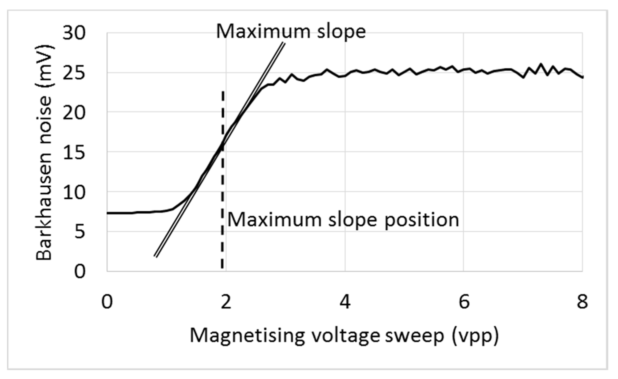
2.4. Measurements and Data Pre-Processing

The sweep measurements were processed so that the slope and slope position values were obtained. A detailed description of the computations needed for obtaining these features is given in [10]. The traditional features computed are the RMS value, peak width, and peak position. Peak height is not used here because it is reported to have a great correlation with the RMS value [5] and thus does not provide any additional information for the model. The sweep measurements were taken from five locations on each sample. The results from these five repetitions were averaged so that one value was obtained for each sample. It was observed that the measured data set contained outliers and thus averaging was carried out in two steps. First, the minimum and maximum values were removed, then the average of the remaining three values was taken. Thus, it was assumed that the obtained values represented the samples well. Diffusion layer hardness values for modelling were taken from a depth of 0.05 mm from sample surface.

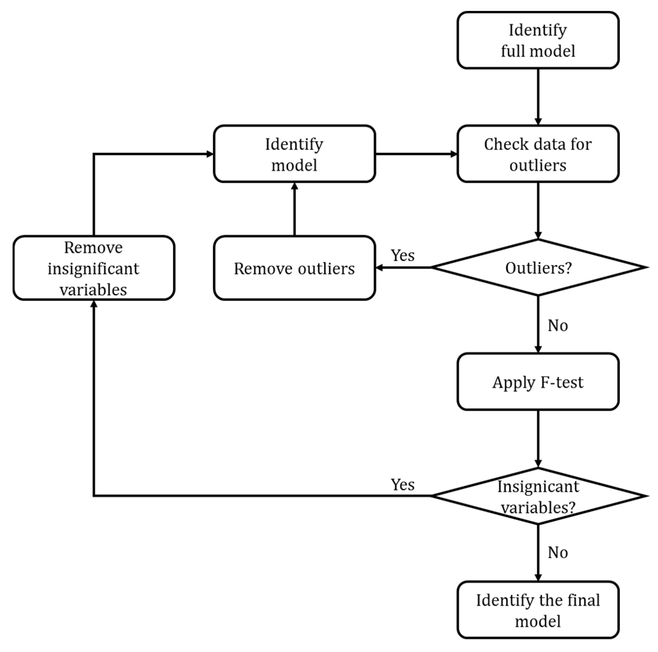
2.5. Modelling Approach

It was observed in [10] that the ratio of the slopes obtained from 20 and 125 Hz sweep measurements had a linear relationship with case depth. However, it was also noticed that surface hardness had an effect on the relationship. Thus, this study aimed to compensate the effect of diffusion layer hardness by including it in the model that was used for case depth evaluation. The modelling scheme was divided into two steps. First, the diffusion layer hardness was evaluated with the traditional BN features, this predicted hardness was then used as an input variable together with the slope ratio in an attempt to evaluate the case depths of the samples.

A multiple linear regression (MLR) model with single variable and two variable interaction terms was used in this study. The identification of both the aforementioned models included the following steps:

• Identification of the full model (all features and their two-variable interactions);
• Detection of outliers;
• Elimination of excess terms from the model;
• Identification of the model with the appropriate terms excluding the detected outliers;
• Evaluation of the model performance and structure.

These steps were repeated as long as insignificant terms or outliers were found. As a final validation step, the standard error of regression coefficients was checked. Figure 4 illustrates the model identification scheme applied. Elimination of insignificant terms was carried out by calculating the ANOVA table for the model and then applying an F-test for the terms. Together with the F-test criterion, the p-value was also computed. The p-value is the risk of the wrong result when the term is declared significant. A risk level of 0.05 was used in this study. Thus, if the p-value was greater than 0.05 the term was declared insignificant. The suitability of the model structure was evaluated based on a normal probability plot of the residuals. Outliers were evaluated from the residuals. If a residual got a large value, the corresponding data point was considered an outlier. The final model—with insignificant terms and outliers excluded—was evaluated with an R-squared value, the root mean squared error of prediction (RMSE), the normal probability plot of residuals, and visually from a scatter plot of measured vs. predicted case depth values. The significance of individual terms in the models were evaluated based on their relative contribution to the model output. The relative contribution was obtained by calculating the change of model output when individual terms varied 10% around their average values. This sensitivity was divided by the overall sensitivity to obtain the contribution of each term. The direction of contributions can be seen from the sign of the estimated regression coefficient value.

3. Results

Modelling was carried out for the data sets obtained with and without the compound layer present. The models were identified through the procedure described in Section 2.5. Here, the results of the modelling steps are given together with their discussion.

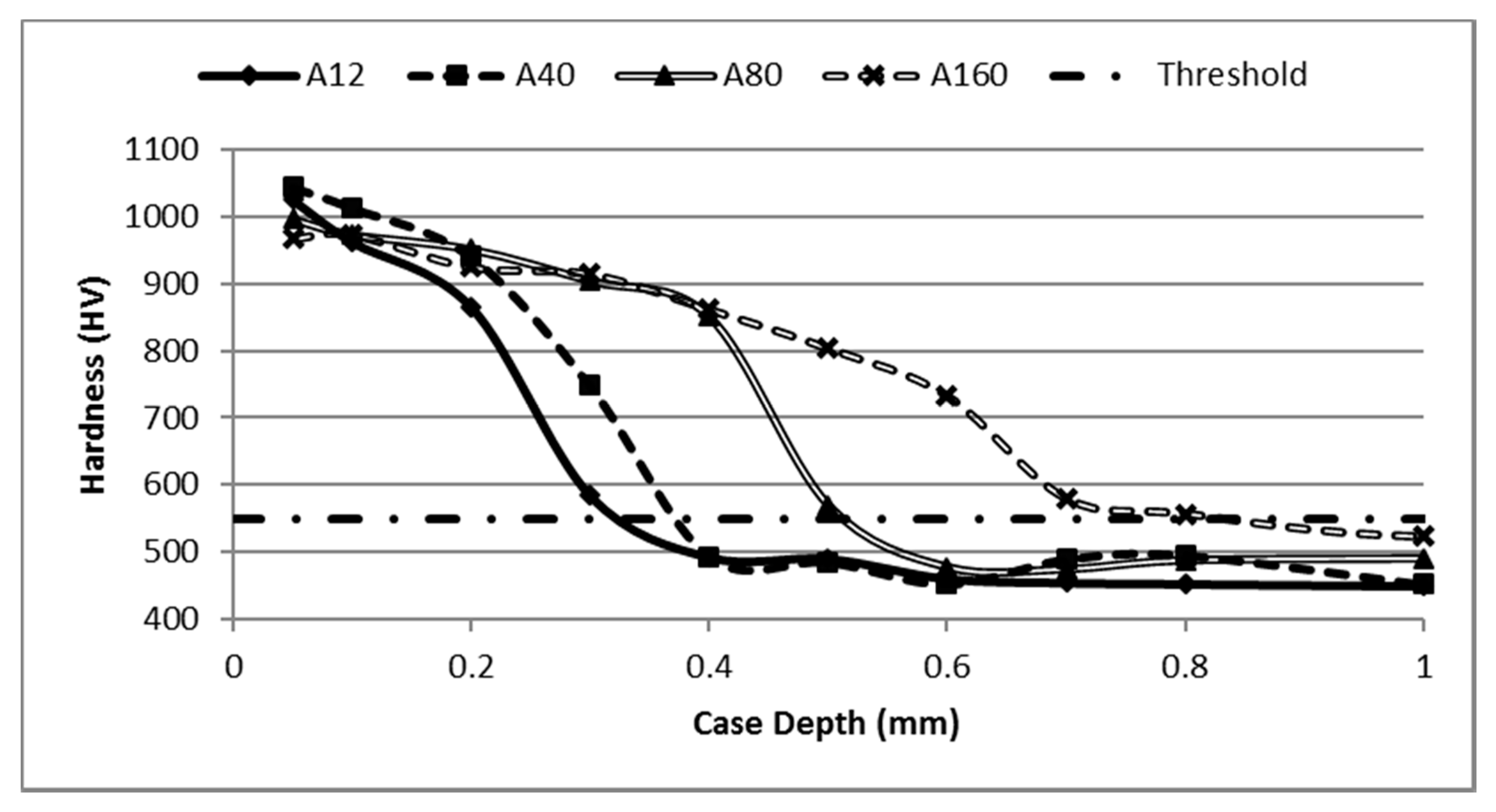
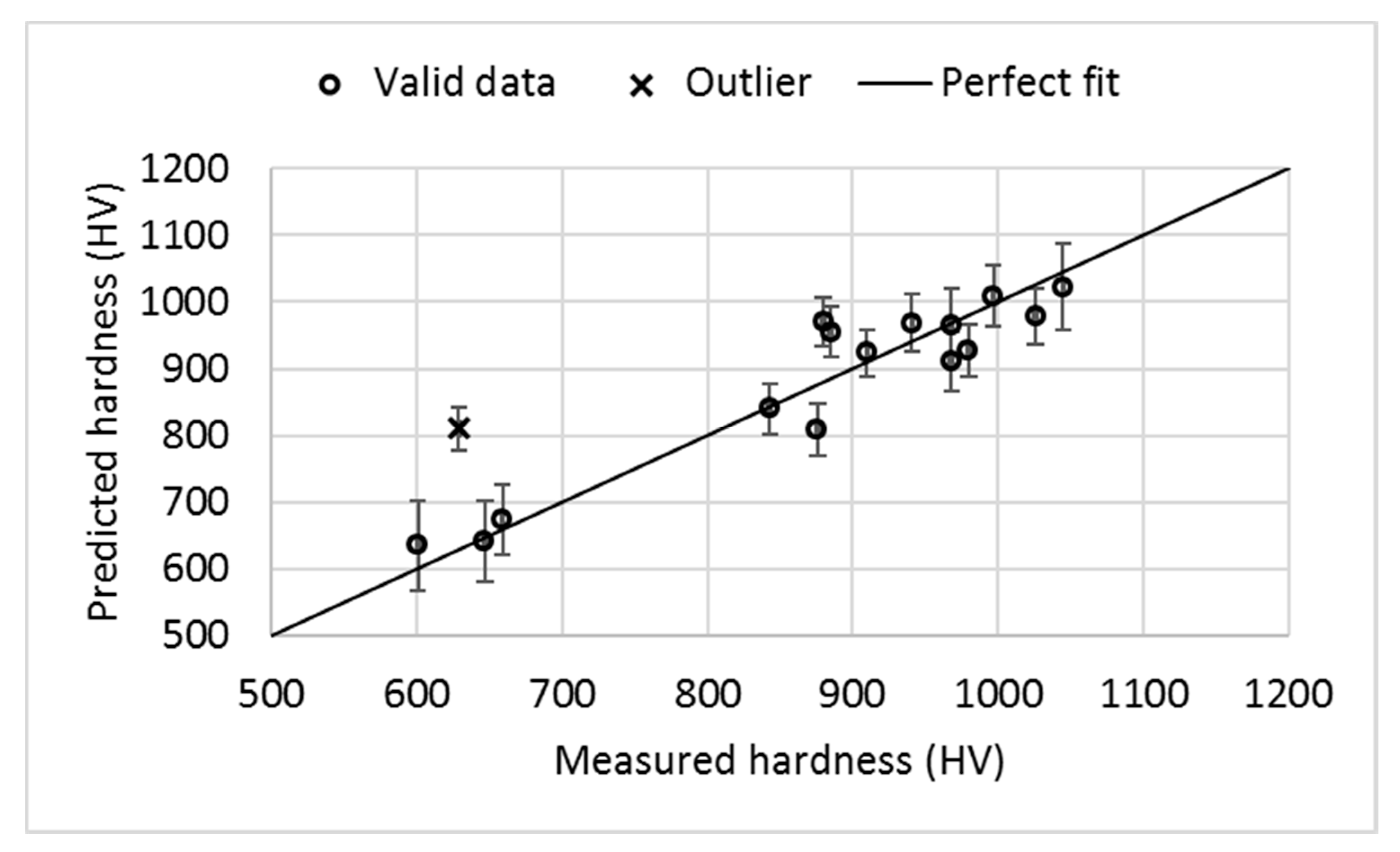
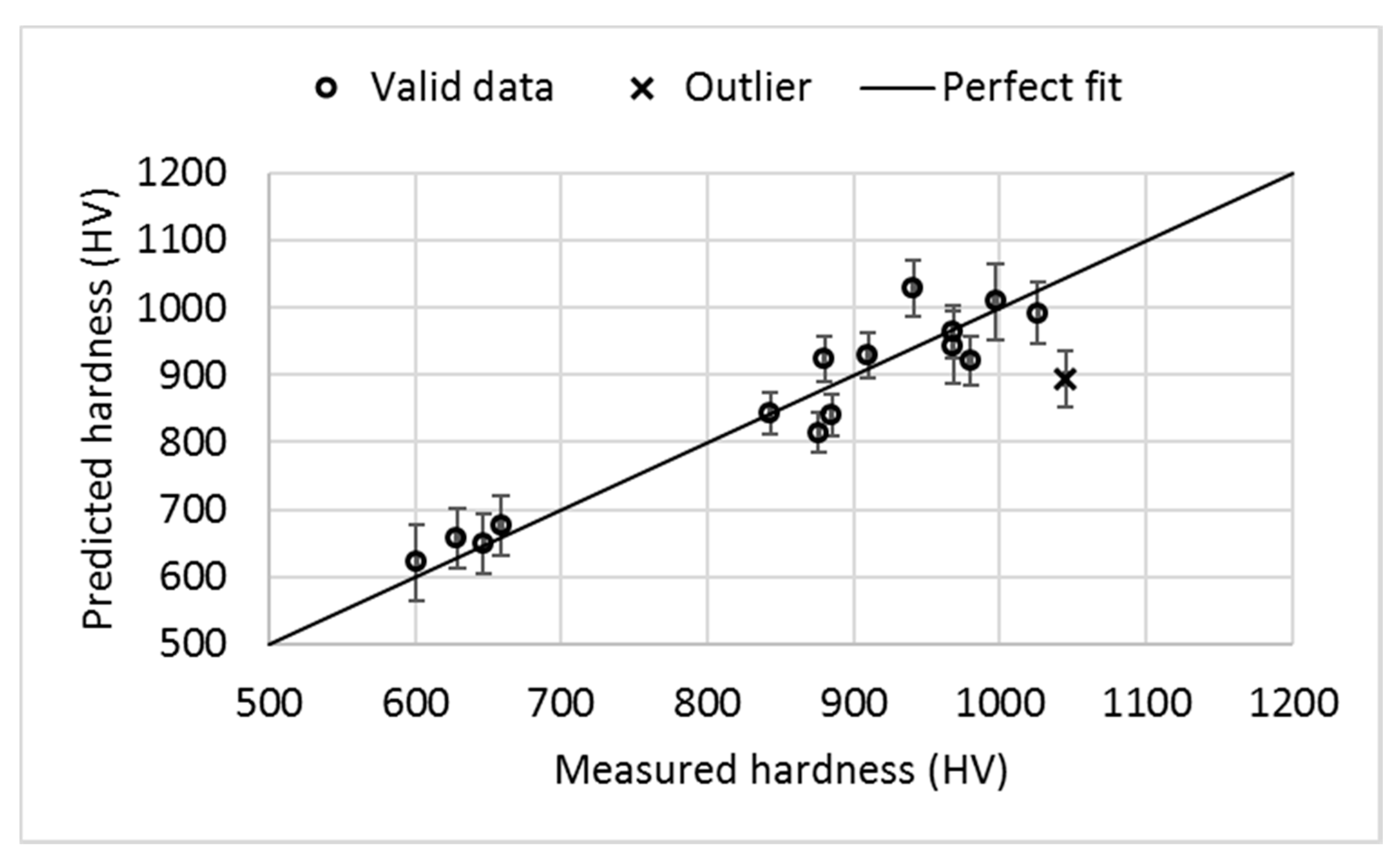
3.1. Modelling of Hardness

As mentioned above, surface hardness is evaluated based on traditional BN features, these are the RMS value, peak width, and peak position. The full model that is first identified is given by the equation:

$$y_{HV}=a_0+a_1{x}_{rms}+a_2{x}_p+a_3{x}_w+a_{12}{x}_{rms}{x}_p+a_{13}{x}_{rms}{x}_w+a_{23}{x}_p{x}_w.$$

(1)

where y_HV is hardness, x_rms is the RMS value, x_p is the peak position, x_w is the peak width, and a_ij are the regression coefficients. This model was then subjected to a possible elimination of insignificant terms and outliers. The following subsections give the results for the data sets of non-ground and ground samples.

3.1.1. Non-Ground Samples with Compound Layer

The full model was identified first. The residuals of the full model were computed, and one outlier was detected. This outlying point was removed, and the model was identified again. The F-tests applied indicated that all the terms with peak width (x_w, x_rmsx_w, and x_px_w) are to be removed from the model. It was further noticed that the standard error of peak position was very high compared with the regression coefficient and thus that term was also removed. No more outliers or insignificant terms were found, and thus the final model excluding the insignificant terms and the outlying data point was identified.

Table 4. The regression coefficients, standard errors, p-values, and contributions for the model of hardness with the non-ground sample data set. The intercept term is a₀ = 646.52.

Term	Coefficient	Standard Error	p-Value	Contribution (%)
xrms	a1 = −6.70	0.76	1.28 × 10−6	45.5
xrmsxp	a12 = 0.54	0.054	3.35 × 10−7	54.5

shows the values of the regression coefficients together with their standard errors, p-values, and contributions for the model. The standard errors are low compared with the coefficient values and contributions are significant. The R² value of the model is 0.90 and the RMSE value is 49.0 HV. Figure 5 shows the predicted hardness as a function of the measured hardness. The model performance indices in Figure 5 indicate that the prediction model for hardness with the data set of non-ground samples is valid.

3.1.2. Ground Samples

The results obtained with the ground sample data set are very similar to those obtained with the non-ground data set. The same terms were eliminated from the model, and one outlier was detected. The R² value of the obtained model is 0.92 and the RMSE value is 43.7 HV.

Table 5. The regression coefficients, standard errors, p-values, and contributions for the model of hardness with the ground sample data set. The intercept term is a₀ = 685.83.

Term	Coefficient	Standard Error	p-Value	Contribution (%)
xrms	a1 = −5.14	0.50	2.47 × 10−7	41.4
xrmsxp	a12 = 0.42	0.036	6.27 × 10−8	58.6

gives the values of the regression coefficients together with their standard errors, p-values, and contributions. Figure 6 shows the graph of predicted vs. measured hardness. Low standard errors and significant contributions shown in Table 5 indicate that the terms in the model are valid.

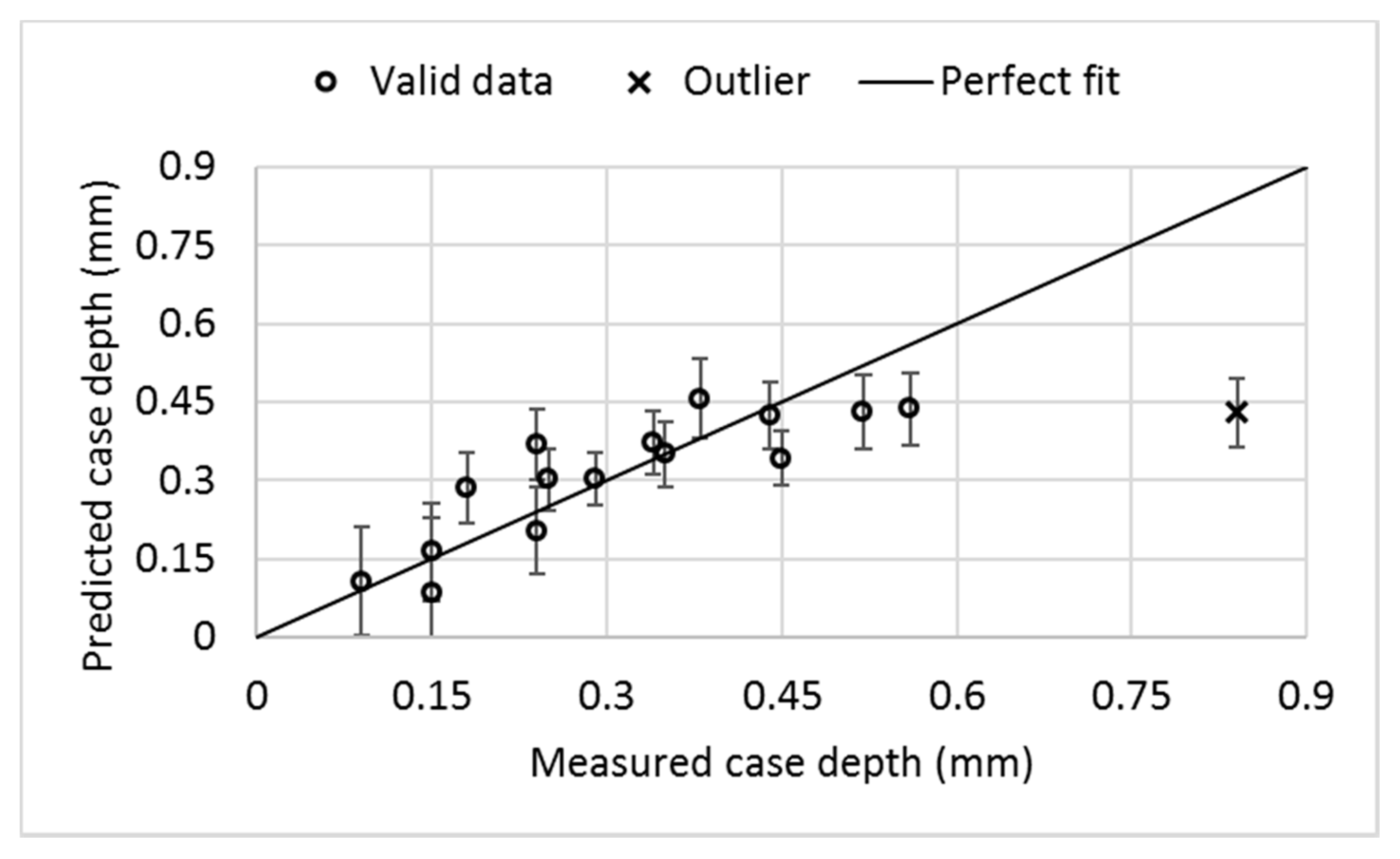
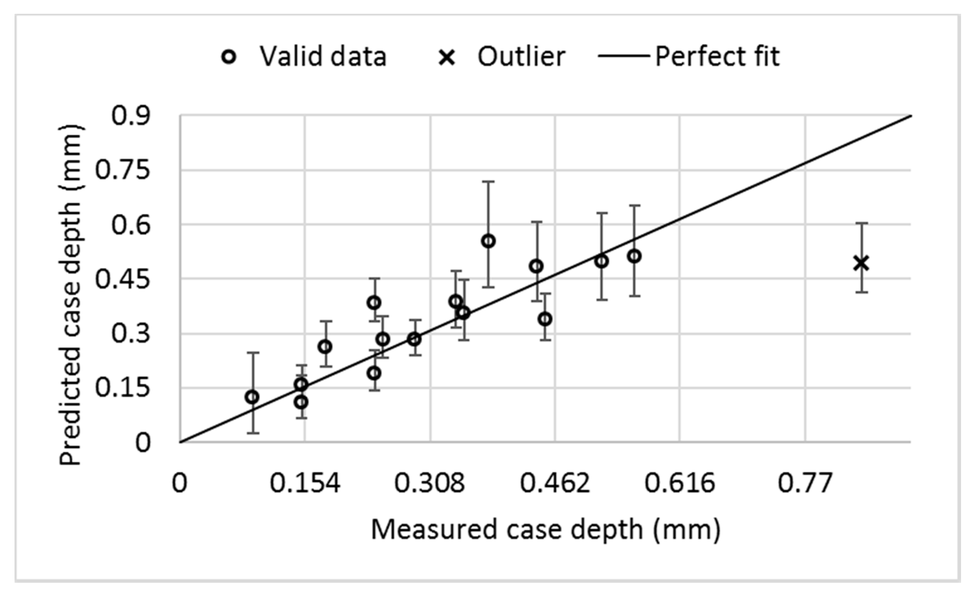
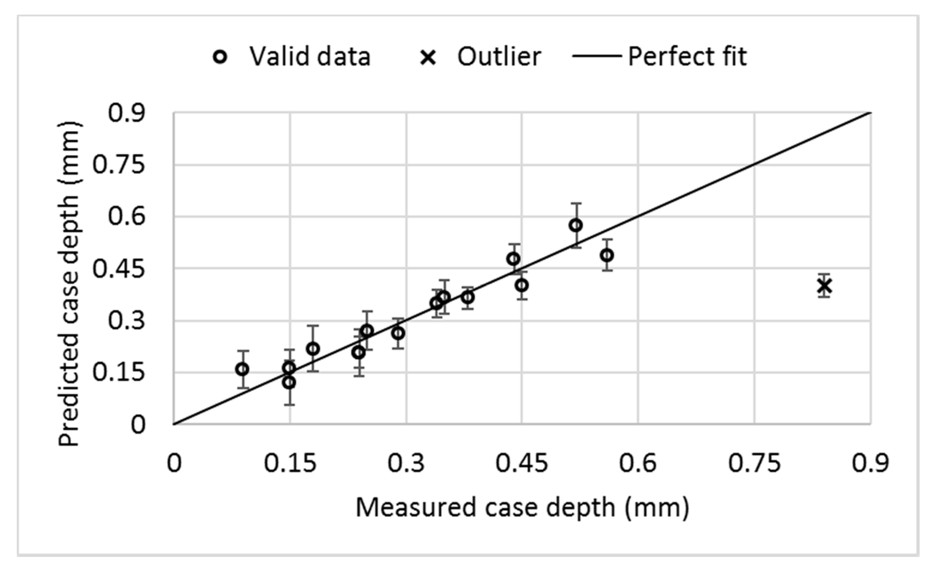
3.2. Modelling of Case Depths

The input variables for the model of case depth are the predicted hardness and slope division. There are two options for how to compute the slope division. In the original paper [10], the slope of the 20 Hz sweep was divided by the slope of the 125 Hz sweep but vice versa is also possible. In this paper, both options were tested but only one of them was included in the model. The full model for case depth evaluation is:

$$y_{CD}=b_0+b_1{x}_{HV}+b_2{x}_{SD}+b_{12}{x}_{HV}{x}_{CD}.$$

(2)

where y_CD is the case depth, x_SD is the slope division, and b_ij are the regression coefficients. Again, this model is subjected to elimination of insignificant terms and outliers.

3.2.1. Non-Ground Samples with Compound Layer

First, both options for slope division were tested. For the non-ground data set, division of the 20 Hz slope with the 125 Hz slope was more beneficial and thus that was used in the model. The full model was then identified. The residuals showed one outlying data point, which was removed, then the model was identified again. The F-tests suggested that the two variable interaction term should be removed from the model. No more outliers or insignificant terms were found and thus the final model was identified excluding the outlier and the interaction term. The regression coefficients, their standard errors, p-values, and contributions are given in

Table 6. The regression coefficients, standard errors, p-values, and contributions for the model of case depth with the non-ground sample data set. The intercept term is b₀ = −0.51.

Term	Coefficient	Standard Error	p-Value	Contribution (%)
xHV	b1 = 0.0012	0.00022	0.00015	49.4
xSD	b2 = −0.54	0.12	0.00068	50.6

and the predicted vs. measured case depth is shown in Figure 7. Both terms have a high contribution to model output and standard errors are low. The model performance indices are: R² = 0.72; and RMSE = 0.081 mm. The R² value indicated that the model was reasonable but not as good as the hardness models presented in Section 3.1. Figure 7 shows that the correlation between predicted and measured case depth is not linear but the predictions show saturating behaviour. This indicates that the model structure may not be valid. Thus, another model was identified. This time the variable that was predicted was the logarithm of case depth.

A series of mathematical conversions for case depth were tested to compensate for the saturating behaviour in Figure 7. The conversions tested were the reciprocal, logarithm, exponential, and negative exponential. Among these, logarithm seemed to best compensate the saturating behaviour. The model for the logarithm of case depth was identified similarly to the models above. Again, the interaction term was found to be insignificant and the same outlying point was detected.

Table 7. The regression coefficients, standard errors, p-values and contributions for the model of case depth with the non-ground sample data set. The intercept term is b₀ = −4.73.

Term	Coefficient	Standard Error	p-Value	Contribution (%)
xHV	b1 = 0.0052	0.00076	1.64 × 10−6	49.0
xSD	b2 = −2.36	0.42	0.00012	51.0

gives the regression coefficients, F-test criteria, and p-values for the final model and Figure 8 shows the predicted vs. measured case depth graph. It should be noted that Table 7 gives the regression coefficients for the model of the logarithm of case depth while in Figure 8 the actual case depths were used. The R² value for the final model is 0.72 while the RMSE value is 0.075 mm. These values were also computed with the actual case depths and thus they were comparable with the results above. Even though the R² and the RMSE values were only slightly better than above, Figure 8 shows that the correlation between measured and predicted case depths is now linear. Thus, the model seems to be valid. The drawback is that the greatest case depth is classified as an outlier indicating that this model is only valid to about 0.55 mm.

3.2.2. Ground Samples

Both slope division options were also tested for the ground sample data set. In this case, better results were obtained when the 125 Hz slope was divided by the 20 Hz slope. The model was identified with a similar method to before. One outlying point was detected, and all the terms were found to be significant. The regression coefficient, together with standard errors, p-values, and contributions are given in

Table 8. The regression coefficients, standard errors, p-values, and contributions for the model of case depth with the ground sample data set. The intercept term is b₀ = 1.55.

Term	Coefficient	Standard Error	p-Value	Contribution (%)
xHV	b1 = −0.0017	0.00036	0.00056	11.1
xSD	b2 = −0.69	0.093	1.31 × 10−5	47.1
xHVxSD	b12 = 0.0010	0.00012	4.43 × 10−6	41.8

. Figure 9 shows the predicted vs. measured case depths. The R² and the RMSE values are 0.94 and 0.040 mm, respectively. Figure 9 and the model performance indices show that the model obtained was very accurate. However, it fails on the prediction of the greatest case depth indicating that the model is only valid at case depths of about 0.55–0.6 mm.

4. Discussion

The hardness models are in alignment with the literature. The features that are used in the model are the RMS value and the position of the BN profile. The RMS value has been shown in many studies to decrease with increasing hardness, for example in [1] and [21]. In this study, the regression coefficient for the RMS value was negative in both hardness models, indicating the same relationship. Peak position has been related to coercivity [22,23], which is expected to increase with increasing hardness [24]. Thus, it is natural that peak position is found to be significant in the prediction of hardness. However, peak position is not included in the model alone but only as part of the interaction term with the RMS value. It seems that this interaction term is more important and has a positive regression coefficient. To make observations about peak position alone, both of the hardness models were identified so that the RMS value and peak position were used as input variables. Model performance dropped drastically (to R² ≈ 0.65) while the regression coefficient for peak position (a₂) obtained a positive value of about 20. This shows that the relationship reported in the literature can also be found in these data sets.

The case depth models for ground samples have almost equal contributions from predicted diffusion layer hardness and slope division. Diffusion layer hardness correlates positively with case depth. With the data set used, diffusion layer hardness at 0.05 mm depth increases slightly with increased nitriding times. The slope division has a negative correlation to case depth. The case depth model for ground samples also includes the interaction term of the above-mentioned terms. The contribution of diffusion layer hardness decreases while the contribution of slope division remains more or less the same. However, the interaction term makes the interpretation of contributions more difficult in this case. The directions of correlations are the same as in the non-ground data set.

The results with the case depth models show that for the nitrided samples, case depths can be predicted up to about 0.55–0.6 mm. It is possible that the penetration depth of the BN measurement is the limiting factor, especially because the nitrided samples have high surface hardness. According to one study [17], the measurement depth of the laboratory BN equipment can range up to 200 µm depending on the measurement parameters, while another study [25] suggests that the measurement depth of the BN can be approximately between 20–150 µm depending on the analysing frequency range (20–1000 Hz). The compound layer decreases the penetration depth of the BN measurement, which can lead to the saturating behaviour of the case depth predictions presented in Figure 7. However, there is only one data point for 0.84 mm case depth and no data points lie in the range 0.6–0.7 mm. Thus, it is possible that more data points could have expanded the range of the model. The white layer that formed on the surface of samples during nitriding interfered with the BN measurements and thus it is obvious that the data set obtained with the white layer ground off would provide better results. Similarly, in another study [16] a stronger correlation between case depth and BN was noticed when the compound layer was ground off. Only a minor trend was observed between the white layer thickness and prediction error and thus white layer thickness only provides additional unexplained variance. This is one possible reason for the higher variance observed in the case depth predictions for the non-ground sample data set (compare Figure 8 and Figure 9).

5. Conclusions

This paper presents a modelling scheme for the prediction of case depth based on traditional Barkhausen noise measurement features and Barkhausen noise sweep measurement. The modelling is divided into two steps, where the first step estimates the surface hardness of the samples and the second step evaluates case depths. The idea behind this approach is to compensate the effect of hardness on the estimation of case depth with the BN sweep measurement. The prediction models were identified with two data sets obtained from a set of carbon steel bar samples that were nitrided. The nitriding times were varied in order to produce varying case depths. The first data set was measured with the compound layer formed during nitriding still on the measurement surface while the second data set was measured with the compound layer ground off. The models for hardness and case depth were identified for both data sets separately. The hardness models for both data sets are accurate and in alignment with the literature. The case depth model with the non-ground data set shows saturating behaviour, which can be partly compensated for if the logarithm of case depth is predicted instead of the actual case depth. The case depth predictions with the ground data set are very accurate at up to 0.55–0.60 mm case depths.

References

1. O’Sullivan, D.; Cotterell, M.; Tanner, D.A.; Mészáros, I. Characterisation of ferritic stainless steel by Barkhausen techniques. NDT & E Int. 2004, 37, 489–496. [Google Scholar]
2. Sorsa, A.; Leiviskä, K.; Santa-aho, S.; Lepistö, T. Quantitative prediction of residual stress and hardness in case-hardened steel based on the Barkhausen noise measurement. NDT & E Int. 2012, 46, 100–106. [Google Scholar]
3. Lindgren, M.; Lepistö, T. Application of Barkhausen noise to biaxial residual stress measurements in welded steel tubes. Mater. Sci. Technol. Ser. 2002, 18, 1369–1376. [Google Scholar] [CrossRef]
4. Sorsa, A. Prediction of Material Properties Based on Nondestructive Barkhausen Noise Measurement. Ph.D. Thesis, University of Oulu, Oulu, Finland, 2013. [Google Scholar]
5. Sorsa, A.; Leiviskä, K.; Santa-aho, S.; Lepistö, T. A data-based modelling scheme for estimating residual stress from Barkhausen noise measurements. Insight 2012, 54, 278–283. [Google Scholar] [CrossRef]
6. Ghanei, S.; Saheb Alam, A.; Kashefi, M.; Mazinani, M. Nondestructive characterization of microstructure and mechanical properties of intercritically annealed dual-phase steel by magnetic Barkhausen noise technique. Mater. Sci. Eng. A 2014, 607, 253–260. [Google Scholar] [CrossRef]
7. Sorsa, A.; Ruusunen, M.; Leiviskä, K.; Santa-aho, S.; Vippola, M.; Lepistö, T. An attempt to find an empirical model between Barkhausen noise and stress. Mater. Sci. Forum 2014, 768–769, 209–216. [Google Scholar] [CrossRef]
8. Wang, P.; Zhu, L.; Zhu, Q.; Ji, X.; Wanga, H.; Tian, G.; Yao, E. An application of backpropagation neural network for the steel stress detection based on Barkhausen noise theory. NDT & E Int. 2013, 55, 9–14. [Google Scholar]
9. Ghanei, S.; Vafaeenezhad, H.; Kashefi, M.; Eivani, A.R.; Mazinani, M. Design of an expert system based on neuro-fuzzy inference analyzer for on-line microstructural characterization using magnetic NDT. J. Magn. Magn. Mater. 2015, 379, 131–136. [Google Scholar] [CrossRef]
10. Santa-aho, S.; Vippola, M.; Sorsa, A.; Leiviskä, K.; Lindgren, M.; Lepistö, T. Utilization of Barkhausen noise magnetizing sweeps for case-depth detection from hardened steel. NDT & E Int. 2012, 52, 95–102. [Google Scholar]
11. Santa-aho, S.; Sorsa, A.; Hakanen, M.; Leiviskä, K.; Vippola, M.; Lepistö, T. Barkhausen noise magnetising voltage sweep measurement in evaluation of residual stress in hardened components. Meas. Sci. Technol. 2014, 25, 085602. [Google Scholar] [CrossRef]
12. Dubois, M.; Fiset, M. Evaluation of case depth on steels by Barkhausen noise measurements. Mater. Sci. Technol. Ser. 1995, 11, 264–267. [Google Scholar] [CrossRef]
13. Jacob, P.; Marrone, S.; Suominen, L.; Honkamäki, V. Non-Destructive Evaluation of Residual Stress Depth-profiles by Barkhausen Noise Analysis and their Validation by XRD Method Combined with Electrochemical (destructive) Surface Removal. In Proceedings of the 4th International Conference on Barkhausen Noise and Micromagnetic Testing (ICBM), Brescia, Italy, 3–4 July 2003. [Google Scholar]
14. Albieri, S.; Wojtas, A. Barkhausen Noise Control of a Grinding Process of Nitrided Camshafts. In Proceedings of the 4th International Conference on Barkhausen Noise and Micromagnetic Testing (ICBM), Brescia, Italy, 3–4 July 2003. [Google Scholar]
15. Vrkoslavová, L.; Ganev, N.; Santa-aho, S.; Vippola, M.; Lepistö, T. Study of Case-hardened and Nitrided Samples Using Barkhausen Noise Analysis and X-ray Diffraction. In Proceedings of the 9th International Conference on Barkhausen Noise and Micromagnetic Testing, Liberec, Czech Republic, 28–30 June 2011. [Google Scholar]
16. Holmberg, J.; Lundin, P.; Olavisson, J.; Sevim, S. Non destructive testing of surface characteristics after nitrocarburizing of three different steel grades. In Proceedings of the 12th International Conference on Barkhausen Noise and Micromagnetic Testing, Dresden, Germany, 25–26 September 2017. [Google Scholar]
17. Stupakov, A.; Farda, R.; Neslusan, M.; Perevertov, A.; Uchimoto, T. Evaluation of a Nitrided Case Depth by the Magnetic Barkhausen Noise. J. Nondestruct. Eval. 2017, 36, 73. [Google Scholar] [CrossRef]
18. Davis, J.R. Surface Engineering of Carbon and Alloy Steels. Surface Engineering; ASM Handbook; ASM International: Novelty, OH, USA, 1994; Volume 5, pp. 701–740. [Google Scholar]
19. British Standard. British Standard 970: Part 1: 1983: Wrought Steels for Mechanical and Allied Engineering Purposes Steels Supplied as Bright Bar; British Standard: London, UK, 1983. [Google Scholar]
20. Finnish Standard Association. SFS-ISO 6336-1: Calculation of Load Capacity of Spur and Helical Gears. Part 1: Basic Principles, Introduction and General Influence Factors; Finnish Standard Association: Helsinki, Finland, 2006. [Google Scholar]
21. Santa-aho, S.; Vippola, M.; Lepistö, T.; Lindgren, M. Characterisation of case-hardened gear steel by multiparameter Barkhausen noise measurements. Insight 2009, 51, 212–216. [Google Scholar] [CrossRef]
22. Stewart, D.M.; Stevens, K.J.; Kaiser, A.B. Magnetic Barkhausen noise analysis of stress in steel. Curr. Appl. Phys. 2004, 4, 308–311. [Google Scholar] [CrossRef]
23. Davut, K.; Gür, C.H. Monitoring the Microstructural Changes During Tempering of Quenched SAE 5140 steel by Magnetic Barkhausen Noise. J. Nondestruct. Eval. 2007, 26, 107–113. [Google Scholar] [CrossRef]
24. Kinser, E.R.; Lo, C.C.H.; Barsic, A.J.; Jiles, D.C. Modeling microstructural effects on Barkhausen emission in surface-modified magnetic materials. IEEE Trans. Magn. 2005, 41, 3292–3294. [Google Scholar] [CrossRef]
25. Moorthy, V.; Shaw, B.A.; Evans, J.T. Evaluation of tempered induced changes in the hardness profile of case-carburised EN36 steel using magnetic Barkhausen noise analysis. NDT&E Int. 2003, 36, 43–49. [Google Scholar]
Figure 1. Voltage sweep, and maximum slope and its position.
Metals 09 00325 g001
Figure 2. (a): Optical micrographs of GKP samples A12, A40, A60, and A180. The white layer thicknesses were 14, 20, 21, and 36 µm, respectively. (b): Optical micrographs with constant nitriding time of 160 h of samples GKP, S132, En19, and En40B. The white layer thicknesses were 36, 24, 21, and 32 µm, respectively.
Metals 09 00325 g002
Figure 3. Determination of case depths for sample A (GKP) with the threshold value of 550 HV.
Metals 09 00325 g003
Figure 4. The modelling scheme applied.
Metals 09 00325 g004
Figure 5. Predicted vs. measured hardness with the non-ground sample data set.
Metals 09 00325 g005
Figure 6. Predicted vs. measured hardness with the ground sample data set.
Metals 09 00325 g006
Figure 7. Predicted vs. measured case depth with the non-ground sample data set.
Metals 09 00325 g007
Figure 8. Predicted vs. measured case depth with the non-ground sample data set. The predictions are obtained from the model of the logarithm of case depth.
Metals 09 00325 g008
Figure 9. Predicted vs. measured case depth with the ground sample data set.
Metals 09 00325 g009