Classification and Quantitative Evaluation of Eddy Current Based on Kernel-PCA and ELM for Defects in Metal Component

Abstract

Eddy current testing technology is widely used in the defect detection of metal components and the integrity evaluation of critical components. However, at present, the evaluation and analysis of defect signals are still mostly based on artificial evaluation. Therefore, the evaluation of defects is often subjectively affected by human factors, which may lead to a lack in objectivity, accuracy, and reliability. In this paper, the feature extraction of non-linear signals is carried out. First, using the kernel-based principal component analysis (KPCA) algorithm. Secondly, based on the feature vectors of defects, the classification of an extreme learning machine (ELM) for different defects is studied. Compared with traditional classifiers, such as artificial neural network (ANN) and support vector machine (SVM), the accuracy and rapidity of ELM are more advantageous. Based on the accurate classification of defects, the linear least-squares fitting is used to further quantitatively evaluate the defects. Finally, the experimental results have verified the effectiveness of the proposed method, which involves automatic defect classification and quantitative analysis.

1. Introduction

Metal components composed of metal materials are widely used in the national defense industry, aerospace, petrochemical industry, rail transit, medical equipment, electronic information, and construction industries, playing an important role in a number of these industries [1,2]. However, in the production and use of metal components, it is easy to cause various defects and damage to the surface and interior of metal components. Especially for some in-service metal component equipment, when the defects are serious, they lead to the scrapping of whole components, causing major safety problems [3,4]. Therefore, in order to ensure the safety, integrity, and reliability of metal components, as well as the major products and facilities based on them, testing of their reliability must be carried out.

At present, non-destructive testing and evaluation methods in relation to metal components mainly include ultrasonic, acoustic emission, X-ray, infrared thermal imaging, and eddy current testing [5,6]. Compared with other detection methods, eddy current testing has many advantages in detecting metal components. It can detect metal component defects [7] and other properties [8,9], especially on the surface and subsurface damage of metal components, such as cracks, folding, pore, and inclusions [10,11].

The detection of the defects of metal components by an eddy current mainly involves three steps: detection, classification, and quantitative analysis [12,13,14]. In recent years, many researchers have studied the automatic identification, classification, and quantitative analysis of metal component defects. He et al. used principal component analysis (PCA) and a support vector machine (SVM) to automatically identify and classify the defect pulse eddy current detection signals of multi-layer metals under the influence of different interlayer gaps and lift-off [15]. Chen et al. established an analysis method based on the pulse eddy differential response signal and extracted the characteristics of the falling point in the response signal, quickly identifying different defects of the metal component [16]. Chen et al. studied the parameters of defect identification in multi-layer metal components and proposed a method of defect classification based on linear discriminant analysis (LDA) [17]. Since the wavelet basis is difficult to determine in traditional wavelet analysis, Peng et al. used the ensemble empirical mode decomposition (EEMD) to analyze the giant magnetoresistance pulse eddy current signal and used different classifiers to realize defect classification [18]. In addition, artificial intelligence algorithms are also widely used in the eddy current detection of metal component defects and have achieved good results. The artificial neural network (ANN) has shown good performance in the feature extraction and defect classification of defect eddy current signals [19,20]. The convolutional neural network (CNN) shows an excellent detection capability in the automatic detection of microcrack defects [21]. The Kohonen Neural Network also shows good results in the corrosion classification of metal coatings [22].

However, the eddy current testing signals and defect parameters often show a non-linear relationship, so the feature extraction algorithms in past research led to the overlapping of the features of different defects. In addition, machine learning classification algorithms, represented by the Support Vector Machine (SVM), need to compute the kernel matrix in the training process, which makes the computational complexity of training proportional to the square of the number of data samples, resulting in a time-consuming process of defect classification. In addition, the training speed of the neural network becomes very slow when the number of layers is large. An Extreme Learning Machine (ELM) is a single-hidden layer feedforward neural network (SLFN), which randomly chooses hidden nodes. Its greatest feature is that the connection weight matrix, between the input layer and the hidden layer, and the bias of the nodes in the hidden layer need only one-time random initialization [23]. Compared with SVM and ANN, ELM has many obvious advantages. In terms of classification efficiency, since the number of hidden nodes is usually less than that of training samples, its solving process is faster [24,25]. At the same time, the classification performance of ELM is better than that of SVM. The ELM can also be trained online, that is, the training data can be divided into blocks, and the model parameters can be updated on the basis of the last training. Based on the above analysis, the main content of this paper is to extract the features of the eddy current testing signal of metal component defects, using the algorithm of KPCA, and identify and classify the acquired signal features by ELM. The defect signal is further fitted and analyzed according to the accurate classification, and finally, the quantitative evaluation of defects is achieved.

The remainder of this work is arranged as follows: Section 2 analyzes and presents the proposed method. Then, the experimental setup and metal components are introduced in Section 3. Section 4 discusses and analyzes the experimental results. Finally, conclusions and further work are outlined in Section 5.

2. Methods

2.1. Kernel-PCA

The KPCA algorithm is a non-linear extension of the PCA algorithm. When the eddy current detection signal has non-linear characteristics, the application of the traditional PCA algorithm based on linear analysis is greatly affected. Based on the PCA algorithm, through the introduction of the kernel method, the data of the original space are mapped to the higher-dimensional feature space by nonlinear mapping, and the data are analyzed by the PCA method in the high-dimensional feature space, thereby realizing the original space. The nonlinear problem in the middle is transformed into a linear problem in high-dimensional space [26,27,28].

Assuming the m-dimensional training sample set is $X={\left[x_1,x_2,\dots ,x_n\right]}^{\mathrm{T}}\in R^{n\times m}$ and has a nonlinear mapping relationship:

$$\begin{array}{l}\mathsf{\Phi }:R^m\to F^h\\ x\mapsto \xi =\mathsf{\Phi }(x)\end{array}$$

(1)

where $\mathsf{\Phi }(\cdot )$ is a non-linear mapping function, F is a high-dimensional feature space after mapping, and h is the dimension of high-dimensional feature space, usually satisfying m < h. At the same time, the data of high-dimensional feature space are centralized, i.e., ${\displaystyle \sum _{i=1}^n\mathsf{\Phi }(x_i)}=0$.

The covariance matrix of data in feature space F is calculated by:

$$C^F=\frac{1}{n}{\displaystyle \sum _{i=1}^n\mathsf{\Phi }(x_i)\mathsf{\Phi }{(x_i)}^{\mathrm{T}}}$$

(2)

Computing eigenvalue $\mathsf{\lambda }$ and eigenvector v of the covariance matrix C, i.e.,

$$\mathsf{\lambda }v=C^{F}v$$

(3)

where $v={\displaystyle \sum _{i=1}^n{a}_i\mathsf{\Phi }(x_i)}$ and $a_i$ are the coefficient of each feature sample.

By multiplying both ends of Equation (3) by $\mathsf{\Phi }(x_j)$, we have:

$$\mathsf{\lambda }\left[\mathsf{\Phi }(x_j)v\right]=\mathsf{\Phi }(x_j)C^{F}v$$

(4)

By defining a kernel function $K_{ij}=\langle \mathsf{\Phi }(x_i),\mathsf{\Phi }(x_j)\rangle$, Equation (4) can be transformed into:

$$\mathsf{\lambda }\mathit{a}=\frac{1}{n}K\mathit{a}$$

(5)

where a represents the eigenvector of the kernel function matrix. In order to ensure the unity of the load vector of the KPCA, eigenvector a needs to satisfy ${\Vert \mathit{a}\Vert }^2=1/n\lambda$.

Assuming that the current sample is $x_q$, the corresponding principal components in the feature space F can be obtained by the following equation:

$$\begin{array}{ll}{t}_{qj}& =[v_j\mathsf{\Phi }(x_q)]\\ & ={\displaystyle \sum _{i=1}^n{\mathit{a}}_i^j[\mathsf{\Phi }(x_q)\mathsf{\Phi }(x_i)]}={\displaystyle \sum _{i=1}^n{\mathit{a}}_i^j{K}_{qi}}\end{array}, j=1, 2,\dots ,k$$

(6)

where k represents the number of selected principals.

There are many kinds of kernels to choose from, including linear kernels, P-order polynomial kernels, Gauss radial basis function kernels, and multi-layer perceptron kernels. Among them, the Gauss radial basis function (RBF) has been widely used, because of its advantages of having fewer parameters and capacity to satisfy Mercer conditions. Therefore, the Gaussian radial basis kernel function is used as the kernel function of KPCA in this paper, i.e., $K_{i,j}=\exp \left(-\frac{\Vert \mathsf{\Phi }(x_i)-\mathsf{\Phi }(x_j)\Vert }{{\sigma }^2}\right)$.

2.2. Extreme Learning Machine

An Extreme Learning Machine is a special type of single hidden layer feedforward neural network, with only one hidden layer node. As shown in Figure 1, n, L, and m represent the number of nodes in the input layer, hidden layer, and output layer, respectively [23,29].

If there are N input samples of ($x_i$,$t_i$), where $x_i={[x_{i1},x_{i2},\dots ,x_{in}]}^{\mathrm{T}}\in R^n$, and $t_i={[t_{i1},t_{i2},\dots ,t_{im}]}^{\mathrm{T}}\in R^m$. For a single-hidden layer feedforward neural network, with L hidden layer nodes, the output of the activation function g(x) can be expressed as follows:

$${\displaystyle \sum _{i=1}^L{\beta }_i{g}_i(x_j)={\displaystyle \sum _{i=1}^L{\beta }_{i}g(w_i\cdot x_j+b_i)=}}{\mathrm{o}}_j,j=1,2,\dots ,N$$

(7)

where $w_i={[w_{i1},w_{i2},\dots ,w_{in}]}^{\mathrm{T}}$ represents the weight vector between the ith node of the hidden layer and the input layer, ${\beta }_i$ denotes the weight vector between the ith node of the hidden layer and the output layer, and b_i denotes the bias function of the ith node of the hidden layer. $w_i\cdot x_j$ represents the inner product of $w_i$ and $x_j$, and $g(w_i\cdot x_j+b_i)$ is the activation function of the hidden layer [24].

The goal of single-hidden layer feedforward neural network learning is to approximate N samples with minimum error, namely:

$${\displaystyle \sum _{j=1}^N\Vert o_j-t_j\Vert }=0,j=1,2,\dots ,N$$

(8)

${\beta }_i$, ${\mathrm{w}}_i$, and $b_i$ satisfy the following equation:

$${\displaystyle \sum _{i=1}^L{\beta }_{i}g(w_i\cdot x_j+b_i)=t_j},j=1,2,\dots ,N$$

(9)

which can also be expressed in matrix form as follows:

$$H\beta =T$$

(10)

where,

$$\begin{array}{ll}H& (w_1,\dots ,w_L,b_1,\dots ,b_L,x_1,\dots ,x_N)\\ & ={\left[\begin{array}{ccc}g(w_1\cdot x_1+b_1)& \cdots & g(w_L\cdot x_1+b_L)\\ ⋮& \cdots & ⋮\\ g(w_1\cdot x_N+b_1)& \cdots & g(w_L\cdot x_N+b_L)\end{array}\right]}_{N\times L}\end{array}$$

(11)

where H represents the output of the hidden layer node. According to the input x₁, x₂,…, x_N, the ith column represents the output of the ith hidden node, $\beta$ represents the output weight, and T represents the desired output.

In order to train the single hidden layer neural network, we hope to get ${\widehat{w}}_i$,${\widehat{b}}_i$,$\widehat{\beta }(i=1,\dots ,L)$ in order to satisfy:

$$\begin{array}{l}\Vert H({\widehat{w}}_1,\dots ,{\widehat{w}}_L,{\widehat{b}}_1,\dots ,{\widehat{b}}_L)\widehat{\beta }-T\Vert \\ \hspace{1em}=\underset{w_i,b_i,\beta }{\min }\Vert H(w_1,\dots ,w_L,b_1,\dots ,b_L)\beta -T\Vert \end{array}$$

(12)

Then,

$$\widehat{\beta }=H^{+}T$$

(13)

H⁺ is the Moore–Penrose generalized inverse of H, and the least squares solution of the minimum norm $\beta$ is unique, which minimizes the training error. Assuming that the number of hidden nodes is L and the number of training samples is N, if L = N exists, then matrix H is square and reversible, but in general, L < N, so the generalized inverse matrix is used to find the minimum error solution.

2.3. Linear Least-Squares Fitting

When the defect is fitted and analyzed, it is assumed that the fitting model between the defect and the eddy current detection signal is as follows:

$$Y_i={\widehat{\beta }}_0+{\widehat{\beta }}_1{X}_i+e_i$$

(14)

where ${\widehat{\beta }}_0$ represents the intercept, ${\widehat{\beta }}_1$ represents the slope, and $e_i=Y_i-{\widehat{\beta }}_0-{\widehat{\beta }}_1{X}_1$ represents the error of sample (X_i,Y_i).

When the least square method is used to estimate the parameters, the least square loss function $Q={\displaystyle \sum _{i=1}^n{e}_i^2}={\displaystyle \sum _{i=1}^n{(Y_i-{\widehat{\beta }}_0-{\widehat{\beta }}_1{X}_i)}^2}$ after fitting is required, i.e., ${\beta }_0$ and ${\beta }_1$ are determined, and the extremum of parameters can be obtained by solving the derivatives. To estimate the two parameters, the partial derivative of Q must be found:

$$\{\begin{array}{l}\frac{\partial Q}{\partial {\widehat{\beta }}_0}=2{\displaystyle \sum _{i=1}^n(Y_i-{\widehat{\beta }}_0-{\widehat{\beta }}_1{X}_i)(-1)}=0\\ \\ \frac{\partial Q}{\partial {\widehat{\beta }}_1}=2{\displaystyle \sum _{i=1}^n(Y_i-{\widehat{\beta }}_0-{\widehat{\beta }}_1{X}_i)(-X_i)}=0\end{array}$$

(15)

the extreme point of the function is the point where the partial derivative is 0, and the solution is:

$$\begin{array}{l}{\widehat{\beta }}_1=\frac{n{\displaystyle \sum X_i{Y}_i-{\displaystyle \sum X_i}{\displaystyle \sum Y_i}}}{n{\displaystyle \sum X_i^2}-{({\displaystyle \sum X_i})}^2}\\ \\ {\widehat{\beta }}_0=\frac{{\displaystyle \sum X_i^2}{\displaystyle \sum Y_i}-{\displaystyle \sum X_i}{\displaystyle \sum X_i{Y}_i}}{n{\displaystyle \sum X_i^2}-{({\displaystyle \sum X_i})}^2}\end{array}$$

(16)

In addition to estimating the best parameters, the correlation coefficient r_XY of the samples is also given when fitting with the linear least squares and $r_{XY}=\frac{{\displaystyle \sum (X_i-\overline{X})}{\displaystyle \sum (Y_i-\overline{Y})}}{\sqrt{{\displaystyle \sum {(X_i-\overline{X})}^2}}\sqrt{{\displaystyle \sum {(Y_i-\overline{Y})}^2}}}$.

The automatic identification classification and quantitative analysis process of metal component defect eddy current testing is shown in Figure 2.

3. Experimental Setup and Materials

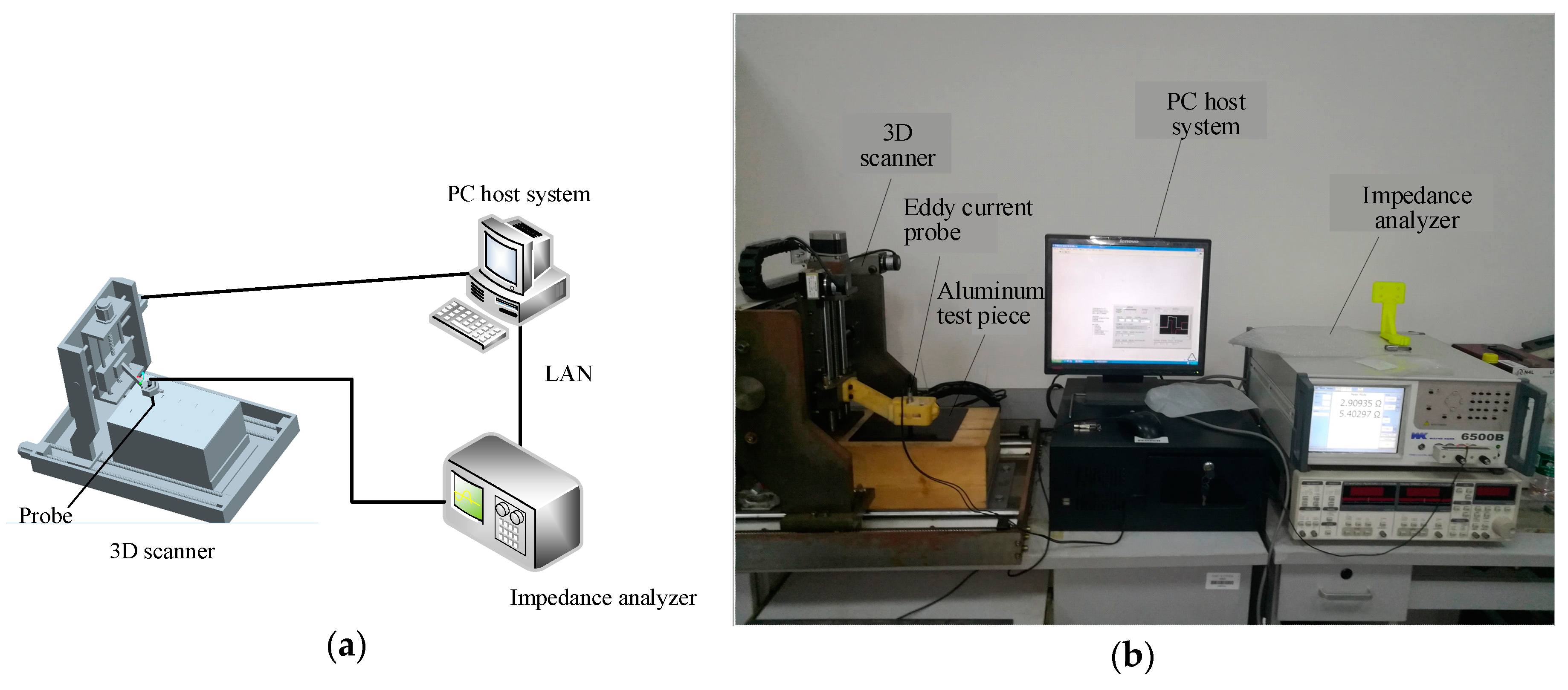
Figure 3 shows the experimental setup, which consists of an eddy current probe, an impedance analyzer, a 3D mobile platform, and a PC host system. The probe is a packaged air-cored coil, and the detailed parameters are shown in

Table 1. Parameters of probe coil.

Parameters	Value
Inner diameter	2.0 mm
Outer diameter	2.4 mm
Distance between coil bottom and specimen surface	1.0 mm
Distance between coil top and specimen surface	6.0 mm
Lift-off (the gap between the coil and specimen)	1.0 mm
Number of turns	300

. The WK65120B impedance analyzer, produced by Wayne Kerr (West Sussex, UK), is used to measure the impedance signal of the probe. Its measuring range is from 20 Hz to 120 MHz, with a 0.05% measuring accuracy. The impedance analyzer communicates with the PC host system through a local area network (LAN). The 3D mobile platform is controlled by pulse width modulation (PWM) signals from a PCI-bus card MPC08, with an application developed in LabVIEW. A pulse from PWM can drive a step motor to rotate on a fixed angle. Therefore, the displacement and the speed of the 3D mobile platform are proportional to the number and frequency of the pulses fed into the motor, respectively. At the same time, the 3D mobile platform is used to place and fix the testing piece and eddy current probe.

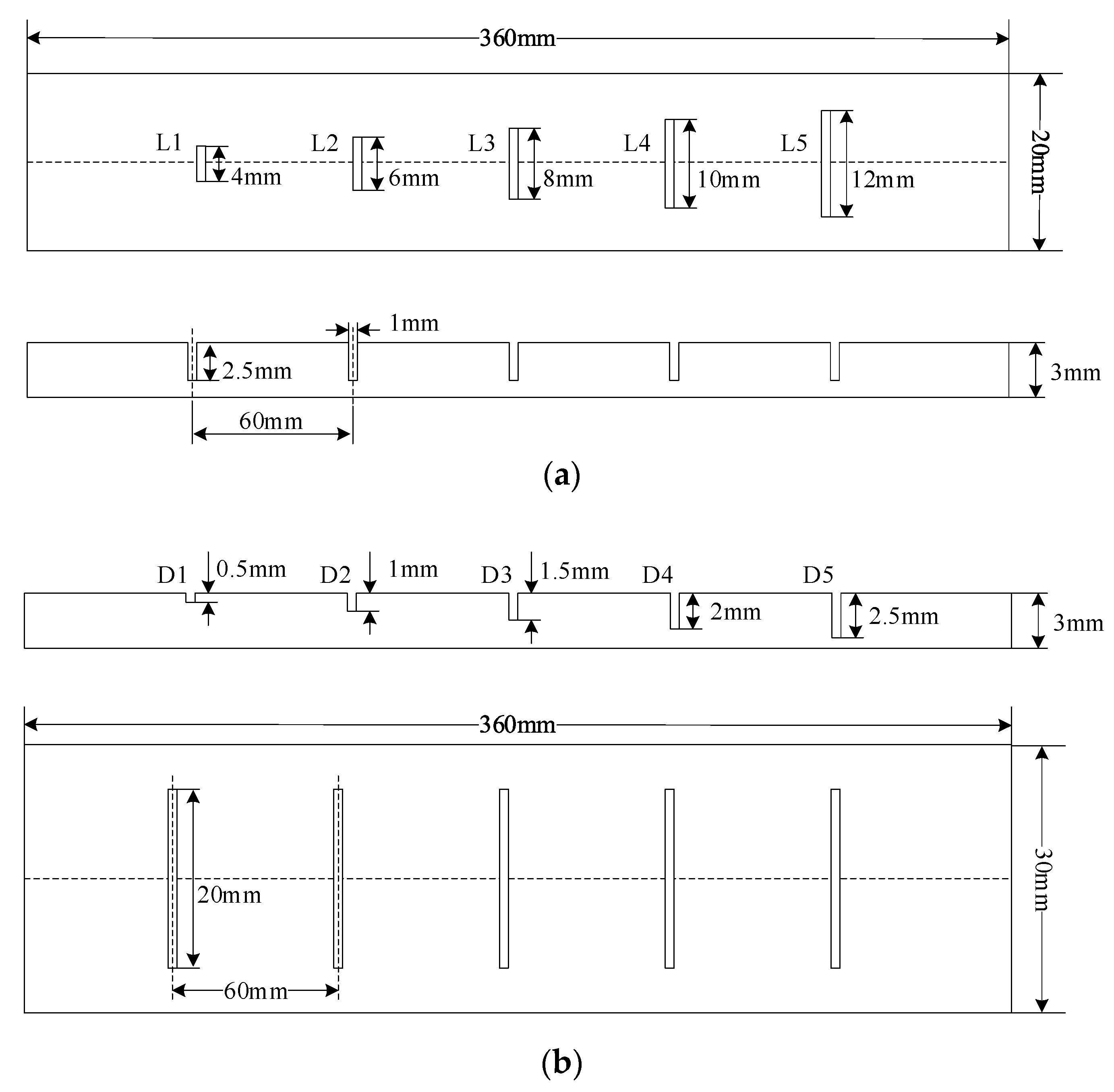
In order to verify the validity of the automatic recognition, classification, and quantitative analysis methods proposed in this paper, ten crack defects of different lengths and depths were manufactured on the surface of a 3 mm thick 6061 aluminum plate by electrical discharge machining, as illustrated in Figure 4. Geometrical parameters of the manufactured crack defects are listed in

Table 2. Metal specimens and defect parameters.

Crack Defects	Specimen Parameters Length × Width × Thickness (mm3)	Defect Length (mm)	Defect Depth (mm)	Defect Width (mm)
L1	360 × 20 × 3	4	2.5	1.0
L2		6
L3		8
L4		10
L5		12
D1	360 × 30 × 3	20	0.5	1.0
D2			1.0
D3			1.5
D4			2.0
D5			2.5

. The five defects have different lengths, ranging from 4 mm to 12 mm, with a step of 2 mm, and width and depth fixed to 1mm and 2.5 mm, respectively. In different length defects, the depth ranges from 0.5 mm to 2.5 mm, with a step of 0.5 mm, and the width and length are fixed to 1 mm and 20 mm, respectively.

4. Results and Discussion

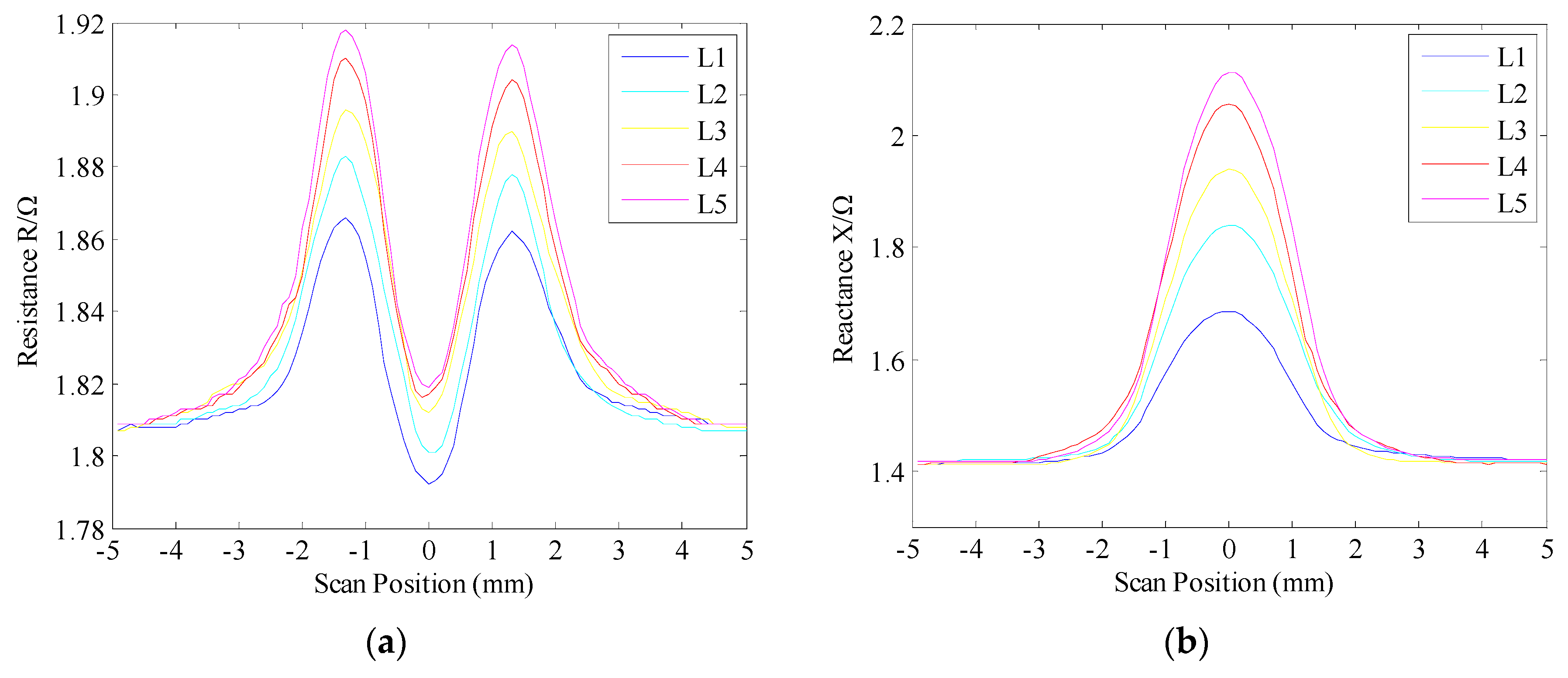
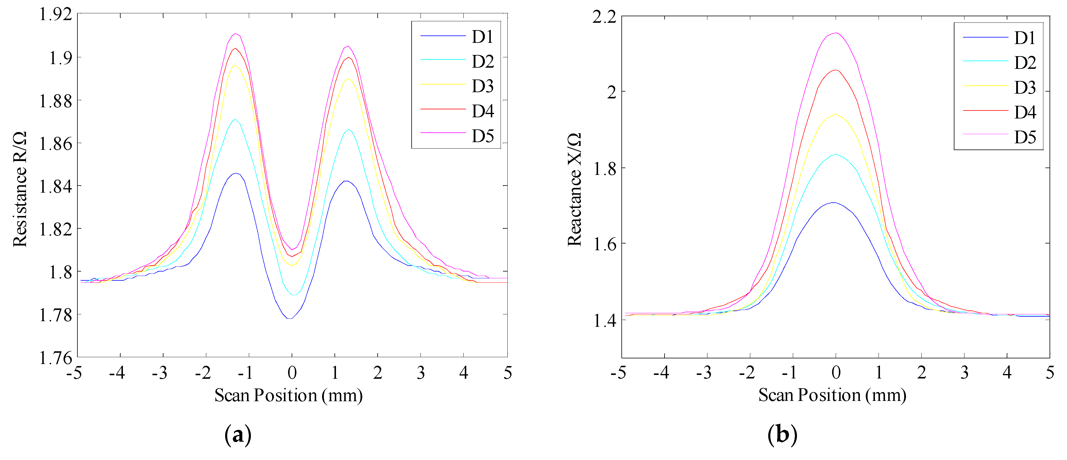
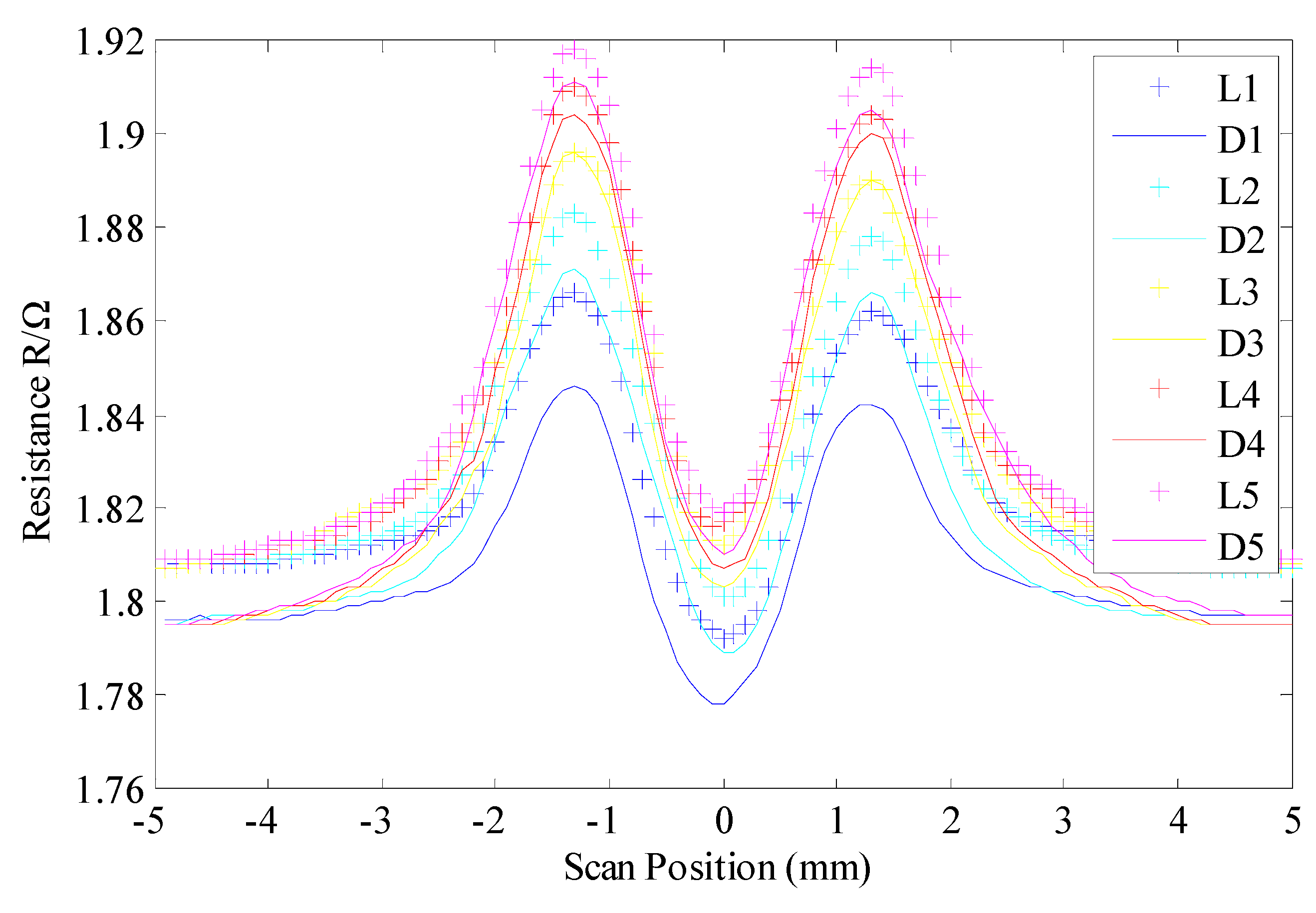
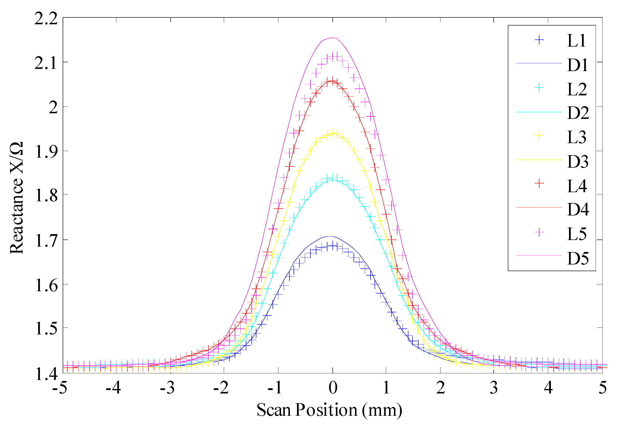
In the experiment, the lift-off of the probe is fixed to 1 mm, and the scanning range in the horizontal direction is set to 10 mm. The scanning step is 0.1 mm, and the scanning speed is 0.1 mm/s, taking the position of the crack defect as the center. Considering the influence of the excitation frequency of the probe in the eddy current testing on the detection depth and sensitivity of the metal specimens, a low excitation frequency leads to a decrease of detection sensitivity, while a high excitation frequency leads to a decrease of detection depth [29]. Therefore, the resistance and reactance information at each scanning point are acquired under the excitation frequency of 450 KHz, and each defect is scanned 10 times. In the experiment, 100 sets of resistance signals and 100 sets of reactance signals of 10 defects were collected. The original resistance and reactance information of the defect are shown in Figure 5 and Figure 6, respectively.

4.1. Original Signal Analysis

As shown in Figure 5 and Figure 6, the x-axis represents the scanning position of the probe, 0 represents the central position of the defect, and the y-axis represents the magnitude of the resistance R and the reactance X, respectively. As the probe approaches the defect, the resistance also increases. When the probe approaches the edge of the defect, the resistance reaches its maximum value, then decreases gradually. When the probe is located at the center of the defect, the resistance decreases to its minimum value, and the probe continues to move from the center of the defect. After leaving the center, the resistance value gradually increases to the maximum, and then decreases after reaching the peak again. Unlike the change of resistance value, the reactance value increases gradually when the probe is near the defect, and reaches the maximum when the probe is located at the defect center; then, the reactance value begins to decrease. During the whole scanning process, there are two peaks in the resistance value, while the reactance value only appears to have one peak at the center of the defect. Figure 6 shows information on the resistance and reactance, which vary with the defect depth, and the variation of the resistance and reactance is the same as that shown in Figure 5.

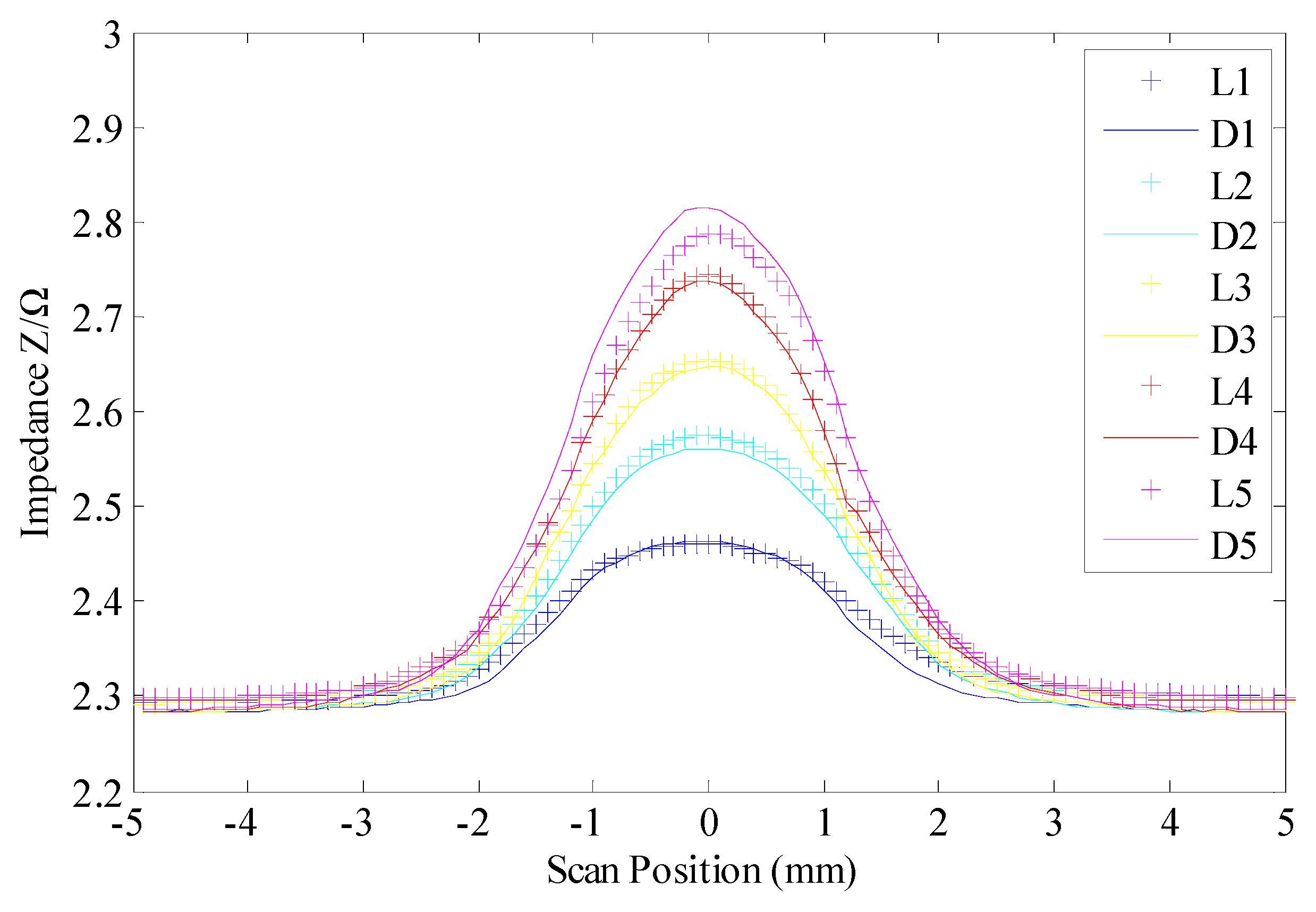
However, the resistance, reactance, and calculated impedance ($\mathrm{Z}=\sqrt{{\mathrm{R}}^2+{\mathrm{X}}^2}$) response of the probe to the length-varying defect and depth-varying defect are very similar, and the detection values at different defect locations overlap to varying degrees. As shown in Figure 7, Figure 8 and Figure 9, the resistance, reactance, and impedance values correspond to the length and depth defects with the same coordinates, respectively. Therefore, if the original signal is directly used to identify and classify defects, it must lead to a misclassification of defects. As shown in

Table 3. Classification results using original signals.

Classifier	Accuracy Rates/%
	Resistance	Reactance	Impedance
Artificial Neural Network	30	26	26
Support Vector Machine	35	30	29
Extreme Learning Machine	60	56	54

, the accuracy rates when the classifiers ANN, SVM, and ELM are used to perform the defect classification, using the original signal as an input feature, are shown. From the classification results, we can see that the classification accuracy of the ELM method is still better than that of ANN and SVM, only when the original signal is used for classification. However, the classification accuracy rate of the three classification methods is less than 60%. Therefore, it is necessary to further extract the features of the original signal in order to improve the accuracy of the detection and classification of defects in metal components.

4.2. Feature Extraction and Classification

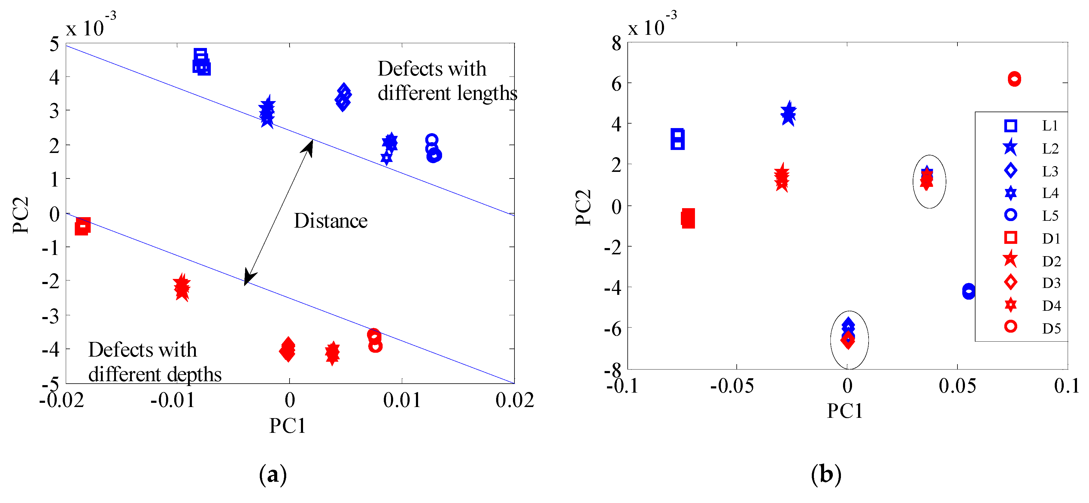
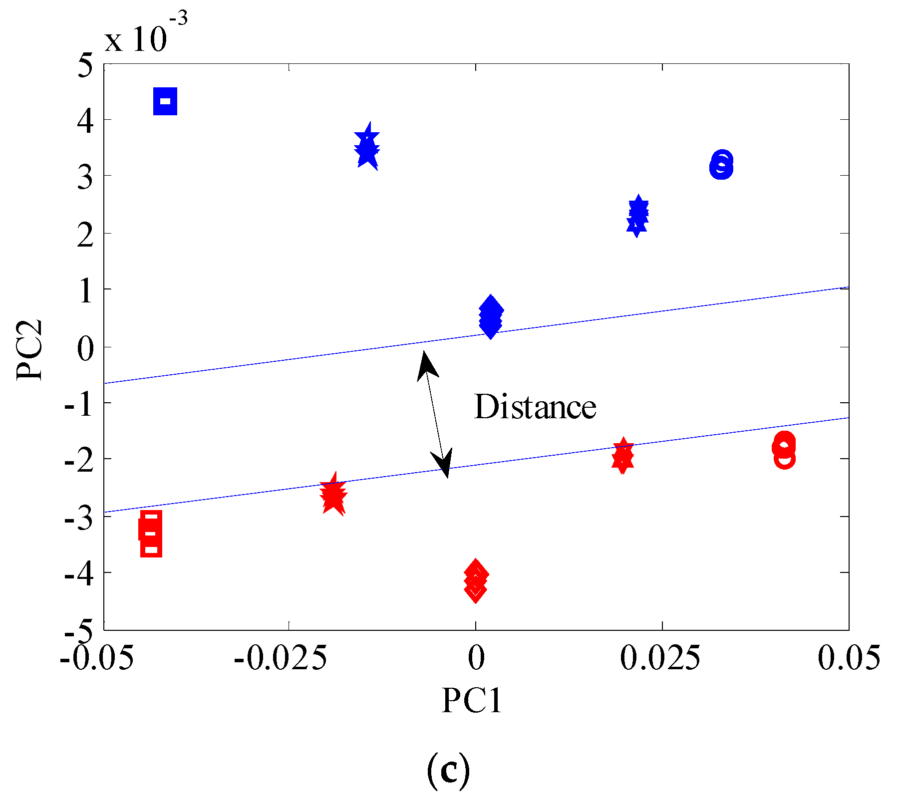
In Section 4.1, it was found that when the original signal is directly used to classify defects, the classification of defects is inaccurate, because the original signal overlaps at different defects to varying degrees. In this subsection, the KPCA algorithm described in Section 2.1 is used to reduce the dimension of the original signal and extract the first four main components as the feature information of defect classification. As shown in Figure 10, the main characteristic distributions of the resistance, reactance, and impedance values of each defect after the feature extraction of KPCA are shown.

As shown in Figure 10a,c, the resistance and impedance of the defects are extracted by the KPCA feature, the length defect and the depth defect features are separated from each other, and there is no feature overlapping phenomenon in different defects. Among them, the length of the resistance feature of the length defect and the depth defect is the largest. However, as shown in Figure 10b, the characteristics of the reactance of each defect still exhibit different degrees of aliasing, particularly defects L3 and D3, L4 and D4. After the feature extraction of KPCA, defects are classified by classifiers ANN, SVM, and ELM. The classification results are shown in

Table 4. Classification results based on Kernel-based Principal Component Analysis feature extraction.

Classifier	Accuracy Rate/%
	Resistance	Reactance	Impedance
Artificial Neural Network	95	70	92
Support Vector Machine	98	75	96
Extreme Learning Machine	100	80	100

, and the accuracy rate of the three classifiers has been significantly improved. The accuracy rate of ELM is 100% when the resistance and impedance eigenvalues are classified, while the accuracy rate of ELM in classifying the reactance eigenvalues is only 80%. However, in the process of defect classification, the larger the feature distance is between the defects, the more favorable is the classification of defects. At the same time, a larger feature distance will give the defect recognition and classification process a higher anti-interference ability and further ensure the accuracy of the automatic defect recognition and classification. Therefore, in this paper and the follow-up research, defect resistance signals will be used to automatically identify and classify defects. In addition, thanks to the single-hidden layer feedforward neural networks of ELM, it is superior to SVM in classification accuracy and generalization [30], and its training time is much lower than that of ANN [19,20].

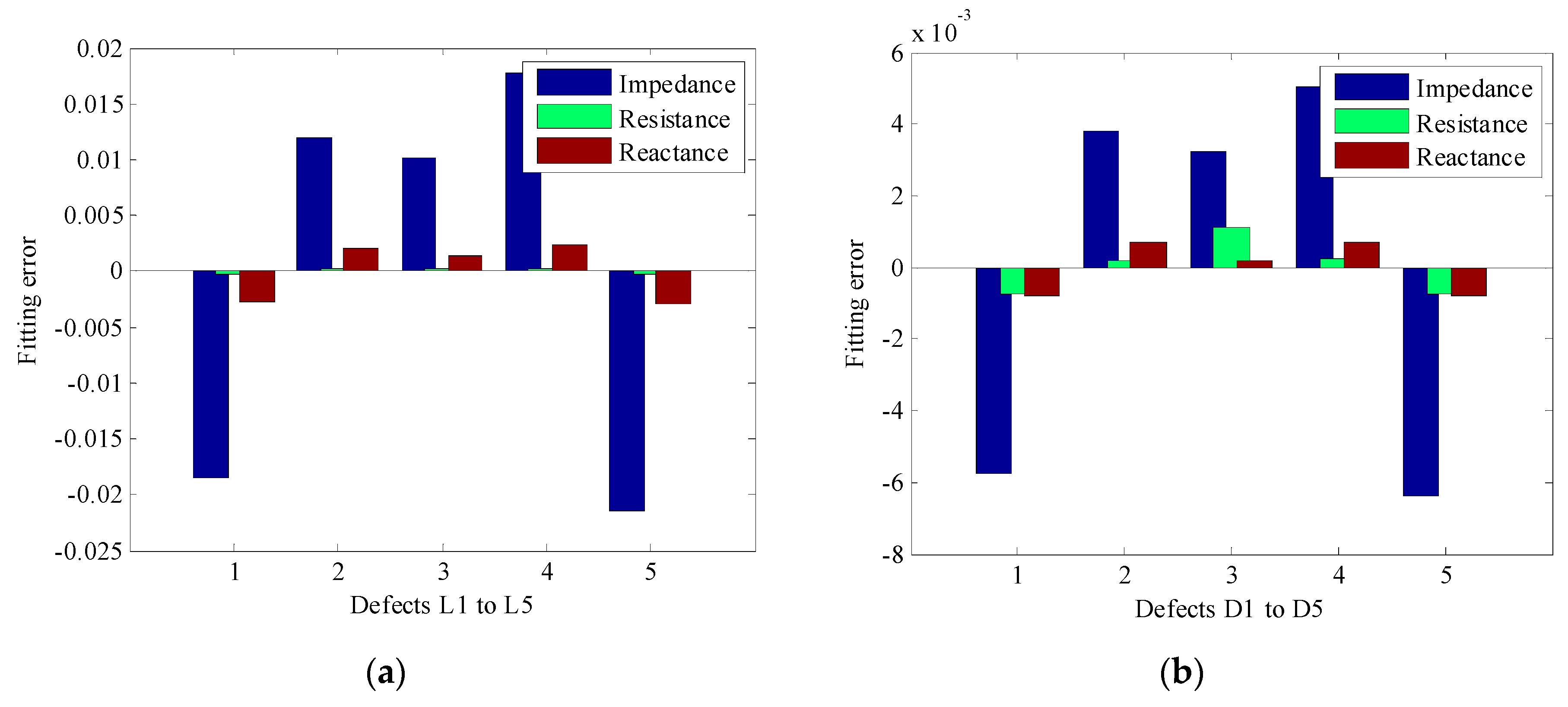
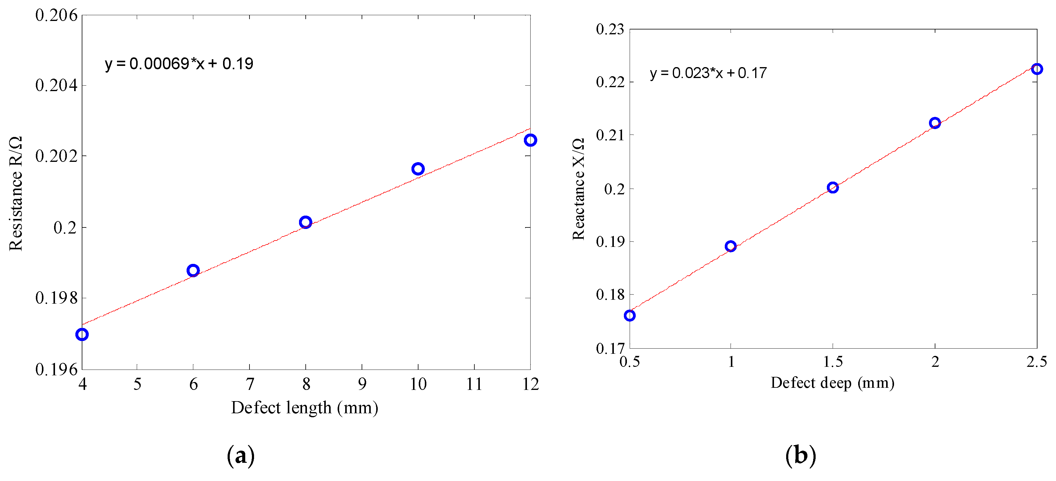
In this paper, the length and depth of defects are fitted by the peak values of the resistance, reactance, and impedance of eddy current signals. Figure 11 shows the fitting errors of eddy current signals for length and depth defects. In relation to the fitting errors of the length defect, the error of the resistance signal is the smallest, at just −0.000253, 0.000158, 0.000148, 0.000243, and −0.000296, followed by the fitting error of the reactance signal, and the fitting error of the impedance signal is the largest in relation to the length defect. In relation to the fitting errors of the depth defect, the reactance signal has the smallest error in each defect, at just −0.000805, 0.000722, 0.000186, 0.000681, and −0.000784, followed by the resistance signal, and the fitting error of the impedance is the largest. Therefore, the resistance and reactance values of the defect signals are used to quantify the length defect and depth defect, respectively. The fitting results are shown in Figure 12. From the fitting results, whether the length of defects is fitted by the resistance value or the depth of defects is fitted by the reactance value, the fitting results maintain a good linear relationship. As shown in Figure 12a, the defect length is fitted by the defect resistance value, and the defect length can be expressed as $y=0.00069*x+0.19$, where $x$ is the measured defect resistance value, and the correlation coefficient is 0.9933. As shown in Figure 12b, the defect depth is fitted by the defect reactance value, and the defect depth can be expressed as $y=0.023*x+0.17$, where $x$ is the measured defect reactance value, and the correlation coefficient is 0.9616.

5. Conclusions and Future Work

The feature of the eddy current signal is extracted by the principal component analysis method based on the kernel function, and the defect eddy current signal is identified and classified by ELM. The experimental results show that the method adopted in this paper has a higher defect classification accuracy than the traditional methods. The following conclusions are drawn from the paper:

• For the defective eddy current signals collected, the resistance signal has the farthest distance between different defects after feature extraction, followed by the impedance signal, while the reactance signal still has aliasing after feature extraction. Therefore, in the process of the eddy current detection of metal component defects, the analysis of resistance signals is more conducive to the identification and classification of defects.
• The method of feature extraction and classification of defective eddy current signals based on KPCA and ELM has a better practicability than traditional methods.
• In the process of fitting defects with linear least squares, the resistance and reactance signal are used to fit the length and depth defect, respectively, as their fitting errors are minimal.

In this paper, the KPCA is used to extract the features of the eddy current signals of defects in metal components, and ELM is used to automatically identify and classify defects, which greatly improves the accuracy of defect classification. At the same time, it provides a new idea for the eddy current testing of defects in metal components and promotes the development of eddy current testing technology. In future research, the author will further expand the scope of defects and increase the complexity of defect composition, the superposition of different defects, and the environmental interference factors, thus broadening the application scope of the proposed method and improving its generalization.

References

1. He, Y.; Luo, F.; Pan, M.; Weng, F.; Hu, X.; Gao, J.; Liu, B. Pulsed eddy current technique for defect detection in aircraft riveted structures. NDT E Int. 2010, 43, 176–181. [Google Scholar] [CrossRef]
2. Angani, C.S.; Park, D.G.; Kim, C.G.; Leela, P.; Kollu, P.; Cheong, Y.M. The pulsed eddy current differential probe to detect a thickness variation in an insulated stainless steel. J. Nondestruct. Eval. 2010, 29, 248–252. [Google Scholar] [CrossRef]
3. Yang, G.; Tamburrino, A.; Udpa, L.; Udpa, S.S.; Zeng, Z.; Deng, Y.; Que, P. Pulsed eddy-current based giant magnetoresistive system for the inspection of aircraft structures. IEEE Trans. Magn. 2010, 46, 910–917. [Google Scholar] [CrossRef]
4. Miorelli, R.; Reboud, C.; Lesselier, D.; Theodoulidis, T. Eddy current modeling of narrow cracks in planar-layered metal structures. IEEE Trans. Magn. 2012, 48, 2551–2559. [Google Scholar] [CrossRef]
5. Yang, R.; He, Y.; Zhang, H. Progress and trends in nondestructive testing and evaluation for wind turbine composite blade. Renew. Sustain. Energy Rev. 2016, 60, 1225–1250. [Google Scholar] [CrossRef]
6. Vavilov, V.P.; Burleigh, D.D. Review of pulsed thermal NDT: Physical principles, theory and data processing. NDT E Int. 2015, 73, 28–52. [Google Scholar] [CrossRef]
7. Lee, K.H.; Baek, M.K.; Park, I.H. Estimation of deep defect in ferromagnetic material by low frequency eddy current method. IEEE Trans. Magn. 2012, 48, 3965–3968. [Google Scholar] [CrossRef]
8. Wang, C.; Fan, M.; Cao, B.; Ye, B.; Li, W. Novel Noncontact Eddy Current Measurement of Electrical Conductivity. IEEE Sens. J. 2018, 18, 9352–9359. [Google Scholar] [CrossRef]
9. Wen, D.; Fan, M.; Cao, B.; Ye, B.; Tian, G. Extraction of LOI Features From Spectral Pulsed Eddy Current Signals for Evaluation of Ferromagnetic Samples. IEEE Sens. J. 2019, 19, 189–195. [Google Scholar] [CrossRef]
10. Ali, K.B.; Abdalla, A.N.; Rifai, D.; Faraj, M.A. Review on system development in eddy current testing and technique for defect classification and characterization. IET Circuits Devices Syst. 2017, 11, 330–343. [Google Scholar] [CrossRef]
11. Bai, L.; Tian, G.Y.; Simm, A.; Tian, S.; Cheng, Y. Fast crack profile reconstruction using pulsed eddy current signals. NDT E Int. 2013, 54, 37–44. [Google Scholar] [CrossRef]
12. Chen, H.; Wang, C.; Zuo, X. Research on methods of defect classification based on metal magnetic memory. NDT E Int. 2017, 92, 82–87. [Google Scholar] [CrossRef]
13. Li, K.; Ma, Z.; Fu, P.; Krishnaswamy, S. Quantitative evaluation of surface crack depth with a scanning laser source based on particle swarm optimization-neural network. NDT E Int. 2018, 98, 208–214. [Google Scholar] [CrossRef]
14. Rowshandel, H.; Nicholson, G.L.; Shen, J.L.; Davis, C.L. Characterisation of clustered cracks using an ACFM sensor and application of an artificial neural network. NDT E Int. 2018, 98, 80–88. [Google Scholar] [CrossRef]
15. He, Y.; Pan, M.; Chen, D.; Luo, F. PEC defect automated classification in aircraft multi-ply structures with interlayer gaps and lift-offs. NDT E Int. 2013, 53, 39–46. [Google Scholar] [CrossRef]
16. Chen, T.; Tian, G.Y.; Sophian, A.; Que, P.W. Feature extraction and selection for defect classification of pulsed eddy current NDT. NDT E Int. 2008, 41, 467–476. [Google Scholar] [CrossRef]
17. Chen, X.; Hou, D.; Zhao, L.; Huang, P.; Zhang, G. Study on defect classification in multi-layer structures based on Fisher linear discriminate analysis by using pulsed eddy current technique. NDT E Int. 2014, 67, 46–54. [Google Scholar] [CrossRef]
18. Peng, Y.; Qiu, X.; Wei, J.; Li, C.; Cui, X. Defect classification using PEC respones based on power spectral density analysis combined with EMD and EEMD. NDT E Int. 2016, 78, 37–51. [Google Scholar] [CrossRef]
19. Rosado, L.S.; Janeiro, F.M.; Ramos, P.M.; Piedade, M. Defect Characterization with Eddy Current Testing Using Nonlinear-Regression Feature Extraction and Artificial Neural Networks. IEEE Trans. Instrum. Meas. 2013, 62, 1207–1214. [Google Scholar] [CrossRef]
20. Postolache, O.; Ramos, H.G.; Ribeiro, A.L. Detection and characterization of defects using GMR probes and artificial neural networks. Comput. Stand. Interfaces 2011, 33, 191–200. [Google Scholar] [CrossRef]
21. Hu, J.; Xu, W.; Gao, B.; Tian, G.; Wang, Y.; Wu, Y.; Yin, Y.; Chen, J. Pattern Deep Region Learning for Crack Detection in Thermography Diagnosis System. Metals 2018, 8, 612. [Google Scholar] [CrossRef]
22. Xu, Y.; Ran, J.; Chen, H. Kohonen neural network classification for failure process of metallic organic coating in corrosion environment. Metals 2017, 7, 147. [Google Scholar]
23. Huang, G.B.; Zhu, Q.Y.; Siew, C.K. Extreme learning machine: Theory and applications. Neurocomputing 2006, 70, 489–501. [Google Scholar] [CrossRef] [Green Version]
24. Huang, G.B.; Zhou, H.; Ding, X.; Zhang, R. Extreme learning machine for regression and multiclass classification. IEEE Trans. Syst. Man Cybern. Part B 2012, 42, 513–529. [Google Scholar] [CrossRef] [PubMed]
25. Wang, Y.; Cao, F.; Yuan, Y. A study on effectiveness of extreme learning machine. Neurocomputing 2011, 74, 2483–2490. [Google Scholar] [CrossRef] [Green Version]
26. Schölkopf, B.; Smola, A.; Müller, K.R. Kernel principal component analysis. In International Conference on Artificial Neural Networks; Springer: Berlin/Heidelberg, Germany, 1997; pp. 583–588. [Google Scholar]
27. Lee, J.M.; Yoo, C.; Choi, S.W.; Vanrolleghem, P.A.; Lee, I.B. Nonlinear process monitoring using kernel principal component analysis. Chem. Eng. Sci. 2004, 59, 223–234. [Google Scholar] [CrossRef]
28. Ye, B.; Huang, P.; Fan, M.; Gong, X.; Hou, D.; Zhang, G.; Zhou, Z. Automatic classification of eddy current signals based on kernel methods. Nondestruct. Test. Eval. 2009, 24, 19–37. [Google Scholar] [CrossRef]
29. Ding, S.; Zhao, H.; Zhang, Y.; Xu, X.; Nie, R. Extreme learning machine: Algorithm, theory and applications. Artif. Intell. Rev. 2015, 44, 103–115. [Google Scholar] [CrossRef]
30. Fan, M.; Wang, Q.; Cao, B.; Ye, B.; Sunny, A.I.; Tian, G. Frequency optimization for enhancement of surface defect classification using the eddy current technique. Sensors 2016, 16, 649. [Google Scholar] [CrossRef]
Figure 1. Extreme Learning Machine (ELM) schematic diagram.
Metals 09 00155 g001
Figure 2. The flowchart of the automatic identification, classification, and quantitative analysis of defects in metal components.
Metals 09 00155 g002
Figure 3. Experimental setup. Schematic diagram (a) and Practical setup (b).
Metals 09 00155 g003
Figure 4. Fabricated specimens. Crack defects with different lengths (a) and different depths (b).
Metals 09 00155 g004
Figure 5. Variation of resistance (a) and reactance (b) with defect length.
Metals 09 00155 g005
Figure 6. Variation of resistance (a) and reactance (b) with defect width.
Metals 09 00155 g006
Figure 7. Variation of resistance with defect length and depth.
Metals 09 00155 g007
Figure 8. Variation of reactance with defect length and depth.
Metals 09 00155 g008
Figure 9. Variation of impedance with defect length and depth.
Metals 09 00155 g009
Figure 10. Distribution of the two principal components of the resistance signal (a), reactance signal (b), and impedance signal (c).
Metals 09 00155 g010aMetals 09 00155 g010b
Figure 11. Fitting error of the length defect (a) and the width defect (b).
Metals 09 00155 g011
Figure 12. Fitting results of the length defect (a) and the width defect (b).
Metals 09 00155 g012