Article

A Fast Method for Predicting the Mechanical Properties of Precipitation-Hardenable Aluminum Alloys

Leibniz Institute for Materials Engineering IWT, University of Bremen, Badgasteiner Str. 3, 28359 Bremen, Germany
*
Author to whom correspondence should be addressed.
Metals 2019, 9(2), 147; https://doi.org/10.3390/met9020147
Submission received: 7 December 2018 / Revised: 18 January 2019 / Accepted: 25 January 2019 / Published: 29 January 2019

Abstract

:
Most heat treatment simulations of precipitation-hardenable aluminum alloys are incomplete or restricted to sub-steps of the process chain. In general, the studies addressing the heat treatment of aluminum components have only provided a qualitative guidance of heat treatment, which does not match the heat treatment that is necessary for specific parts with specific requirements. Thus, a quick and accurate simulation of the whole heat treatment process would hold great economic benefit for industrial applications in predicting suitable heat treatment processes that are able to meet the required mechanical properties of proposed novel aluminum components. In this paper, the development of a time and cost efficient method for generating such prediction models is presented by means of an example aluminum alloy EN AW-6082. During the process sub-steps of solution annealing, quenching and aging, the time-temperature correlations connected to the precipitation-hardening conditions were analyzed. The precision of the prediction model depends on the size of the material database, which should be able to be adjusted to the individual requirements of the simulation user. In order to obtain the greatest time and cost efficiency in generating such a model, a specific experimental design was developed. The results of the method development are presented and discussed.

1. Introduction

In the production of aluminum components from heat-treatable alloys, precipitation hardening represents a major process step in the final adjustment and improvement of the mechanical properties. In general, it is subdivided into the different sub-steps of “solution annealing”, “quenching” and “aging”.
Various models exist for the phase developments during the precipitation hardening of aluminum alloys, which are predominantly based on metal–physical interrelations. They are often very complex and require exact knowledge of the chemical composition of the alloy and the material conditions. In many cases, their transferability to other materials is severely limited due to the direct dependence of the models on the initial microstructure and the alloying elements. The determination of the required input variables is often carried out by using specific experimental methods, such as small-angle X-ray scattering [1,2], small-angle neutron scattering [3], transmission electron microscopy [2,3,4,5,6] or differential scanning calorimetry [5,7]. These methods, which are additionally used to validate the simulation models, require high technical effort and specific sample preparation. Typical output variables from the modeling of the precipitation hardening include the number [1,8] and the average diameter of certain phases [2,5,8,9] or their volume fraction in the structure [1,4,10,11,12].
The microstructure development of the heat-treated parts during the precipitation hardening forms the basis for determining the changes in mechanical properties. The parameters of the strength-enhancing phases, such as size, number and/or distribution, are often used as input variables for the prediction of the firmness irrespective of whether they are of experimental or simulative origin. In many cases, the basic equations of solid solution strengthening and precipitation hardening are used to calculate the yield and tensile strength and hardness. [4,5,7,13,14].
Kinetic models based on CALPHAD (CALculation of PHAse Diagrams) have proven to be very effective. However, when using thermodynamic databases, care must be taken to ensure that the database used is capable of correctly reproducing the desired system [15,16]. One of the methods often used for the development of models in materials science is TEP (Thermodynamic Extremal Principle) which is based on thermodynamic calculations. The TEP is a useful tool for the solution of practical problems of the thermodynamics of irreversible processes, but the basis for the calculation of the thermodynamics of the system are CALPHAD databases, providing chemical potentials of the phases as well as diffusivities of the involved elements on the basis of the chemical composition of the alloy and the present temperature [17].
In addition to models based on strength-enhancing phase developments, which are highly limited in their ability to rapidly evaluate the effects of precipitation-hardening conditions on component strength due to their high technical complexity, models have been established that provide a direct correlation between precipitation-hardening parameters and mechanical properties. All these models include only one step of the precipitation hardening process, such as the model for calculating the dependency of the tension–strain relation on the solution annealing time of an EN AW 6082 alloy [18]. With regards to quenching, the Quench Factor Analysis (QFA) method for determining mechanical properties according to the quenching speed has been successfully used for several decades for various aluminum alloys [19,20,21,22,23] and has been implemented in Finite Element applications [24,25,26]. The analysis is based on the mathematical calculation of the hardness reduction due to the phases, which have already formed during quenching, without direct analysis of the properties of these phases. Hardness was also calculated using a relatively simple relationship that depends on the quenching rate, aging temperature and aging time [27].
In the industrial settings, an “ideal” heat treatment of aluminum components is often difficult to implement in a way that is similar to how it is commonly described in literature. Among others, these difficulties are due to the diverse differences between industrial circumstances and laboratory conditions. Thus far, none of the models described have been able to realize the direct connection of the relationships between time, temperature and mechanical properties, which are known from experimental investigations, with simple mathematical descriptions and without detailed knowledge of the present microstructure.
This publication describes a fast method, by which a model for predicting the mechanical properties of heat-treatable aluminum alloys can be generated with low experimental effort. In addition to having a sufficiently high calculation accuracy, this model has the required rapidity. This method is particularly important for new alloys that cannot be described with the current CALPHAD database.

2. Materials and Methods

2.1. Material and Samples

The method was developed by means of an example aluminum alloy EN AW-6082. The experiments were performed with flat specimens with a thickness of 2.5 mm. The chemical composition of the alloy was measured by glow discharge optical emission spectroscopy (GDOES). The results are presented in Table 1.

2.2. Experimental Design and Measurements

The designing of the experiments and data analysis was conducted using Cornerstone® software (version 7.1.0.2, camLine GmbH, Petershausen, Germany). The variation of heat treatment parameters was carried out according to the D-Optimal experimental design [28]. The advantages of a D-Optimal experimental design included significantly reduced experimental effort and maximum prediction power in the selected range of the parameters. In addition, an already performed experimental plan could be subsequently expanded by further experiments. Besides, parameter settings could be left out of the model if these were not important or unrealistic. In this present study, the parameters of solution annealing temperature and times as well as quenching medium and aging temperature and duration were varied (Table 2).
When creating the D-Optimal experimental design, a quadratic regression model with five linear terms (Ts, ts, QM, Ta, ta), ten interaction terms (Ts × ts, Ts × QM, Ts × Ta, Ts × ta, ts × QM, ts × Ta, ts × ta, QM × Ta, QM × ta, Ta × ta) and four quadratic terms (Ts2, ts2, Ta2, ta2) was assumed. In this case, 25 experiments were needed to create the regression model. This number of experiments was extended to 30 to increase the accuracy. The experiments designed with the Cornerstone® are listed in Table 3.
To determine the time-temperature curves within the samples and to ensure a homogeneous temperature distribution, the accompanying thermocouple measurements were obtained in all experiments.
After heat treatment, hardness and electrical conductivity were measured and quasi-static tensile tests were carried out. Electrical conductivity measurements were conducted using a portable electrical conductivity measurement device (SIGMASCOPE® SMP350, Fischer Technology Inc., Windsor, CT, USA). The number of the measurements of the electrical conductivity per sample varied between five and ten measured values depending on the scattering of the individual samples. Vickers hardness measurements were performed with a load of 5 kp. The hardness measurements on the sheet samples were carried out with five individual measurements per part.

3. Results and Discussion

By using the D-optimal experimental design, a wide spectrum of heat treatment conditions could be investigated with low experimental effort. In the case of five factors and three variations, the D-Optimal design required only thirty trials. In comparison, a full factorial design would consist of three to the power of five (243) experiments. However, using the D-Optimal experimental design, the choice of examination area was of particular importance.
The mean values of results for hardness and electrical conductivity of the flat samples are shown in Figure 1. The heat treatment parameters can be taken from Table 3 according to the numbers of the experiments. The measured hardness of the flat samples varied between 57.16 HV5 and 119.40 HV5. The electrical conductivity fluctuated between 24.26 MS/m and 30.26 MS/m.
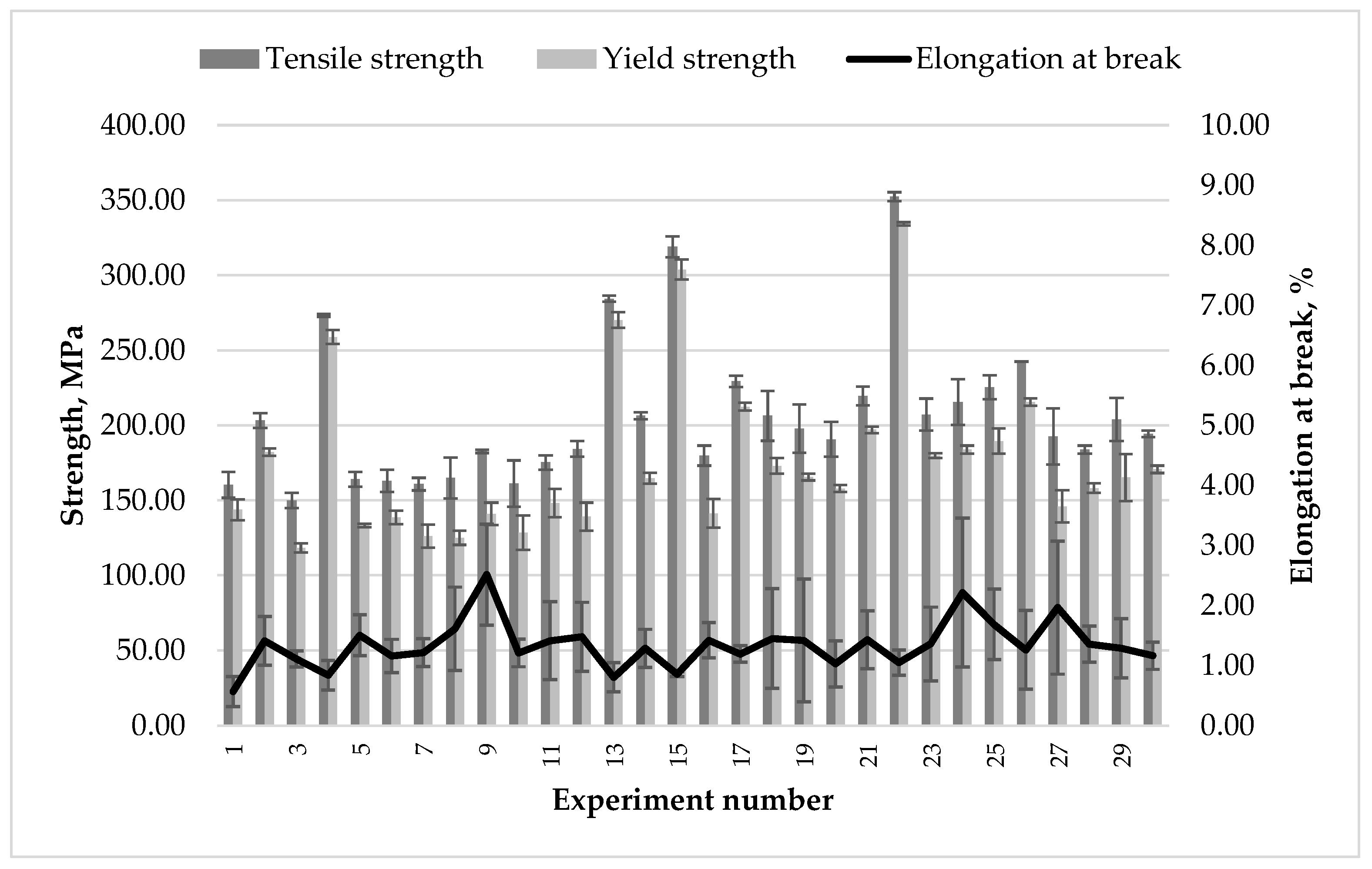
Figure 2 shows the mean values and standard deviation of the measurements of tensile strength, yield strength and elongation at break from the 30 heat treatments. The experiment numbers were identical to the numbers in Figure 1 and Table 3.
The correlation between hardness and tensile strength was as expected. As a side effect, this method accurately determined the coefficient for converting hardness into tensile strength. The conversion did not become more accurate, however, if the electrical conductivity was taken as the predictor factor. This was because in the considered range of the experimental investigations, the results of both strongly underaged and overaged states were included.
The summary of the significance values of the predictors is shown in Table 4. It gives a quick overview of the regression model. For example, aging temperature, aging temperature to the square, aging time and aging temperature multiplied by aging time had the greatest impact on the hardness. The solution annealing temperature, solution annealing time and quenching medium had only a small effect on the hardness. In contrast, the electrical conductivity depended mainly on the solution annealing temperature and quenching medium.
In the selected experimental area for most properties, the multiple linear regression model with quadratic terms and interactions between variables achieved an accuracy of 95%. Table 4 summarizes the achieved values of adjusted coefficient of determination (adjusted R-squared), which is a modified version of the coefficient of determination (R-squared) adjusted to the number of predictors in the model, for the measured properties. From the values in Table 4, all measured properties except for elongation at break could be calculated with high accuracy using the selected heat treatment parameters. The elongation at break was largely determined by the presence of defects. This information was not available from the heat treatment parameters and thus, it was not possible to calculate the elongation at break from statistical correlations of the described method.
The mechanical properties in the selected heat treatment range were calculated as follows:
Hardness (HV5) = −1609.84183 + Ts × 5.501569951 − ts × 0.34601087 + QMgas × 33.16496749 − QMpolymer × 32.59246355 − QMwater × 0.572503942 + Ta × 2.422517718 + ta × 1.304904475 − Ts2 × 0.005023035 − QMgas × Ts × 0.066910132 + QMpolymer × Ts × 0.066563025 + QMwater × Ts × 0.000347107 − QMgas × ts × 0.045869782 − QMpolymer × ts × 1.230807755 + QMwater × ts × 1.276677537 − Ta2 × 0.006914451 − ta × Ta × 0.006998195
Electrical conductivity (MS/m) = 36.2261029 − Ts × 0.0237104 + ts × 0.4989135 + QMgas × 0.3737312 − QMpolymer × 0.1528800 − QMwater × 0.2208513 + Ta × 0.0082265 + ta × 0.0156832 − ts2 × 0.1103598 + Ta2 × 0.0000561
Yield strength (MPa) = −6897.6096149 + Ts × 23.2700403 − QMgas × 11.4006131 + QMpolymer × 3.7195440 + QMwater × 7.6810691 + Ta × 10.0708414 + ta × 0.3706790 − Ts2 × 0.0213418 − Ta2 × 0.0285358 − ta × Ta × 0.0204646 + ta2 × 0.1214644
Tensile strength (MPa) = −6603.1500875 + Ts × 22.6267057 − QMgas × 11.6506298 + QMpolymer × 2.9249364 + QMwater × 8.7256935 + Ta × 8.8145630 + ta × 2.4305712 − Ts2 × 0.0207380 − Ta2 × 0.0251695 − ta × Ta × 0.0161967
Elongation at break (%) = −5.8839467 + Ts × 0.0181320 + ts × 1.3475997 + Ta × 0.0027528 + ta × 0.0632576 − ts × Ts × 0.0025377 − Ta × Ts × 0.0000732 + ta × ts × 0.0070746 + Ta2 × 0.0001046 + ta × Ta × 0.0001821 − ta2 × 0.0048555
QM is equal to 1 for the used quenching medium and 0 for all others.
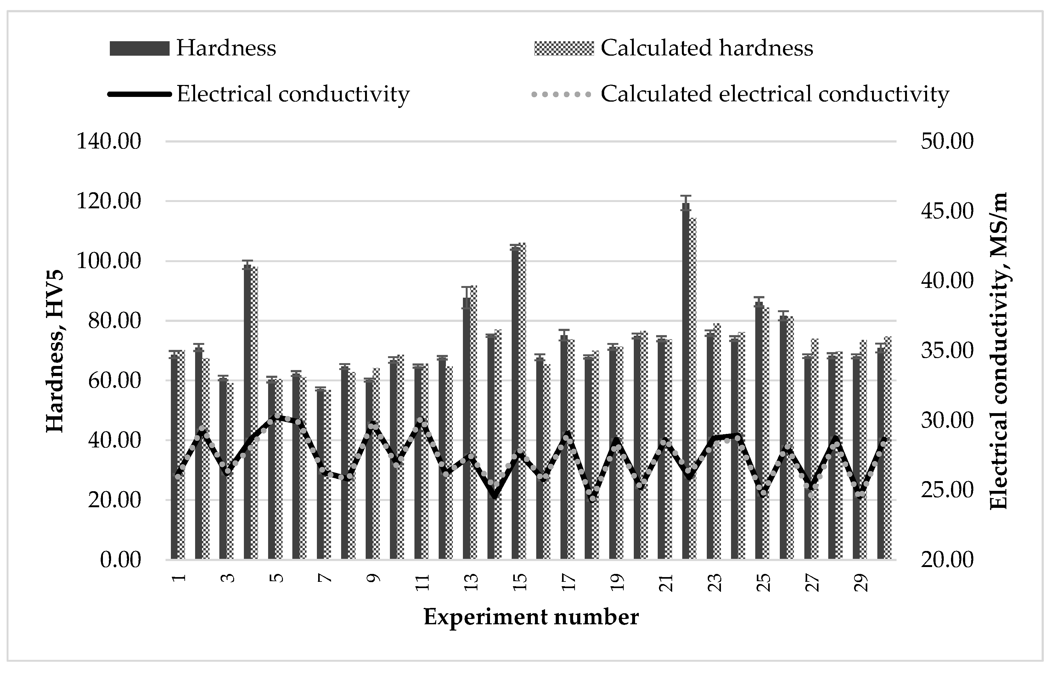
The easily interpretable graphical comparison of the experimental and calculated data for the hardness and electrical conductivity is shown in Figure 3. The calculations were carried out with the heat treatment parameters used to create the regression model. It can be seen that a good agreement between experiment and calculation was reached.

4. Conclusions and Outlook

In this paper, a method to develop a model for the fast and sufficiently accurate computation of the mechanical properties after the heat treatment (i.e., solution annealing, quenching and aging) of age-hardenable aluminum alloys using time-temperature relations was presented. The developed method was suitable for rapid determination of the properties of such aluminum alloys, in which the experimental effort was significantly reduced by using a D-optimal experimental design. The accuracy of the results depended on the selected limitation of the parameter range for heat treatment. In the selected experimental area for hardness, electrical conductivity, yield strength and tensile strength the regression model achieved an accuracy of 95%. In the case where the minimum quantity of data had been determined only, the mechanical properties of various heat treatment conditions could be merely converted into one another. In the next step, the data basis had to be extended and the resulting model had to be transferred to complex parts in order to prove its general applicability. The transition from the flat specimens to the real components would be achieved with the results of the Jominy tests. This simple test established the relationship of the cooling rate (distance from quenched end) with local hardness and local electrical conductivity. With a lower cooling rate, or a greater distance from the quenched end, the hardness decreased and the electrical conductivity increased. At the maximum distance from the quenched end, the Jominy samples had minimal hardness and maximal electrical conductivity. In this way, the relationship between the distance from the quenched end or thickness of the sample and the electrical conductivity and hardness could be established.

Author Contributions

A.T. performed all experiments, analyzed the obtained data and wrote the paper. A.v.H. supervised all investigations, supported the work with his scientific knowledge and supplemented the publication with conclusions at a higher level.

Funding

The IGF Project (18641 N) of the Arbeitsgemeinschaft Wärmebehandlung und Werkstofftechnik e. V. (AWT) was funded by the Arbeitsgemeinschaft industrieller Forschungsvereinigungen “Otto von Guericke” e. V. (AiF) through the IGF program of the Bundesministerium für Wirtschaft und Energie (BMWi) due to a resolution of the Deutscher Bundestag. The authors are grateful for the financial support.

Acknowledgments

We further wish to thank the Expert Committee 24 “Wärmebehandlung von Nichteisenmetallen” of AWT for scientific support and supervision of the project.

Conflicts of Interest

The authors declare no conflict of interest.

References

  1. Nicolas, M.; Deschamps, A. Characterisation and modelling of precipitate evolution in an Al-Zn-Mg alloy during non-isothermal heat treatments. Acta Mater. 2003, 51, 6077–6094. [Google Scholar] [CrossRef]
  2. Werenskiold, J.C.; Deschamps, A.; Brechet, Y. Characterization and modeling of precipitation kinetics in an Al-Zn-Mg alloy. Mater. Sci. Eng. 2000, A293, 267–274. [Google Scholar] [CrossRef]
  3. Bardel, D.; Perez, M.; Nelias, D.; Deschamps, A.; Hutchinson, C.R.; Maisonnette, D.; Chaise, T.; Garnier, J.; Bourlier, F. Coupled precipitation and yield strength modelling for non-isothermal treatments of a 6061 aluminium alloy. Acta Mater. 2014, 62, 129–140. [Google Scholar] [CrossRef] [Green Version]
  4. Esmaeili, S.; Lloyd, D.J. Modeling of precipitation hardening in pre-aged AlMgSi(Cu) alloys. Acta Mater. 2005, 53, 5257–5271. [Google Scholar] [CrossRef]
  5. Khan, I.N.; Starink, M.J.; Yan, J.L. A model for precipitation kinetics and strengthening in Al-Cu-Mg alloys. Mater. Sci. Eng. 2008, A472, 66–74. [Google Scholar] [CrossRef]
  6. Österreicher, J.A.; Papenberg, N.P.; Kumar, M.; Ma, D.; Schwarz, S.; Schlögl, C.M. Quantitative prediction of the mechanical properties of precipitation-hardened alloys with special application to Al-Mg-Si. Mater. Sci. Eng. A 2017, 703, 380–385. [Google Scholar] [CrossRef]
  7. Sepehrband, P.; Esmaeili, S. Application of recently developed approaches to microstructural characterization and yield strength modeling of aluminum alloy AA7030. Mater. Sci. Eng. A 2008, 487, 309–315. [Google Scholar] [CrossRef]
  8. Zhu, A.W.; Starke, E.A., Jr. Stress aging of Al-Cu alloys: Computer modeling. Acta Mater. 2001, 49, 3063–3069. [Google Scholar] [CrossRef]
  9. Jiang, H.; Faulkner, R.G. Modelling of grain boundary segregation, precipitation and precipitate-free zones of high strength aluminium alloys—I. The model. Acta Mater. 1996, 44, 1857–1864. [Google Scholar] [CrossRef]
  10. Khan, I.N.; Starink, M.J. Microstructure and strength modelling of Al-Cu-Mg alloys during non-isothermal treatments Part 1—Controlled heating and cooling. Mater. Sci. Technol. 2008, 24, 1403–1410. [Google Scholar] [CrossRef]
  11. Löchte, L.; Gitt, A.; Gottstein, G.; Hurtado, I. Simulation of the evolution of GP zones in Al-Cu alloys: An extended Cahn-Hilliard approach. Acta Mater. 2000, 48, 2969–2984. [Google Scholar] [CrossRef]
  12. Robson, J.D. A new model for prediction of dispersoid precipitation in aluminium alloys containing zirconium and scandium. Acta Mater. 2004, 52, 1409–1421. [Google Scholar] [CrossRef]
  13. Esmaeili, S.; Lloyd, D.J.; Poole, W.J. A yield strength model for the Al-Mg-Si-Cu alloy AA6111. Acta Mater. 2003, 51, 2243–2257. [Google Scholar] [CrossRef]
  14. Zander, J.; Sandström, R. One parameter model for strength properties of hardenable aluminium alloys. Mater. Des. 2008, 29, 1540–1548. [Google Scholar] [CrossRef]
  15. Zhang, X.; Wang, H.; Kuang, W.; Zhang, J. Application of the thermodynamic extremal principle to phase-field modeling of non-equilibrium solidification in multi-component alloys. Acta Mater. 2017, 128, 258–267. [Google Scholar] [CrossRef]
  16. Liu, S.; Gao, M.C.; Liaw, P.K.; Zhang, Y. Microstructures and mechanical properties of AlxCrFeNiTi0.25 alloys. J. Alloy. Compd. 2015, 619, 610–615. [Google Scholar] [CrossRef]
  17. Lang, P.; Povoden-Karadeniz, E.; Falahati, A.; Kozeschnik, E. Simulation of the effect of composition on the precipitation in 6xxx Al alloys during continuous-heating DSC. J. Alloy. Compd. 2014, 612, 443–449. [Google Scholar] [CrossRef]
  18. Garrett, R.P.; Lin, J.; Dean, T.A. An investigation of the effects of solution heat treatment on mechanical properties for AA 6xxx alloys: Experimentation and modelling. Int. J. Plast. 2005, 21, 1640–1657. [Google Scholar] [CrossRef]
  19. Bates, C.E. Quench optimization for aluminum alloys. AFS Trans. 1994, 93–25, 1045–1054. [Google Scholar]
  20. Flynn, R.J.; Robinson, J.S. The application of advances in quench factor analysis property prediction to the heat treatment of 7010 aluminium alloy. J. Mater. Process. Technol. 2004, 153–154, 674–680. [Google Scholar] [CrossRef]
  21. Ma, S.; Maniruzzaman, M.D.; MacKenzie, D.S.; Sisson, R.D., Jr. A methodology to predict the effects of quench rates on mechanical properties of cast aluminum alloys. Metall. Mater. Trans. 2007, 38B, 583–589. [Google Scholar] [CrossRef]
  22. Rometsch, P.A.; Schaffer, G.B.; Yao, J.-Y.; Couper, M.J. Application of quench factor analysis to A356.0 and A357.0 foundry alloys. In Proceedings of the 6th International Conference on Aluminum Alloys, Toyohashi, Japan, 5–10 July 1998. [Google Scholar]
  23. Staley, J.T. Quench factor analysis of aluminium alloys. Mater. Sci. Technol. 1987, 3, 923–935. [Google Scholar] [CrossRef]
  24. Dolan, G.P.; Flynn, R.J.; Tanner, D.A.; Robinson, J.S. Quench factor analysis of aluminium alloys using Jominy end quench technique. Mater. Sci. Technol. 2005, 21, 687–692. [Google Scholar] [CrossRef]
  25. Järvsträt, N.; Tjøtta, S. Modelling cooling of aluminium extrusions. In Proceedings of the Abaqus Users’ Conference, Newport, RI, USA, 19–22 May 1994; pp. 307–316. [Google Scholar]
  26. Robinson, J.S.; Cudd, R.L.; Tanner, D.A.; Dolan, G.P. Quench sensitivity and tensile property inhomogeneity in 7010 forgings. J. Mater. Process. Technol. 2001, 119, 261–267. [Google Scholar] [CrossRef] [Green Version]
  27. Güzel, A.; Jäger, A.; Ben Khalifa, N.; Tekkaya, A.E. Simulation of the quench sensitivity of the aluminum alloy 6082. Key Eng. Mater. 2010, 424, 51–56. [Google Scholar] [CrossRef]
  28. Box, G.E.P.; Lucas, H.L. Design of experiments in nonlinear situations. Biometrika 1959, 46, 77–90. [Google Scholar] [CrossRef]
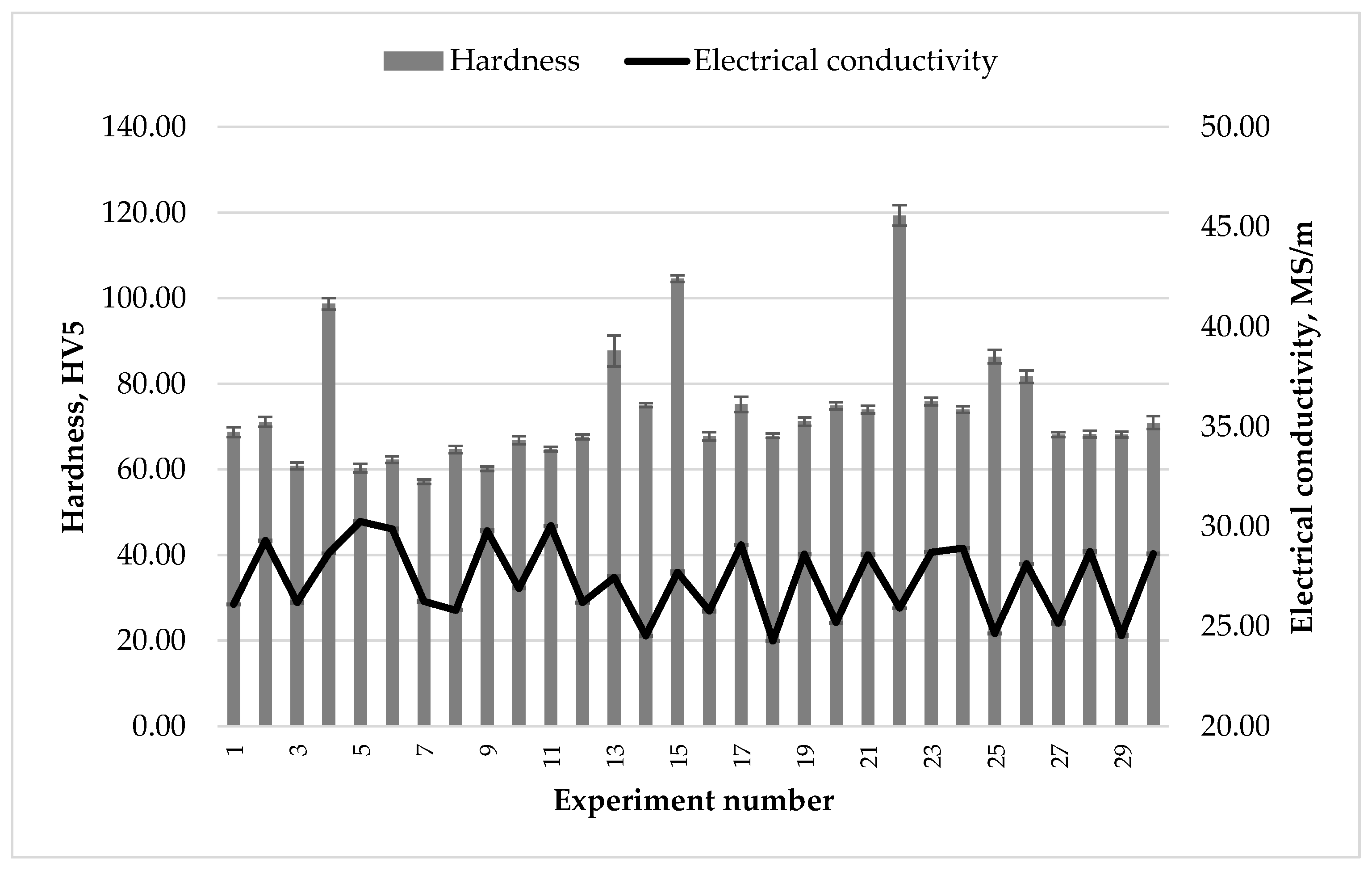
Figure 1. The mean values and standard deviations of the measured results for hardness and electrical conductivity of the flat samples.
Metals 09 00147 g001
Figure 2. The mean values and standard deviations of the measured results for tensile strength, yield strength and elongation at break of the flat samples.
Metals 09 00147 g002
Figure 3. Experimental and calculated data for the hardness and electrical conductivity. The experiment numbers are identical to the numbers in Table 3.
Metals 09 00147 g003
Table 1. Chemical analysis of the samples in wt % in comparison with the limitations of the DIN EN 573-3:2013-12.
MaterialChemical Composition in wt %
AlSiMgMnFeCuOthers
Samples alloybal.0.9160.7270.4370.3810.086<0.05
DIN EN 573-3:2013-12min.bal.0.70.60.40---
max.1.31.21.00.500.100.15
Table 2. Selected range of the heat treatment parameters and their abbreviations in the following text.
AbbreviationParametersBaseSelected Range
TsSolution temperature, °C530500–560
tsSolution time, h2.130.25–4
QMQuenching mediumWaterGas, Polymer, Water
TaAging temperature, °C170100–240
taAging time, h112–20
Table 3. Heat treatment experiments needed to create the regression model.
No.Ts (°C)ts (h)QMTa (°C)ta (h)
15000.25Water10020
25000.25Water2402
35000.25Gas1002
45000.25Gas17011
55000.25Gas24020
65000.25Polymer24020
75002.13Polymer1002
85004Water1002
95004Water24020
105004Gas10020
115004Gas2402
125004Polymer10020
135004Polymer1702
145300.25Polymer10011
155302.13Gas17020
165304Gas1002
175304Polymer2402
185600.25Water1002
195600.25Water24020
205600.25Gas10020
215600.25Gas2402
225600.25Polymer17020
235600.25Polymer24011
245602.13Polymer24011
255604Water10020
265604Water2402
275604Gas10011
285604Gas24020
295604Polymer1002
305604Polymer24020
Table 4. The significance values of the predictors.
ParametersHardnessElectrical ConductivityYield StrengthTensile StrengthElongation at Break
Constant0.0090.0001 × 10−40.0010.073
Ts0.0162 × 10−114 × 10−40.0030.005
ts0.2910.0280.1270.7840.022
QM0.0661 × 10−41 × 10−49 × 10−40.215
Ta0.0000.4570.0000.0000.879
ta3 × 10−60.0190.7711 × 10−30.155
Ts20.0190.1475 × 10−40.0040.485
ts × Ts0.2320.9750.1510.7880.021
QM × Ts0.0460.5330.2980.7850.229
Ta × Ts0.6700.3340.4180.1670.016
ta × Ts0.2130.4780.2760.3340.773
ts20.4860.0370.1200.7970.229
QM × ts0.0210.4590.3440.2060.067
Ta × ts0.4100.1790.1490.9840.294
ta × ts0.8050.7080.6130.4280.058
QM × Ta0.9230.1140.8520.2530.158
QM × ta0.1390.7140.4000.4070.301
Ta20.0000.0920.0000.0000.003
ta × Ta5 × 10−60.9655 × 10−71 × 10−40.064
ta20.1040.2310.0330.3900.011
Adj R-Square0.9520.9790.9760.9550.537
Legend:1st significance level2nd significance level3rd significance level4th significance levelout of the model