Welding Window: Comparison of Deribas’ and Wittman’s Approaches and SPH Simulation Results

Abstract

A welding window is one of the key concepts used to select optimal regimes for high-velocity impact welding. In a number of recent studies, the method of smoothed particle hydrodynamics (SPH) was used to find the welding window. In this paper, an attempt is made to compare the results of SPH simulation and classical approaches to find the boundaries of a welding window. The experimental data on the welding of 6061-T6 alloy obtained by Wittman were used to verify the simulation results. Numerical simulation of high-velocity impact accompanied by deformation and heating was carried out by the SPH method in Ansys Autodyn software. To analyze the cooling process, the heat equation was solved using the finite difference method. Numerical simulation reproduced most of the explosion welding phenomena, in particular, the formation of waves, vortices, and jets. The left, right, and lower boundaries found using numerical simulations were in good agreement with those found using Wittman’s and Deribas’s approaches. At the same time, significant differences were found in the position of the upper limit. The results of this study improve understanding of the mechanism of joint formation during high-velocity impact welding.

1. Introduction

High-velocity impact welding is one of the best methods for joining dissimilar materials. This group of welding processes include explosive welding, magnetic pulse welding, laser impact welding, etc. Among multiple parameters of these processes, the collision point velocity ($V_c$) and the collision angle ($\alpha$) are of the highest importance to select the regime of welding. Thus, the choice of the welding regime, as a rule, is associated with establishing the optimal combination of these two values. For most materials, the range of $V_c$ and $\alpha$ is quite wide, so in the diagrams plotted in the coordinates ($V_c$–$\alpha$), a large range of regimes providing reasonable welding quality can be distinguished. This area is called the welding window (or weldability window). An example of weldability window is shown in Figure 1.

Among the pioneering studies in which successful attempts were made to determine the boundaries of the weldability window, it is worth highlighting the studies of Wittman [1] and Deribas [2]. Their approaches are still widely used in practice to select welding regimes. The approaches to determining the lower and right boundaries used by both authors almost coincide. However, the position of the upper limit calculated according to the formulas stated in their studies differs (as a rule, the Deribas calculation predicts a wider range of acceptable welding regimes). Despite the fact that in many cases the classical approaches to constructing a weldability window work quite well, their application is difficult when working with dissimilar materials. In addition, adequately describing the boundaries of the weldability window, the expressions used do not give an idea of the mechanics of the deformation process near the interlayer boundary and practically do not discuss the formation of melt zones in explosively welded joints.

To address these issues, in recent studies [3,4,5,6] the weldability window was found using smoothed particle hydrodynamics (SPH) simulation. SPH technique was used extensively in recent years to analyze various aspects of high-velocity impact welding. Unlike other methods, for example, Euler or Lagrangian, SPH reproduces well the basic phenomena associated with high-velocity impact welding-the formation of jets, waves and vortex zones, and it is well suited for analyzing the pressures in the impact zone [4,7,8,9,10,11,12,13,14].

This study compares approaches to constructing a weldability window proposed by Deribas and Wittman with an approach based on SPH simulation. Aluminum alloy 6061-T6 was used as a material for analysis. A large amount of experimental data on explosive welding of this alloy presented by Wittman [1] was used to verify the simulation results. In this study, an attempt was made to determine the regimes of formation and disappearance of a jet, the area of wave formation and vortex zones using numerical simulation and “classical” approaches proposed by Deribas and Wittman. To assess the upper limit of the weldability window, the influence of melt zones and their cooling rates on the formation of joints was analyzed. In addition, the paper discusses the features of the plastic flow of material near the interface, which are compared with experimental data obtained in the works of Chugunov et al. [15].

The majority of recent studies devoted to numerical simulation of high-velocity impact welding consider only few collision regimes providing only a limited understanding of the bonding phenomena [16,17,18]. Besides, most of the currently existing SPH studies on high-velocity impact welding simply state the fact of good agreement between the simulation results and experimentally observed interface. The relationship between the flow of individual particles and the jetting and wave formation is usually not discussed. Thus, the understanding of some important phenomena is still limited. In the current study, we simulated a large number of welding regimes, varying the collision angle and collision velocity. Thus, a more complete understanding of the bonding phenomena was achieved.

From the practical point of view, this study is interesting for engineers, who are responsible for selection of regimes of high-velocity impact welding as it provides better understanding of the weldability window concept. The application of SPH simulation will allow to predict the shape of the interface and minimize the amount of liquid phase which may appear when the collision velocity is too high. Understanding of the thermal situation near the interface allows predicting the phases which may appear due to the high cooling rates.

2. Description of Numerical Simulation

2.1. Simulation of Impact

Plates of 6061-T6 aluminum alloy with dimensions of 63.5 × 6 mm² were used for numerical simulation. This material was chosen due to the previous study of Wittman [1], who published a significant amount of experimental data on explosive welding of this alloy and described the morphology of the interlayer boundaries and the properties of the joints. Thus, the data obtained by Wittman were used for comparison with data obtained by simulation.

The computational domain is shown in Figure 2. At the initial moment of time, the flyer plate had a velocity $V_p$ and it was positioned at an angle $\alpha$ with respect to the base plate. The collision point velocity ($V_c$) was determined in accordance with the Equation [1]:

$$V_p=2V_c\sin \frac{\alpha }{2}$$

(1)

In this study, a series of simulations were carried out in which the angle varied from 5° to 40° with a step of 5°, and the collision point velocity varied from 500 m/s to 9300 m/s with a step of 800 m/s. After the approximate position of the lower limit was found, a series of additional simulations were carried out in order to specify the minimum welding parameters with greater accuracy.

The collision process was simulated in the Ansys Autodyn 19 software using the SPH method. This method is well suited for simulating phenomena associated with large strains and rapidly moving borders. In a number of previous studies, this method was successfully used to simulate high-velocity impact welding of similar [4,19,20,21] as well as dissimilar materials [17,22,23,24] showing a very good agreement between the simulation results and experiments.

High-velocity impact can lead to the formation of shock waves in the material. At a shock wave-front, discontinuity in materials properties is observed. For numerical analysis of discontinuity, it is required to set the properties before and after the shock front. For this reason, the modified Mie-Grüneisen equation of state based on the Hugoniot shock adiabat was used [25]:

$$p=p_H+\Gamma \rho \left(e-e_H\right),$$

(2)

where $p$ is the pressure, $p_H$ is the Hugoniot pressure, Γ is the Grüneisen gamma, $e$ is the internal energy, $e_H$ is the Hugoniot internal energy. For solid materials, the equation of the Hugoniot shock adiabat can be written in the following form:

$$U_s=C_1+S_1{U}_P,$$

(3)

where $U_s$ is the shock velocity, $U_P$ is the particle velocity, $C_1$, $S_1$ are empirically determined coefficients depending on the material.

The coefficients used in this study are shown in

Table 1. Parameters of the modified Mie-Grüneisen equation of state for aluminum alloy 6061-T6.

Parameter	Value	Units
Reference density	2.7	g/cm3
Grüneisen parameter	1.97	-
Parameter $C_1$	5.35	m/ms
Parameter $S_1$	1.34	-
Reference Temperature	293	K
Specific Heat	8.85·10−4	kJ/(g·K)

.

The dependence of the material’s strength on the deformation conditions was taken into account by using the Johnson-Cook empirical model, which is widely used in the simulation of various phenomena associated with a high-velocity deformation [26,27]. This model allows considering the influence of strain hardening, thermal softening, and a strain rate on the yield stress of the material and it is described by the following Equation:

$$\sigma =\left(A+B{\epsilon }^n\right)\left(1+C\ln {\dot{\epsilon }}^{*}\right)\left(1-T^{{*}^m}\right),$$

(4)

where $\sigma$ is the current yield strain, $\epsilon$ is the effective plastic strain, $\dot{\epsilon }$* is the dimensionless plastic strain rate, $T^{*}=\frac{T-T_r}{T_m-T_r}$, $T$ is the current temperature, $T_m$ is the melting temperature, $T_r$ is the reference temperature. $A$, $B$, $C$, $n$ and $m$ are the material constants determined from an empirical fit of flow stress data, $A$, $B$ and $n$ are the yield stress, the hardening constant and the hardening exponent associated with quasi-static test respectively, $C$ is the strain rate constant, $m$ is the thermal softening exponent. The constants used in the Johnson-Cook model for Al 6061-T6 are shown in

Table 2. Johnson-Cook model parameters [28,29].

Parameter	Value	Units
Shear Modulus	26	GPa
Yield Stress	0.324	GPa
Hardening Constant	0.114	GPa
Hardening Exponent	0.42	-
Strain Rate Constant	0.002	-
Thermal Softening Exponent	1.34	-
Melting Temperature	925	K
Ref. Strain Rate (/s)	1	-

.

2.2. Description of Cooling Model

The estimation of time which material spent in the molten state is of fundamental importance to assess the upper limit of welding. It is believed that, if this time is less than the duration of compressive stresses, a joint will form. Otherwise, the incoming tensile wave breaks the joint that did not have enough time to solidify. It should be noted that the system of equations used by Autodyn software does not consider the heat transfer. Therefore, it is believed that the deformation process is completely adiabatic. For this reason, the calculation of the cooling process was carried out separately using self-developed code in Python programming language. The temperatures obtained by simulation in Autodyn were exported as a text file and were used as initial conditions for solving the heat equation, which in the 2D case can be written as follows:

$$\frac{\partial U}{\partial t}=ɑ\left(\frac{{\partial }^{2}U}{\partial x^2}+\frac{{\partial }^{2}U}{\partial y^2}\right),$$

(5)

where $U=\left(x, y, t\right)$ is the function that describes the temperature at a point with $x$ and $y$ coordinates at the moment of time $t$, $ɑ$ is the thermal diffusivity.

The equation was solved by the finite difference method in a “Forward-Time Central-Space” explicit scheme. In this case, it was believed that the outer boundaries of the plates were isolated from the environment, and cooling occurred due to heat transfer from the interface to the inner volumes of the plates, which practically did not heat up during a collision.

3. Results and Discussion

Figure 3a shows the results of an experimental study of 6061-T6 alloy explosive welding performed by Wittman. Based on these studies, he developed approaches to calculate the limiting conditions that provided a satisfactory quality of the joint and built a weldability window also plotted in Figure 3a. For the upper limit of the weldability window shown in Figure 3a, two lines are plotted: one of them is based on the predictions of Wittman’s model, and the other is based on the estimations of Deribas [30]. Figure 3b represents the simulation results showing the regions of modes characterized by the absence of a jet, the presence of a jet, and the simultaneous presence of a jet and waves at the interface. In addition, the limits of welding calculated based on approaches of Deribas and Wittman are also plotted in this Figure for comparison purpose. In the following sections of the paper, each of these limits is discussed in detail.

3.1. The Lower Limit of the Weldability Window

The lower limit of the weldability window represents the locus of points that define the “softest” welding regimes, below which the collision does not lead to the formation of a strong bond. Following the reasoning typical for various solid-state welding methods, the impact should ensure the achievement of a certain critical degree of plastic strain and cooperative flow of the impacted plates, providing activation of the welded surfaces.

One of the conditions necessary for the joint formation in the process of high-velocity collision is considered to be the jet formation in front of the contact point [1,2,30]. This jet consists of the material of the surface layers of the impacted plates, which is ejected from the welding zone in the form of a peculiar cloud [4] providing contact to surfaces free from contamination. Deribas called this phenomenon self-cleaning [2]. In their studies, Deribas and Wittman believed that the critical regimes of jet formation determine the lower limit of the weldability window in the subsonic range. At the same time, both researchers developed an entirely empirical criterion which suggests that the pressure in the collision zone should be several times higher than the Hugoniot elastic limit (5 times according to Wittman [1]). In the same time, the study [1] does not give clear explanations for the choice of the empirical coefficient. It can be assumed that this coefficient was chosen to fit the calculated position of the lower boundary as closely as possible to the experimental data. In the absence of data on the Hugoniot elastic limit, the critical impact velocity that ensures jet formation according to Wittman can also be found using the following empirical expression:

$$V_p=\sqrt{\frac{{\sigma }_{ts}}{{\rho }_f}},$$

(6)

where ${\sigma }_{ts}$ is the tensile strength and ${\rho }_f$ is the material density.

This expression was used to plot the line A in Figure 3a.

It can be noted that jet formation was observed for most collision regimes analyzed by numerical simulation (Figure 3b). The lower limit predicted by the calculation has a similar trend to the line A, however, it is located more to the upper right part of the diagram, which may be due to the insufficient spatial resolution to simulate weak jets at relatively soft collision regimes.

To understand the reasons leading to the formation of a jet, it is interesting to analyze the differences in conditions near the contact point for some regimes between $V_c$ = 1300 m/s and $V_c$ = 9300 m/s at a constant collision angle $\alpha$ = 15° (Figure 4a–e). The collision point velocity equal to $V_c$ = 1300 m/s corresponds to the regime at which the jet is not formed yet (Figure 4a), while collision point velocity of $V_c$ = 1700 m/s provides the first signs of the weak jet formation (Figure 4b). At higher collision point velocities (Figure 4c–e), the jet becomes more noticeable until it finally disappears when crossing the so-called supersonic limit of the weldability window (Figure 4f), which occurs for the reasons described in the next section. One can observe the specific nature of the pressure distribution near the collision point in the modes corresponding to the jet formation. The pressure distribution lines are convex in the direction of collision point movement and at the same time, high pressures outpace it to some extent. This shape of the pressure distribution zone causes the surface layer material to rise above the surface forming an elevation when approaching the collision point. Thus, the collision angle of the plates in the immediate vicinity of the collision point increases compared to the initial collision angle $\alpha$. Further, the material of the surface layers “flies” onto the area of extremely high pressures and is thrown forward in the form of a peculiar jet. It should be noted that the term “jet” as applied to explosive welding should be used cautiously. Experiments carried out in a number of studies indicate that due to the heating, the material moving in front of the collision point represents a cloud (probably a plasma cloud) rather than a liquid metal [2,4,32].

From the current simulation, it follows that Wittman′s assumption that the pressure near the collision point should substantially exceed the strength of the material for the jet to form seems plausible. Taking into account the deformation conditions typical for the high-velocity impact welding (strain, strain rate and temperature), and inserting them in Equation (4) it can be found that the yield strength of 6061-T6 alloy can reach 0.45 GPa. In the current simulation, a weak jet was formed when the pressure near the collision point was approximately 2 GPa or more (that was about 5 times higher than the yield strength estimated by Equation (4)) (Figure 4b), and a stable jet could be formed when the pressure at the collision point exceeded 4 GPa (Figure 4c). Weaker pressures did not lead to the formation of a significant elevation and the material of the surface layer “entered” the collision point at an acuter angle. Moreover, according to the simulation, the strain near the interface exceeded $\epsilon$ = 1.5 for the regimes corresponding to the jet formation (for the regimes near the lower limit) and could be significantly larger for the regimes located near the right limit of the weldability window.

3.2. Supersonic Limit

At extremely high collision velocities, a jet does not form, and the surface self-cleaning phenomenon is not observed. In addition, tensile waves quickly come into the deformed area, which does not give sufficient time for solidification and leads to the destruction of the joint. In many studies (for instance, [33,34,35]), little attention is paid to the right limit of welding when constructing a weldability window. It is common to simplify its position by taking the maximum allowed collision velocity equal to the bulk sound velocity of welded materials. Although from a practical point of view this simplification is probably acceptable, since welding at such high velocities is quite rare, nevertheless, these simplifications do not correspond to real experiments. The concept of the critical angle for jet formation at supersonic velocities was considered in detail in the studies of Walsh et al. [11] and Cowan et al. [19], and an example of its practical application was considered in detail in [36]. According to this concept, at high collision point velocity, a jet is formed only if the collision angle exceeds a certain threshold value. In pursuance of the instructions given in [36,37,38,39], the following set of equations was obtained:

$$\tan \alpha =\frac{\left(\left(\sin \beta -5.35/V_c\right)/1.34\right)\sqrt{1-{\sin }^2\beta }}{\left(1-\sin \beta \left(\sin \beta -5.35/V_c\right)/1.34\right)},$$

(7)

$$p=\rho \left(V_c\sin \beta \right)\left(V_c\sin \beta -5.35\right)/1.34,$$

(8)

$$U_S=5.35+1.34U_P,$$

(9)

$$U_S=V_c\sin \beta ,$$

(10)

where $\beta$ is the angle between the shock front and the vector of material flow into the collision point.

By varying $\beta$ in the range from 0 to 90°, it is possible to develop a set of plots of $\beta$ versus $p$ for each $V_c$ value. The obtained curves with a specific maximum provide the value of the critical angle of jet formation $\alpha$ for a given collision point velocity $V_c$ (line B in Figure 3a).

One can note that there is a very good agreement between the position of the right limit, which was determined in accordance with [37,38] and in accordance with the results of SPH simulation (Figure 3b). With an increase of collision point velocity, the pressure front was getting more and more straightened (Figure 4f). Thus, the specific elevation of the surface layers in front of the contact point described in the previous section was barely observed and the plates collided at an acute angle without jet formation.

3.3. Wave Formation Limit

The wave formation at the interface is one of the features typical for high-velocity impact welding. However, it should be noted that a number of studies [40,41,42,43] showed that the mechanical properties of joints with a flat interface were as high as those with wavy ones. For this reason, the process of wave formation is primarily of fundamental interest. However, it is likely that a complete understanding of the explosive welding process is impossible without understanding the wave formation process.

One of the first sufficiently reliable criteria for the wave formation was proposed by Cowan et al. [8], who came to the conclusion that the transition from waveless to wavy mode of welding depends only on the collision point velocity. They found $\mathrm{that}$ for each combination of materials there is such a critical collision point velocity ($V_T)$, above which the wave formation occurs, and they proposed the following Equation:

$$V_T= \sqrt{2R_T\left(H_f+H_b\right)/\left({\rho }_f+{\rho }_b\right)},$$

(11)

where ${\rho }_f$ and ${\rho }_b$ are the densities of flyer and base plates, respectively, $H_f$ and $H_b$ are the diamond pyramid hardness of flyer and base plates, respectively. R_T is an empirically determined parameter, introduced by analogy with the Reynolds number. The critical value of $R_T$ leading to the wave formation varies in the range from 8.1 to 13.1 for different materials, which was established experimentally in [44]. This expression was used to construct line C in Figure 3a. In this case, following the data presented in [44], the value $R_T=8$ was used to plot the line C.

It can be seen in Figure 3 that the critical value of the collision point velocity calculated using Equation (11), which describes the transition to wave formation, is in a good agreement with the results of Wittman′s experimental studies. However, it should be noted that several studies showed that the transition to wave formation depends both on the collision point velocity and on the collision angle (for example, Szecket [45], or Lysak and Kuzmin [46]). This assumption is also supported by the results of the current numerical simulation (Figure 3b). One can note that at large collision angles, wave formation began at lower velocities than at small angles. Thus, the shape of the wave transition limit resembles line A more than line C, i.e., the transition to wave formation occurred at a certain critical flyer plate velocity, and not at some constant collision point velocity.

It is interesting to note that for regimes with very high $V_c$ located slightly to the left of the jet formation limit, the wave formation terminated again. Thus, it can be assumed that there are two boundaries of wave formation-left and right. In principle, the termination of the wave formation process at high collision point velocities is described in a number of experimental works (e.g., [47,48]), however, the reasons of this phenomenon require additional study.

One can note a good agreement between the nature of material flow predicted by simulation and observed in experimental studies. For example, Figure 5a shows the deformation of the experimental grid after explosive welding of aluminum alloy plates. This image was obtained in the experiments of Chugunov et al. [15] using laminated inserts made of the material similar to the material of welded plates. The laminated nature of the inserts was used to track the peculiarities of plastic deformation near the interface. In Figure 5b an attempt to reproduce this experiment using SPH simulation is shown. To do this, the particles forming a square mesh were marked before the simulation was started. During the simulation, the positions of these particles were tracked, and the deformation of the mesh was observed. As it is seen from Figure 5, the flow pattern of the material observed in the simulation was in good agreement with that observed in the experiments. As an example, the flow patterns for different collision regimes are shown in Figure 6. It can be noted that the plastic strain substantially increased closer to the interface. Moreover, with an increase in the collision point velocity, the plastic strain also increased significantly. The proposed approach allows one to visualize the features of material deformation during explosion welding. In particular, it can be noted that the deformation of mesh cells in the flyer and base plates is different, which is probably due to the asymmetry of the collision scheme.

3.4. Upper Limit

The upper limit of the weldability window attracted much less attention of researchers than the lower one and the issues of transition from waveless to wavy modes of welding. This is probably due to the fact that the welding regimes near the lower limit are more preferable for industrial applications. However, the position of the upper limit is important from both industrial and fundamental points of view. It should be noted that welding using the regimes near the upper limit of the weldability window may lead to the formation of an excessive amount of molten zones leading to embrittlement of the welded joint and decrease in its strength.

So far, there are two main studies devoted to the analysis of the upper limit of the weldability window known from the literature—the study of Wittman [1] and the study of Efremov and Zakharenko [31]. The later became known due to the monographs of Deribas [2] and Zakharenko [49]. A common feature of both approaches is the comparison of the compressive stresses’ duration in the deformed area with the time required to cool the material.

In his study, Wittman came to the following expression, limiting the highest allowable flyer plate velocity $V_{max}$:

$$V_{max}={\left(T_m{C}_B\right)}^{1/2}{\left(ɑc{C}_B\right)}^{1/4}/N{V}_c{\left(\rho h_f\right)}^{1/4},$$

(12)

where $T_m$ is the material melting temperature, $C_B$ is the bulk sound velocity, $c$ is the specific heat, $h_f$ is the flyer plate thickness, $N$ is empirically determined material-dependent coefficient. In the case of Al6061-T6 aluminum, alloy $N$ is equal to 0.11. It should be also noted that all Wittman’s calculations were performed in the CGS units, so when calculating in SI units the value of the coefficient $N$ will be different.

In the work of Efremov and Zakharenko, the following equation was proposed, limiting the highest collision angle as a function of the collision point velocity and the thermophysical material properties:

$$\sin \frac{\alpha }{2}=11.8\ast V_c^{-5/4}\sqrt{\frac{T_m\frac{\chi }{ɑ}}{\rho \frac{h_b}{h_f+h_b}\sqrt{h_f}}}\sqrt[4]{\xi },$$

(13)

where $\chi$ is the thermal conductivity, $h_b$ is the thickness of the base plate, $\xi = x^{*}/h_f$, $x^{*}$ is the distance from the collision point to the point behind it where the tensile stresses are achieved. To simplify the calculations, it is common to consider that $\sqrt[4]{\xi }$ = 1. The empirical coefficient equal to 11.8, which characterizes the amount of heat released and the irregularity of the melt location along the interface, was selected in [50] so that the calculated upper limit provides the best fit to the data obtained in practical studies. In the paper [51], it is proposed to use the coefficient 14.7 instead.

From Figure 3 it can be noted that Equation (12) gives a lower critical impact velocity, and, accordingly, a narrower weldability window, as compared to Equation (13).

To calculate the position of the upper limit using numerical simulation, it is reasonable to follow the same sequence of reasoning—firstly, it is necessary to calculate the duration of compressive stresses, and then compare the calculated time with that required to cool the weld below the melting temperature.

Typical pressure history in a point located near the interface is shown in Figure 7. It is possible to determine the time available for the material to cool, by measuring the time from the moment when the peak pressure is reached until the moment when the tensile wave arrived.

The duration of compressive stresses on the collision regimes is shown in Figure 8. To determine the average value and the confidence interval, five measurements were carried out at various points along the interface. It can be noted that in the presented range of collision angles, the collision point velocity had the greatest impact on this parameter.

Figure 9 shows a typical calculation of the cooling process in the vicinity of the contact point for $V_c$ = 2100 m/s and $\alpha$ = 20°. The information about the temperature distribution obtained using SPH simulation in Ansys Autodyn was used as initial conditions for the heat equation. It should be noted that the time required for complete solidification of the material in the region of the interface exceeded the lifetime of compressive stresses in the weld. As already noted, the micro-volumes of the liquid phase were distributed unevenly along the weld, forming vortex zones on the sides of the waves. This process is explained by redistribution of the liquid phase behind the collision point in the process of wave growth, as it was previously shown in [4]. The current simulation shows, that these micro-volumes can remain in a partially molten state at the time of the arrival of the tensile wave. Due to this reason, they can’t provide strong bonding and withstand tensile stresses. Thus, the bonding of the material near the upper limit entirely depends on the areas of interface free of liquid phase, where the direct contact of solid materials is possible, or on the areas where the liquid phase volume is extremely small. These areas allow the joint to withstand the passage of the tensile wave, while the final solidification of the melt clumps (i.e., vortex zones) probably occurs later.

According to Figure 10, the volume of molten metal at the interface raises almost linearly with the collision point velocity increase, and also, as a rule, slightly increases with an increase in the collision angle. Considering that the position of the upper welding limit described by Wittman is the most accurate (since it was received from the experiment), it is interesting to estimate the amount of the liquid phase near the interface defined by line D in Figure 3a. It can be noted that for all collision regimes close to line D, the liquid phase volume fraction was at the level of about 1% of the total plate volume. According to Efremov and Zakharenko (line D ’in Figure 3a), for the regimes located near the upper limit the estimated volume fraction of the liquid phase was at the level of 4–6%. It should be noted that determining the upper limit of the welding window, Wittman believed that the joint above this limit would have insufficient mechanical properties, while in Deribas′s work it was supposed that the welding of the plates outside the upper limit would not occur in principle, since a tensile wave will lead to the destruction of the non-solidified weld joint. Thus, for the formation of a high-quality joint, the volume fraction of the liquid phase probably should not significantly exceed 1%. Nevertheless, this criterion requires more thorough experimental verification for materials of other compositions and other thicknesses.

From the simulation, it follows that the volume fraction of molten metal is always slightly higher for a base plate, and the difference becomes more noticeable for high welding velocities (Figure 11).

4. Conclusions

Based on the results of numerical simulation and their comparison with experimental data of Wittman, we can draw the following conclusions:

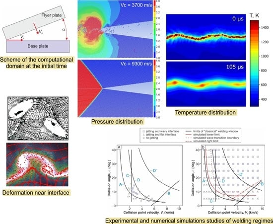
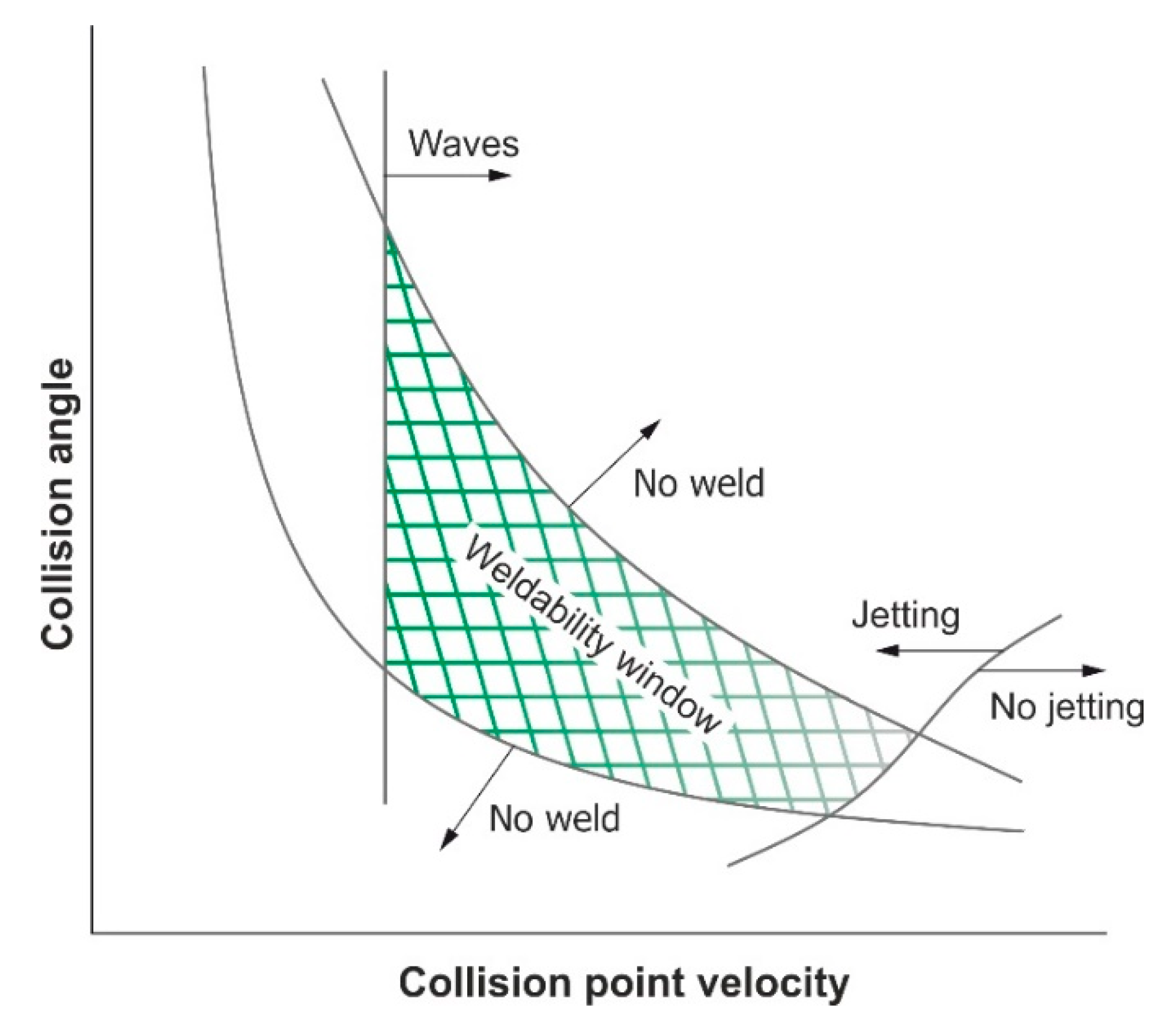
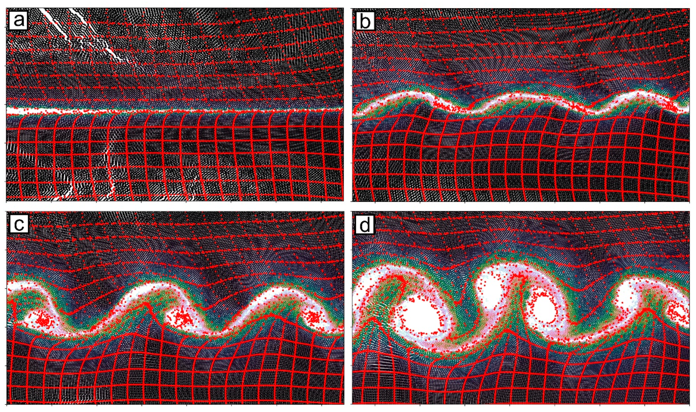
• SPH simulation reproduces all the basic phenomena typical for the high-velocity impact welding process: the jet (or cloud) formation in front of the collision point, the wave formation, as well as the material deformation mechanism near the interface. Flow patterns near the interface are in good agreement with the results of experimental studies obtained by other authors. The proposed approach allows one to build the weldability windows.
• The simulated lower welding limit slightly differs from the results of Wittman′s theoretical and experimental studies. While Wittman observed bonding (which implies the existence of a jet) even at very low collision angles (around 5 degrees), the simulation predicts jetting when the collision angle exceeds 7.5 or even 10 degrees. This may be due to inaccuracies in the material models used in the current simulation, as well as due to the insufficient resolution for observing weak jets.
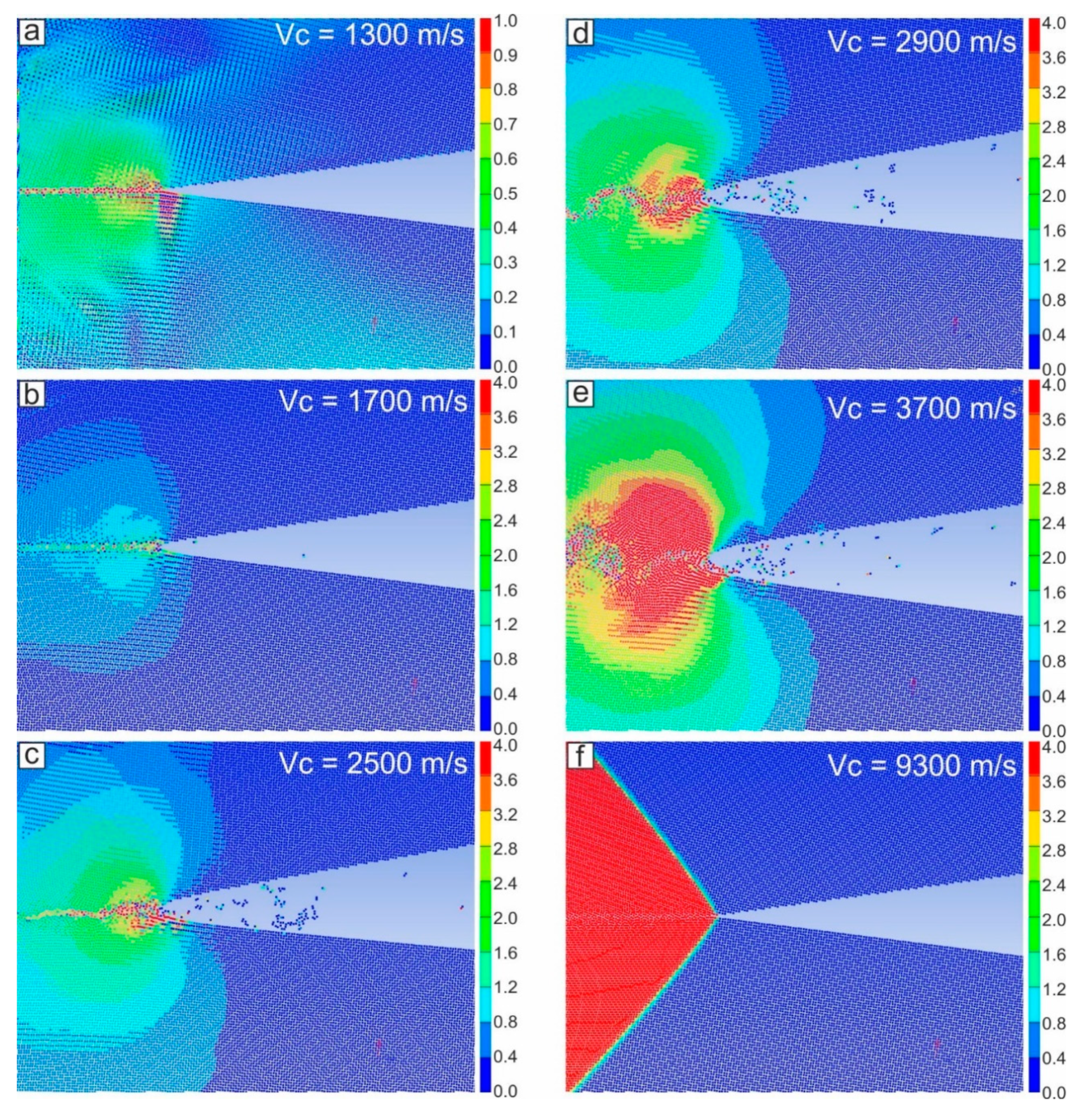
• The wave formation starts when the collision point velocity exceeds 1700 m/s. However, in comparison with most of the previous studies, the wave transition velocity turned out to be dependent on the collision angle. At low collision angles (e.g., 10 degrees), the transition to the wavy interface occurred around 4000 m/s.
• The numerical simulation predicts the existence of the right limit of wave formation, which is consistent with several experimental studies. The transition to straight interface coincides with the supersonic limit of welding.
• The position of the upper limit of the weldability window is difficult to determine using the model considered in the current study. The lifetime of compressive stresses is shorter than the time required for complete solidification of the molten areas. Thus, the joint formation near the upper limit is most likely occurs due to the presence of areas where direct contact in the solid phase is formed. Further refinement of the position of the upper limit requires the simultaneous solution of heat and deformation problems and is of interest for further studies. However, from a practical point of view, the welding regimes used in the industry should be closer to the lower limit of the weldability window. Thus, this approach can be used in practice.

References

1. Wittman, R.H. The influence of collision parameters of the strength and microstructure of an explosion welded aluminium alloy. In Proceedings of the Proc. 2nd Int. Sym. on Use of an Explosive Energy in Manufacturing Metallic Materials, Marianske Lazne, Czech Republic, 9–12 October 1973; pp. 153–168. [Google Scholar]
2. Deribas, A.A. Физика упрочнения и сварки взрывом; Nauka: Novosibirsk, Russia, 1980. [Google Scholar]
3. Zhang, Z.L.; Ma, T.; Liu, M.B.; Feng, D. Numerical Study on High Velocity Impact Welding Using a Modified SPH Method. Int. J. Comput. Methods 2019, 16, 1–24. [Google Scholar] [CrossRef]
4. Bataev, I.A.; Tanaka, S.; Zhou, Q.; Lazurenko, D.V.; Junior, A.M.J.; Bataev, A.A.; Hokamoto, K.; Mori, A.; Chen, P. Towards better understanding of explosive welding by combination of numerical simulation and experimental study. Mater. Des. 2019, 169, 107649. [Google Scholar] [CrossRef]
5. Zhang, Z.L.; Liu, M.B. Numerical studies on explosive welding with ANFO by using a density adaptive SPH method. J. Manuf. Process. 2019, 41, 208–220. [Google Scholar] [CrossRef]
6. Zhang, Z.L.; Feng, D.L.; Liu, M.B. Investigation of explosive welding through whole process modeling using a density adaptive SPH method. J. Manuf. Process. 2018, 35, 169–189. [Google Scholar] [CrossRef]
7. Bataev, I. Structure of Explosively Welded Materials: Experimental Study and Numerical Simulation. Met. Work. Mater. Sci. 2017, 4, 55–67. [Google Scholar] [CrossRef]
8. Feng, J.; Chen, P.; Zhou, Q.; Dai, K.; An, E.; Yuan, Y. Numerical simulation of explosive welding using Smoothed Particle Hydrodynamics method. Int. J. Multiphys. 2017, 11, 315–325. [Google Scholar]
9. Nassiri, A.; Chini, G.; Vivek, A.; Daehn, G.; Kinsey, B. Arbitrary Lagrangian-Eulerian finite element simulation and experimental investigation of wavy interfacial morphology during high velocity impact welding. Mater. Des. 2015, 88, 345–358. [Google Scholar] [CrossRef]
10. Vivek, A.; Liu, B.C.; Hansen, S.R.; Daehn, G.S. Accessing collision welding process window for titanium/copper welds with vaporizing foil actuators and grooved targets. J. Mater. Process. Technol. 2014, 214, 1583–1589. [Google Scholar] [CrossRef]
11. Liu, C.B.; Palazotto, A.N.; Nassiri, A.; Vivek, A.; Daehn, G.S. Experimental and numerical investigation of interfacial microstructure in fully age-hardened 15-5 PH stainless steel during impact welding. J. Mater. Sci. 2019, 54, 9824–9842. [Google Scholar] [CrossRef]
12. Lee, T.; Zhang, S.; Vivek, A.; Daehn, G.; Kinsey, B. Wave formation in impact welding: Study of the Cu–Ti system. CIRP Ann. 2019, 68, 261–264. [Google Scholar] [CrossRef]
13. Nassiri, A.; Vivek, A.; Abke, T.; Liu, B.; Lee, T.; Daehn, G. Depiction of interfacial morphology in impact welded Ti/Cu bimetallic systems using smoothed particle hydrodynamics. Appl. Phys. Lett. 2017, 110, 231601. [Google Scholar] [CrossRef]
14. Nassiri, A.; Zhang, S.; Lee, T.; Abke, T.; Vivek, A.; Kinsey, B.; Daehn, G. Numerical investigation of CP-Ti and Cu110 impact welding using smoothed particle hydrodynamics and arbitrary Lagrangian-Eulerian methods. J. Manuf. Process. 2017, 28, 558–564. [Google Scholar] [CrossRef]
15. Chugunov, E.A.; Kuzmin, S.V.; Lysak, V.I.; Peev, A.P. Основные закономерности деформирования металла околошовной зоны при сварке взрывом алюминия. Phys. Chem. Mater. Treat. 2001, 3, 39–44. [Google Scholar]
16. Mahmood, Y.; Dai, K.; Chen, P.; Zhou, Q.; Bhatti, A.A.; Arab, A. Experimental and Numerical Study on Microstructure and Mechanical Properties of Ti-6Al-4V/Al-1060 Explosive Welding. Metals 2019, 9, 1189. [Google Scholar] [CrossRef] [Green Version]
17. Li, Y.; Liu, C.; Yu, H.; Zhao, F.; Wu, Z. Numerical simulation of Ti/Al bimetal composite fabricated by explosive welding. Metals 2017, 7, 407. [Google Scholar] [CrossRef] [Green Version]
18. Wang, X.; Zheng, Y.; Liu, H.; Shen, Z.; Hu, Y.; Li, W.; Gao, Y.; Guo, C. Numerical study of the mechanism of explosive/impact welding using Smoothed Particle Hydrodynamics method. Mater. Des. 2012, 35, 210–219. [Google Scholar] [CrossRef]
19. Nassiri, A.; Kinsey, B. Numerical studies on high-velocity impact welding: Smoothed particle hydrodynamics (SPH) and arbitrary Lagrangian–Eulerian (ALE). J. Manuf. Process. 2016, 24, 376–381. [Google Scholar] [CrossRef] [Green Version]
20. Liu, M.B.; Zhang, Z.L.; Feng, D.L. A density-adaptive SPH method with kernel gradient correction for modeling explosive welding. Comput. Mech. 2017, 60, 513–529. [Google Scholar] [CrossRef]
21. Tanaka, K. Numerical studies on the explosive welding by smoothed particle hydrodynamics (SPH). AIP Conf. Proc. 2007, 955, 1301–1304. [Google Scholar]
22. Zhou, Q.; Feng, J.; Chen, P. Numerical and experimental studies on the explosive welding of tungsten foil to copper. Materials 2017, 10, 984. [Google Scholar] [CrossRef]
23. Nishiwaki, J.; Sawa, Y.; Harada, Y.; Kumai, S. SPH analysis on formation manner of wavy joint interface in impact welded Al/Cu dissimilar metal plates. Mater. Sci. Forum 2014, 794–796, 383–388. [Google Scholar] [CrossRef]
24. Chu, Q.; Zhang, M.; Li, J.; Yan, C. Experimental and numerical investigation of microstructure and mechanical behavior of titanium/steel interfaces prepared by explosive welding. Mater. Sci. Eng. A 2017, 689, 323–331. [Google Scholar] [CrossRef]
25. Meyers, M.A. Dynamic Behavior of Materials; John Wiley & Sons, Inc.: Hoboken, NJ, USA, 1994; ISBN 9780470172278. [Google Scholar]
26. Johnson, G.R.; Cook, W.H. A constitutive model and data for metals subjected to large strains, high strain rates and high temperatures. In Proceedings of the 7th International Symposium on Ballistics, the Hague, The Netherlands, 19–21 April 1983; pp. 541–547. [Google Scholar]
27. Johnson, G.R.; Cook, W.H. Fracture characteristics of three metals subjected to various strains, strain rates, temperatures and pressures. Eng. Fract. Mech. 1985, 21, 31–48. [Google Scholar] [CrossRef]
28. Corbett, B.M. Numerical simulations of target hole diameters for hypervelocity impacts into elevated and room temperature bumpers. Int. J. Impact Eng. 2006, 33, 431–440. [Google Scholar] [CrossRef]
29. Lesuer, D.R.; Kay, G.J.; LeBlanc, M.M. Modeling Large-Strain, High-Rate Deformation in Metals. In Proceedings of the Third Biennial Tri-Laboratory Engineering Conference Modeling and Simulation, Pleasanton, CA, USA, 3–5 November 1999. [Google Scholar]
30. Deribas, A.A. Classification of flows appearing on oblique collisions on metallic plates. In Proceedings of the Proc. 2nd Int. Sym. on Use of an Explosive Energy in Manufacturing Metallic Materials, Marianske Lazne, Czech Republic, 9–12 October 1973; pp. 31–44. [Google Scholar]
31. Efremov, V.V.; Zakharenko, I.D. Determination of the upper limit to explosive welding. Combust. Explos. Shock Waves 1977, 12, 226–230. [Google Scholar] [CrossRef]
32. Mali, V.I.; Simonov, V.A. Some effects appearing on interactions of shock waves with cavities in metals. In Proceedings of the Proc. 2nd Int. Sym. on Use of an Explosive Energy in Manufacturing Metallic Materials, Marianske Lazne, Czech Republic, 1974; pp. 83–96. [Google Scholar]
33. Carvalho, G.H.S.F.L.; Galvão, I.; Mendes, R.; Leal, R.M.; Loureiro, A. Explosive welding of aluminium to stainless steel. J. Mater. Process. Technol. 2018, 262, 340–349. [Google Scholar] [CrossRef]
34. Wu, Y.; Lu, J.; Tan, S.; Jiang, F.; Sun, J. Modified implementation strategy in explosive welding for joining between precipitate-hardened alloys. J. Manuf. Process. 2018, 36, 417–425. [Google Scholar] [CrossRef]
35. Saravanan, S.; Raghukandan, K. Influence of Interlayer in Explosive Cladding of Dissimilar Metals. Mater. Manuf. Process. 2013, 28, 589–594. [Google Scholar] [CrossRef]
36. de Rosset, W.S. Analysis of Explosive Bonding Parameters. Mater. Manuf. Process. 2006, 21, 634–638. [Google Scholar] [CrossRef]
37. Walsh, J.M.; Shreffler, R.G.; Willig, F.J. Limiting Conditions for Jet Formation in High Velocity Collisions. J. Appl. Phys. 1953, 24, 349–359. [Google Scholar] [CrossRef]
38. Cowan, G.R.; Holtzman, A.H. Flow Configurations in Colliding Plates: Explosive Bonding. J. Appl. Phys. 1963, 34, 928–939. [Google Scholar] [CrossRef]
39. Narsh, S.P. LASL Shock Hugoniot Data; University of California Press: Berkeley, CA, USA, 1980. [Google Scholar]
40. Lysak, V.I.; Kuzmin, S.V. Lower boundary in metal explosive welding. Evolution of ideas. J. Mater. Process. Technol. 2012, 212, 150–156. [Google Scholar] [CrossRef]
41. Chuvichilov, V.A.; Kuz’min, S.V.; Lysak, V.I.; Dolgiy, U.G.; Kokorin, A.V. Research of structure and properties of the composite materials received on battery scheme of explosion welding. News Volgogr. State Tech. Univ. 2010, 5, 34–43. [Google Scholar]
42. Lysak, V.I.; Kuzmin, S.V.; Dolgiy, U.G. Formation a welded joint by explosive spot welding. News Volgogr. State Tech. Univ. 2013, 18, 4–13. [Google Scholar]
43. Zlobin, B.S. Development of the Scientific Basis for the Manufacturing Process of Bimetallic Bearing Blanks Using Explosion Welding; Institute of Computational Technologies SB RAS: Novosibirsk Oblast, Russia, 2000. [Google Scholar]
44. Cowan, G.R.; Bergmann, O.R.; Holtzman, A.H. Mechanism of bond zone wave formation in explosion-clad metals. Metall. Mater. Trans. B 1971, 2, 3145–3155. [Google Scholar] [CrossRef]
45. Szecket, A. An Experimental Study of the Explosive Welding Window; Queen’s University of Belfast: Belfast, Northern Ireland, 1979. [Google Scholar]
46. Lysak, V.I.; Kuzmin, S.V. Сварка взрывом; Mashinostroyeniye: Volgograd, Russia, 2005. [Google Scholar]
47. Deribas, A.A.; Kudinov, V.M. Влияние начальных параметров на процесс волнообразования на при сварке металлов взрывом. Физика горения и взрыва. Combust. Explos. Shock Waves 1967, 3, 561–568. [Google Scholar]
48. Kuzmin, G.E.; Yakovlev, I.V. Исследование соударения металлических пластин со сверхзвуковой скоростью точки контакта. Combust. Explos. Shock Waves 1973, 9, 746–753. [Google Scholar]
49. Zakharenko, I.D. Сварка металлов взрывом; Навука i тэхнiка: Minsk, Russia, 1990; ISBN 5-343-00551-9. [Google Scholar]
50. Zakharenko, I.D. Критические режимы при сварке взрывом. Combust. Explos. Shock Waves 1972, 422–427. [Google Scholar]
51. Efremov, V.V.; Zakharenko, I.D. К определению верхней границы области сварки взрывом. Combust. Explos. Shock Waves 1976, 255–260. [Google Scholar]
Figure 1. A scheme of the weldability window.
Metals 09 01323 g001
Figure 2. Scheme of the computational domain at the initial time.
Metals 09 01323 g002
Figure 3. Experimental studies of welding regimes of 6061-T6 alloy carried out by Wittman [1] (a) and the results of SPH numerical simulations performed in this study (b). The limits of the weldability window calculated using the approaches developed by Deribas and Whitman are plotted on both diagrams for comparison purpose: A is the lower limit, B is the right limit, C is the limit of transition to the wave formation regimes, D is the upper limit according to Wittman, D′ is the upper limit according to Efremov and Zakharenko [31].
Metals 09 01323 g003
Figure 4. Pressure distribution near the collision point at different collision point velocities and constant collision angle ( α = 15°). The color bar represents the pressure in GPa. Notice, that the upper limit for colorbar in (a) is different from that for (bf).
Metals 09 01323 g004
Figure 5. The grid deformation near interface observed in the experiments of Chugunov et al. [15], (reproduced from [15], with permission from V.E. Riecansky Technical Translations) (a) and in the simulation (b).
Metals 09 01323 g005
Figure 6. The calculated grid deformation at various collision regimes: (a) V c = 1300 m/s, (b) V c = 2100 m/s, (c) V c = 2900 m/s, (d) V c = 3700 m/s. The collision angle is 25° in all cases.
Metals 09 01323 g006
Figure 7. Change in pressure over time at a point near the interface ( V c = 2100 m/s, α = 20°).
Metals 09 01323 g007
Figure 8. Relation between duration of compressive stresses in the deformed zone and the collision regimes.
Metals 09 01323 g008
Figure 9. Temperature distribution near the interface after completion of plastic deformation.
Metals 09 01323 g009
Figure 10. Relation between the volume of the melted material and the collision point velocity for different collision angles.
Metals 09 01323 g010
Figure 11. The volume fraction of molten metal in flyer and base plates as a function of welding conditions (the collision angle for all regimes was 25°).
Metals 09 01323 g011