Article

Physical and Numerical Modelling on the Mixing Condition in a 50 t Ladle

1
Central Iron and Steel Research Institute, No.76 Xueyuan Nanlu, Haidian District, Beijing 100081, China
2
Department of Materials Science and Engineering, KTH-Royal Institute of Technology, Brinellvägen 23, SE-100 44 Stockholm, Sweden
*
Author to whom correspondence should be addressed.
Metals 2019, 9(11), 1136; https://doi.org/10.3390/met9111136
Submission received: 26 September 2019 / Revised: 12 October 2019 / Accepted: 19 October 2019 / Published: 23 October 2019

Abstract

:
The bubbly flow and mixing conditions for gas stirring in a 50t ladle were investigated by using physical modelling and mathematical modelling. In the physical modelling, the effect of the porous plugs’ configurations on the tracer homogenization was studied by using a saturated NaCl solution to predict the mixing time and a color dye to show the mixing pattern. In the mathematical modelling, the Euler–Lagrange model and species transport model were used to predict the flow pattern and tracer homogenization, respectively. The results show that, for a ±5% homogenization degree, the mixing time with dual plugs using a radial angle of 180° is shortest. In addition, the mixing time using a radial angle of 135° decreases the most with an increased flow rate. The flow pattern and mixing conditions predicted by mathematical modelling agree well with the result of the physical modelling. For a ±1% homogenization degree, the influence of the tracer’s natural convection on its homogenization pattern cannot be neglected. This is especially true for a ‘soft bubbling’ case using a low gas flow rate. Overall, it is recommended that large radial angles in the range of 135°~180° are chosen for gas stirring in the present study when using dual porous plugs.

1. Introduction

The homogenization of temperature and alloys are of great importance in metallurgical processes, such as ladle, tundish, and continuous casting. In ladle metallurgy, the mixing pattern has a large influence on the alloying time. Moreover, the inclusion removal and chemical reactions are also closely related to the flow distribution [1,2]. In order to optimize the process, argon bubbling is widely used to enhance the stirring conditions. With gas bubbling, not only the refining time decreases and the production efficiency increases, but also the steel’s quality can be greatly improved.
In this research area, a large number of studies were conducted on the flow pattern and mixing conditions in the ladle, using physical and mathematical models. In the physical modelling, the criteria for dynamic similarity [3,4] in gas-stirred ladles were investigated both theoretically and experimentally. For the alloy homogenization in the physical experiment, the mixing time and flow pattern in the ladle was affected by plug numbers, plugs’ positions in the radial direction, and dual plugs’ angles, and these were studied the most [5,6,7,8,9,10,11,12,13,14]. Moreover, the conducting materials are usually used as tracer additions for the electrical conductivity sensors [5,15]. For the mathematical modelling, the Euler–Euler approach or Euler–Lagrange approach is commonly used to calculate the flow pattern and the species transport model, or a user-defined scalar is used to predict the mixing conditions.
Several studies on the research topic were reviewed and are summarized in Table 1. Joo and Guthrie [5] studied the mixing mechanisms as a function of the porous plug location, tracer injection point, and ladle monitoring point. It was reported that, for single-plug bubbling, the optimal location for a porous plug is at the mid-radius placement. Furthermore, a mid-radius placement of porous plugs was also recommended for diametrically opposed dual-plug bubbling. In Mandal et al.’s [8] work, the mixing time, liquid depth, vessel radius, and gas flow rate with dual porous plugs’ stirring were correlated. For a 95% percentage homogenization degree, an empirical expression of mixing time was derived: τ95pct = 15Q−0.38L−0.5R2.0 (where τ, Q, L, and R correspond to the mixing time, gas flow rate, liquid depth, and vessel radius, respectively). Also, Mazumdar et al. [9] analyzed the mixing time and correlation to the flat, tapered cylindrical, step, and funnel-shaped bottoms. The experimental results showed that a flat ladle bottom resulted in both a better mixing and a shorter mixing time compared to a funnel-shaped or a stepped bottom. Ek. et al. [16] studied the optimum gas flow rate for the mixing, inclusion removal, and metal-slag interfacial reactions. The effects of the gas flow rate and the plugs’ configurations on the mixing condition were investigated by Geng et al. [17]. A correction of mixing time with dual-plug bubbling was derived: τ = 9.448 × 10 5 × ( r R ) 2.0 × θ 8.15 × ( r R + 2.167 × θ ) 10.195 × Q 0.38 (where r and θ correspond to the plug’s radial position and radial separation angle, respectively). In Liu et al.’s [18] work, the effects of the gas flow rate and the plug’s configuration on the mixing time and open-eye formation were predicted by mathematical modelling. A dual-plug radial angle of 180° at a low flow rate without an open-eye area was recommended to obtain a soft bubbling and good separation of inclusions from the steel. Amaro-Villeda et al. [11] studied the effect of the slag property on the mixing time and energy dissipation. It was shown that a thicker slag layer and a higher slag viscosity decreased the exposed eye area. Furthermore, the mixing time increased in a positive correlation to an increased slag thickness. Luo et al. [19] studied the inclusion behavior and mixing phenomena with different arrangements of tuyeres. Their result showed that a radial position of 0.6R and a radial angle of 135° was the optimal dual configuration to improve the inclusion removal and mixing efficiency. In Tang et al.’s [12] work, the effects of dual-plug separation angles and radial locations on the mixing time were reported. When the flow rates of dual plugs were different, the mixing time was expressed as follows: τ = 158.8 × ( r R ) 0.01525 × θ 0.01258 × Q 0.25866 × f w 0.21432 × f s 0.47298 ( f w = Q w Q , where Qw is the weak flow rate, f w = Q s Q , where Qs is the strong flow rate). González-Bernal et al. [7] adopted a new approach for tracer injection at the central bottom of the ladle, to analyze the effects of different numbers and locations of tuyeres on the mixing time. The experimental result showed that an off-centered bubbly stirring with a single plug located at a 0.75R distance resulted in shorter mixing times compared to the other dual-plug systems, due to large, intense circulations. Also, Liu et al. [13] studied the effects of radial locations and separation angles of single and dual plugs on the mixing time. A dual plugs’ configuration was recommended at the mid-radius position and diametrically opposite position. Also, the effects of separation angles, radial locations, and slag layer thicknesses on the mixing time were analyzed by Gómez et al. [14]. In an up-to-date study, Duan et al. [20] gave the effects of plugs’ radial positions and separation angles on the turbulent dissipation and mixing conditions. The optimal separation angle of dual plugs was found to be 90°, which was attributed to the interaction between recirculation loops.
In most previous studies, the physical modelling or mathematical modelling was employed to analyze the flow patterns and mixing conditions separately. In very few studies [5,12,16], the result predicted by the mathematical modelling was compared directly with results from the physical modelling. Furthermore, the effects of convection and diffusion on the homogenization degree were seldom discussed. Moreover, the recommended values of the plug’s radial positions and separation angles were different for ladles of various weights and dependent on the operation conditions.
For this paper, the mixing condition in a 50 t ladle was studied. In the physical modelling, a saturated electrolyte solution and color dye were used to predict the mixing time and to show the flow pattern, respectively. In the mathematical modelling, the flow pattern and alloy homogenization were predicted to enable a comparison with results from physical modelling. Compared to previous works, the optimal radial angle of porous plugs is discussed.

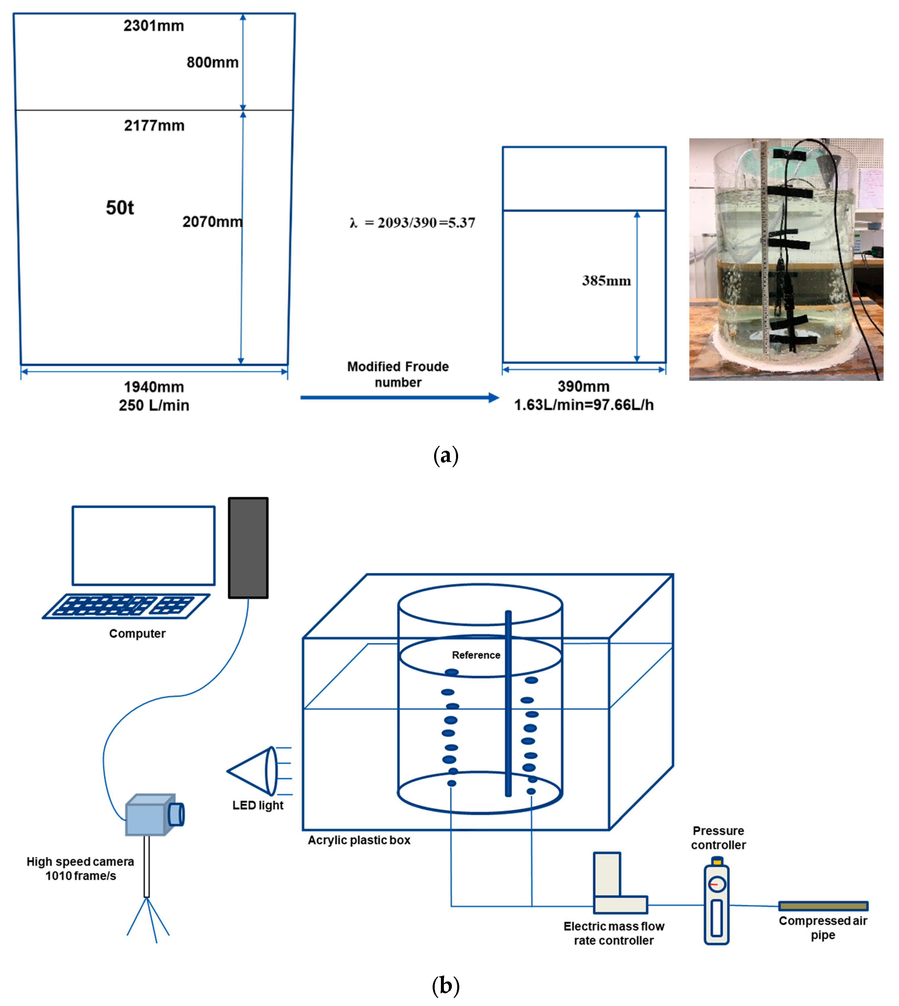
2. Scaling Criterion and Experimental Apparatus

The connection between physical modelling experiments and industrial trials is the scaling criterion. In this study, water and air, at room temperature, were used to represent molten steel and argon, respectively. For the gas injection scaling, the ratio of the inertial and buoyancy forces in the plume was considered to achieve a flow similarity. Using the geometric similarity ( λ = L water   vessel L steel   ladel ) and modified Froude number F r m = ρ gas 2 Q 2 ρ liquid 2 g H d 0 4 [21], the flow rates in the prototype and water experiment can be correlated as follows:
Q air = ( ρ argon ρ water d water 2 ρ air ρ steel d steel 2 H water H steel ) Q argon
where dwater is the plug diameter in the physical modelling, dsteel is the plug diameter in the prototype, ρair and ρwater are the densities of air and water, ρargon and ρsteel are the densities of argon and steel, Hwater is the filled water height, Hsteel is the filled molten steel height, Qair is the air flow rate in the physical modelling (NL·min−1), and Q argon is the effective flow rate in the prototype (L·min−1).
In several works [13,15], the effects of temperatures and pressures on the scaling corrections were also studied. The temperature and pressure are taken into consideration by using the ideal gas law pV = nRT and pin = p0 + ρsteelgHsteel, respectively. Overall, the scaling criterion is derived as follows:
Q air = ( ρ argon ρ water d water 2 ρ air ρ steel d steel 2 H water H steel ) T in T 0 p 0 p in Q argon
where T0 is the normal temperature (273 K), Tin is the molten steel temperature in the prototype (1873 K), p0 is the normal pressure (101,325 Pa), pin is the bottom injection pressure in the prototype (Pa), and Qargon is the flow rate under normal conditions in the prototype (NL·min−1).
All parameters in the physical model were linked to the dimensions of a 50 t steel plant by using a ratio of 5.37. The gas bubbling was given by two porous plugs located at the bottom of the reactor, as shown in Figure 1a. The radial position of the porous plugs, corresponding to that in the industrial ladles, was at a distance of 0.65R, where R is the ladle radius. The radial angles of the dual plugs, α, were chosen as 90°, 135°, and 180°, respectively. Moreover, two probes were positioned at α/2 and 180 + α/2. First, the bubble-size distribution was analyzed using a high-speed camera (Motion Blitz Cube 4), which could take 1010 frames per second. The scaled ladle was placed in an acrylic plastic box, which could decrease the effect of light refractions on the size measurement. Moreover, a pipe with a diameter of 8 mm was fixed in a proper position to be used as a reference. A schematic diagram of the experimental apparatus is shown in Figure 1b. In the mixing-time section, the saturated NaCl solution was used as a tracer to represent the alloy in the ladle process. In each case, a volume of 50 mL of NaCl solution was injected through a funnel. The funnel was located above one of the gas injection plumes close to the water’s surface. In addition, two conductivity probes were located at two feature points to measure the conductivity in the water. Furthermore, a color dye with a density of around 1100 kg/m3 was added through the funnel, at the same position, to show the flow pattern in the ladle. Because it is difficult to determine whether the color dye’s effective diffusion is the same as that of a saturated NaCl solution, the experiments of color dye and saturated NaCl solution were conducted, respectively.

3. Mathematical Modelling and Calculation Methods

In order to predict the flow pattern and mixing condition, a three-dimensional model was established using the commercial software ANSYS FLUENT 19.2 (ANSYS, Canonsburg, PA, USA). The mesh sensitivity was checked by using a method presented in recent publications [22,23]. Meshes with a grid number of approximately 165,000 were used in the simulations. On one side, the Euler–Lagrange model was also used to predict the flow pattern in the same work [22]. On the other side, the mixing condition was calculated by using the species transport model [18,24]. The solution method was also the same as used in previous works [18,22]. The calculations were carried out on a Linux PC, using an Intel E5-2680 CPU with a frequency of 2.50 GHz. The calculations of flow patterns and mixing conditions in each case took approximately two weeks when using a parallel processing mode.

4. Results and Discussion

In the industrial process, the flow rate of the argon injection was in the range of 150~250 NL·min−1. Based on the scaling criterion in Figure 1, the flow rates between the industrial process and water experiments were correlated. In this paper, three conditions of bubbly stirring are linked in Table 2 and later compared to results from physical modelling.

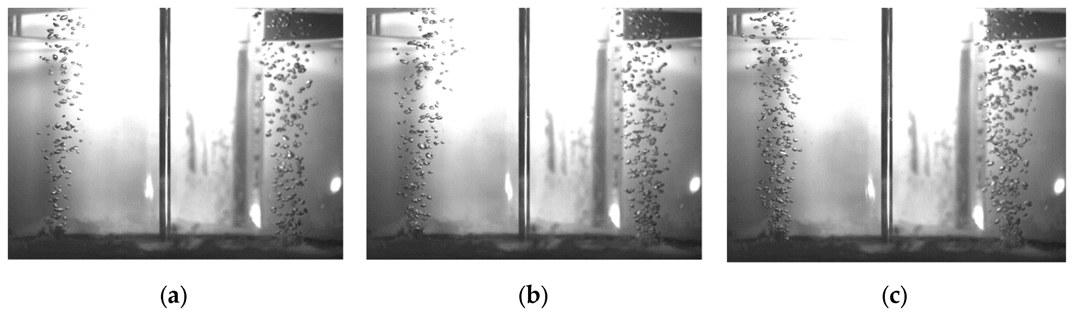
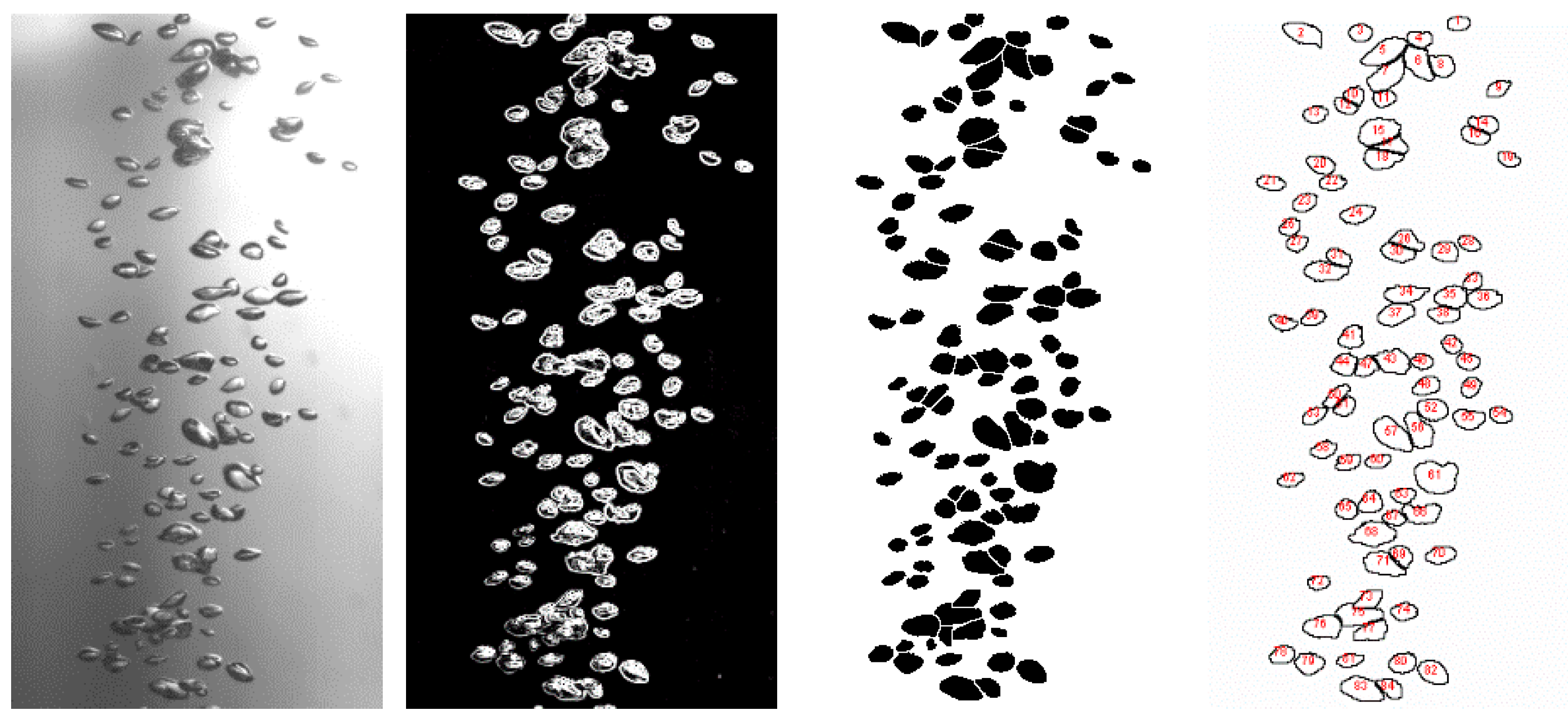
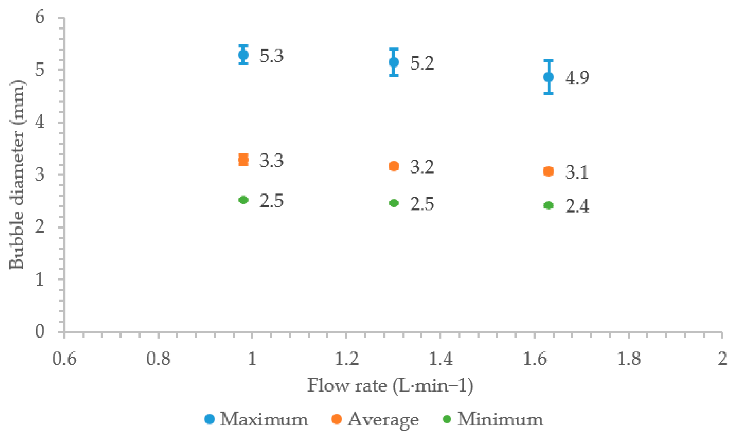
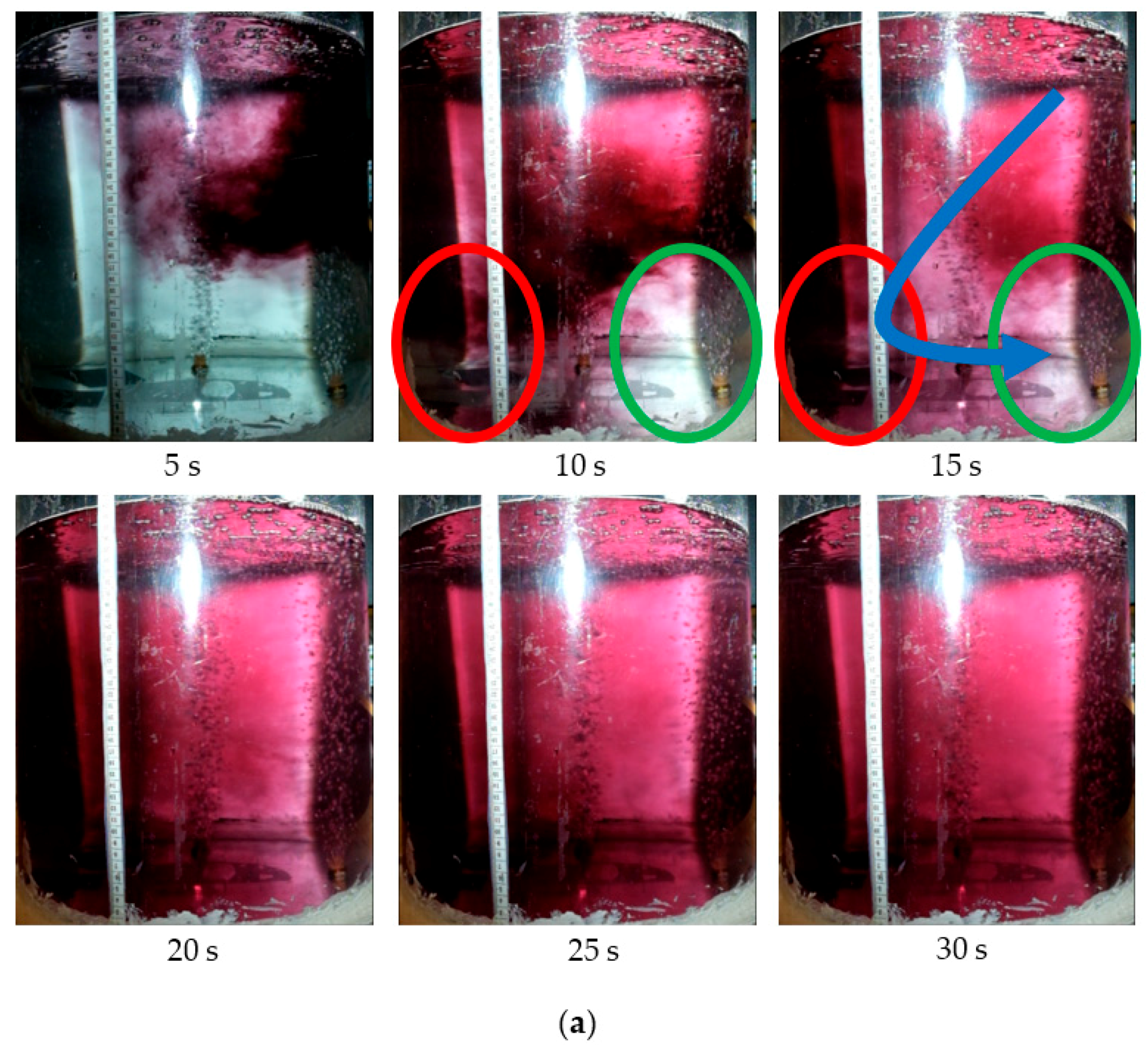
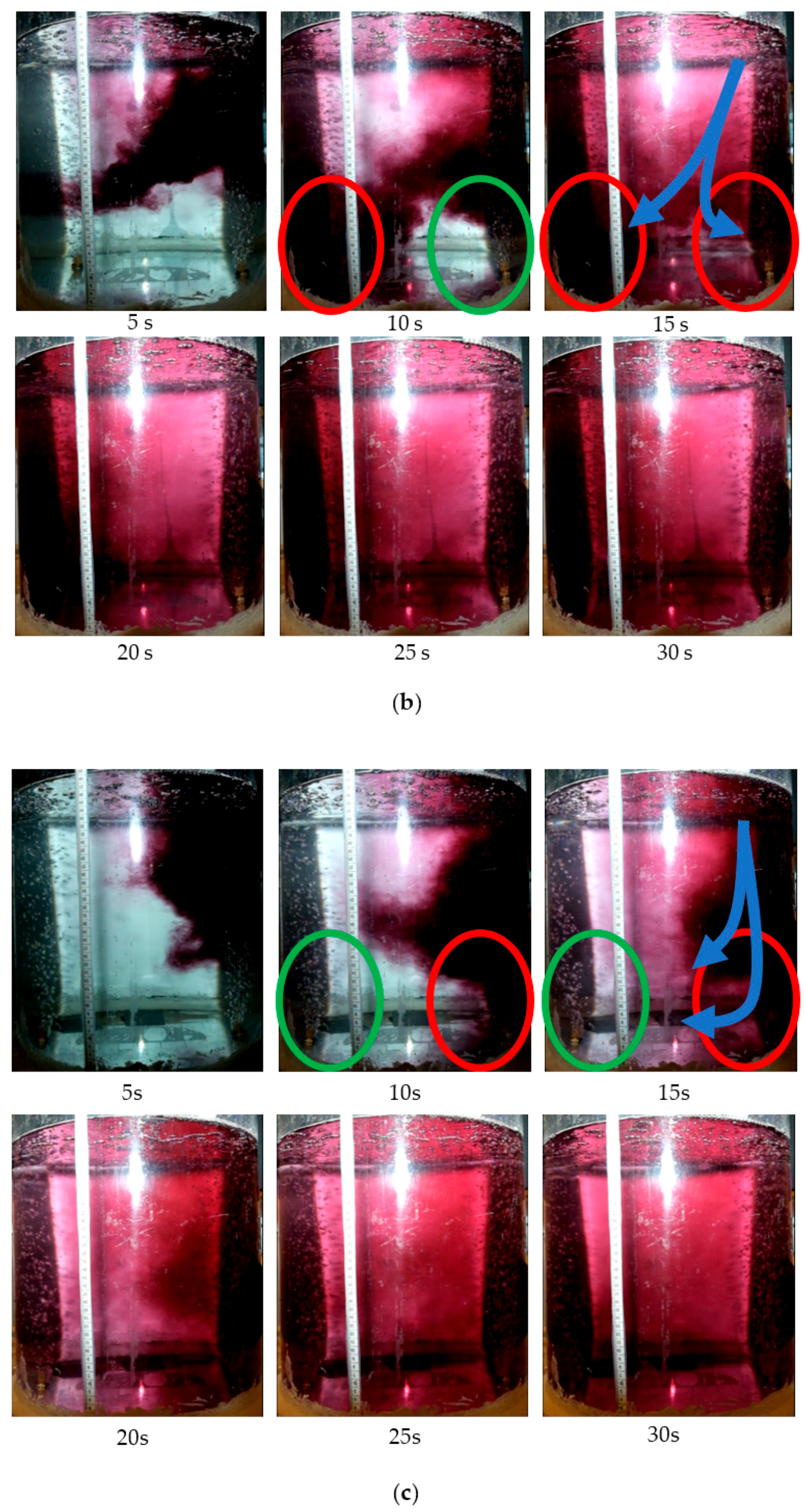
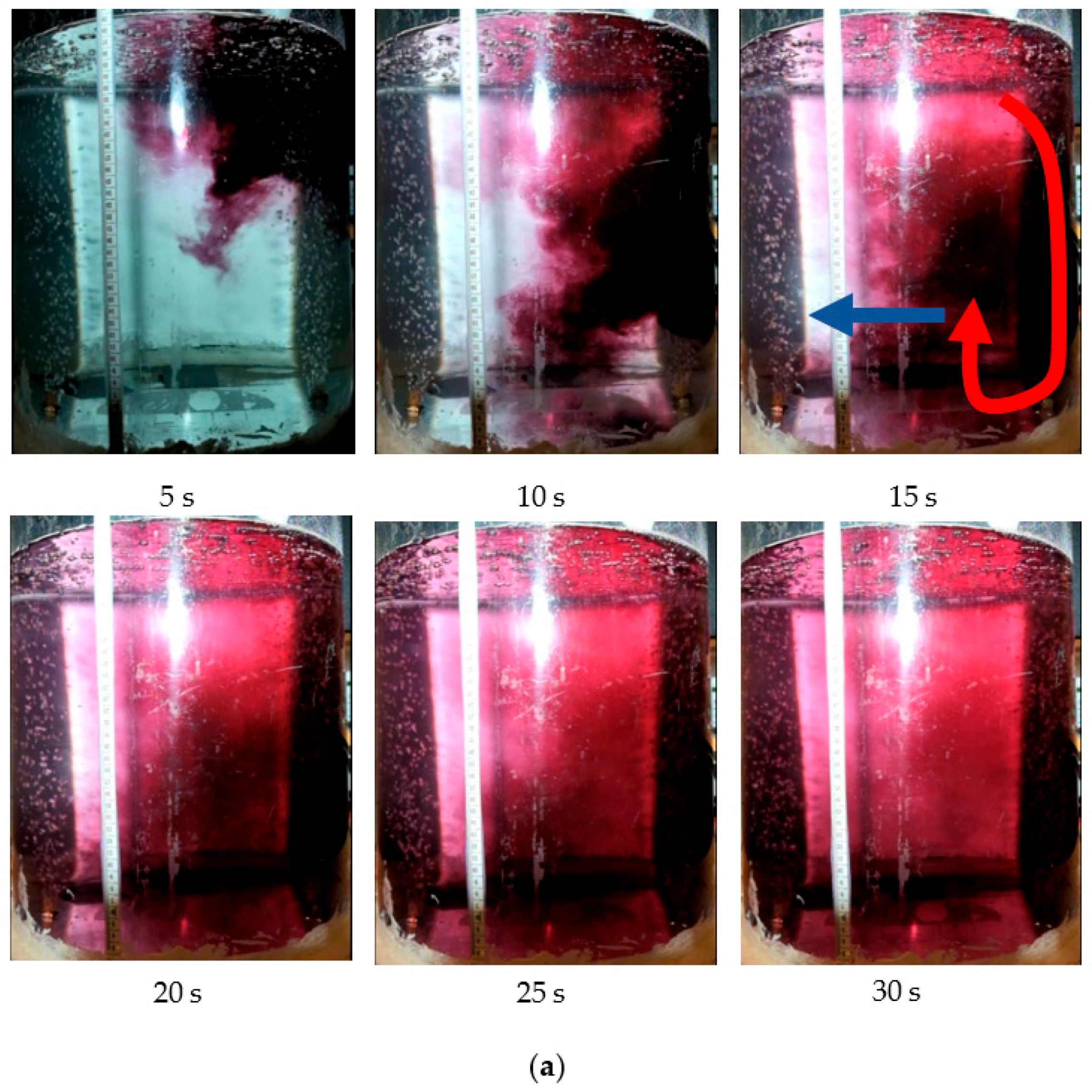
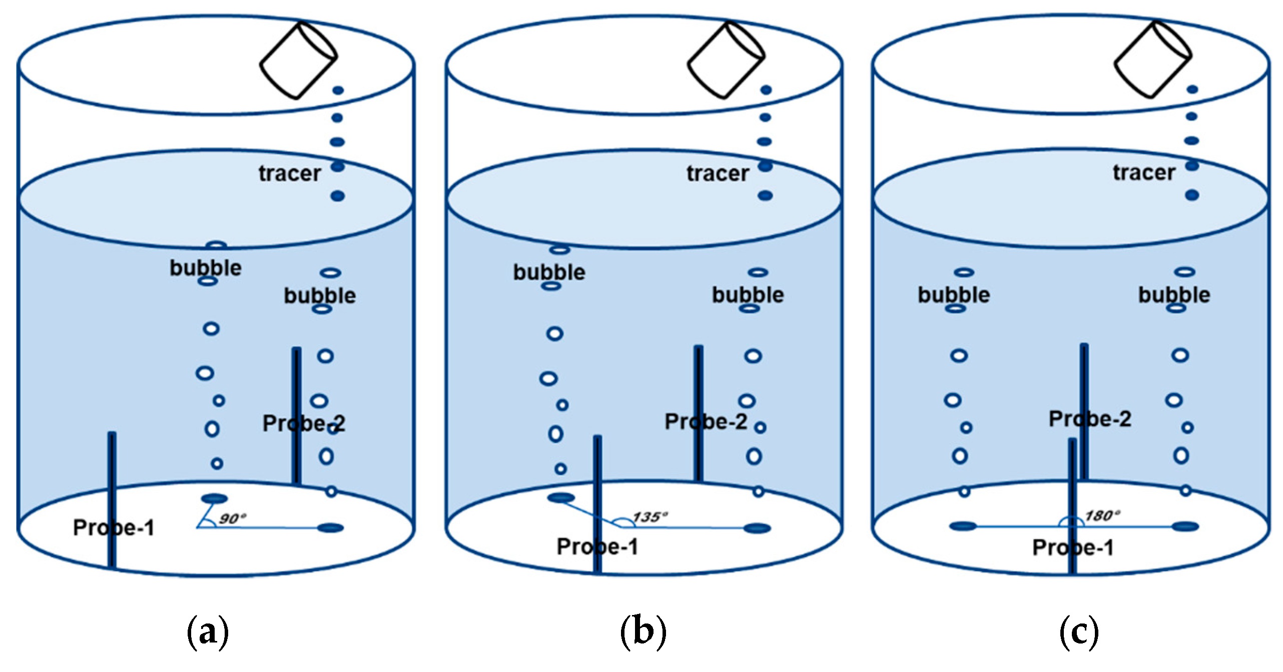
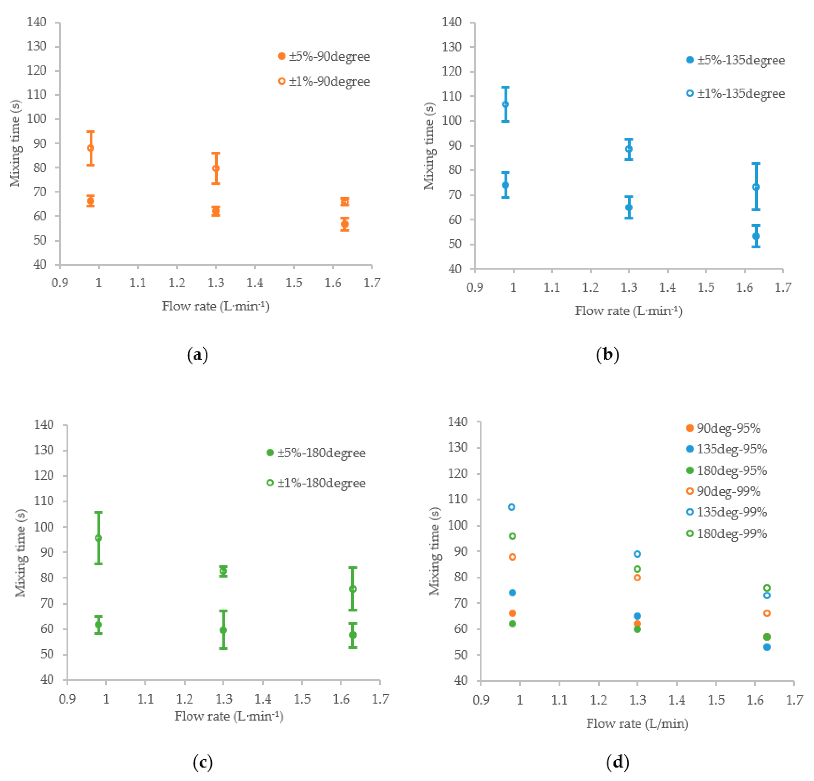
4.1. Gas Bubbling and Mixing Conditions in the Physical Modelling

In the water experiments, the bubbly flow is mainly affected by the bubble’s buoyancy in the fully developed plume zone [25]. The buoyancy, in turn, is closely related to the bubble size, which is not constant in the water experiment; therefore, the bubble-size distribution should be statistically analyzed. The gas injection by porous plugs with various flow rates is shown in Figure 2. According to the size of the reference pipe with a diameter of 8 mm, the gas plume with dispersive bubbles in the middle was chosen, and the bubble size was measured in five figures, under the same flow rate. By using the open-source software ImageJ, the threshold value was adjusted to find the bubble boundaries, and the resulting RGB system figures were converted to binary ones. The post-process of measurement is shown in Figure 3. The maximum, average, and minimum values of bubble sizes are shown in Figure 4. With the flow rate increasing, the minimum bubble size keeps at an around constant value of approximately 2.5 mm, and the maximum and average size only decrease to a small extent. Therefore, the effect of the flow rate on the bubble-size distribution can be neglected in the current cases. Thus, the small effect of the light refraction on the bubble-size measurement was not considered.
The configurations of porous plugs and conductivity probes in the mixing experiment are shown in Figure 5. When the flow pattern reached a quasi-steady state, the NaCl solution was uniformly added to the water. The addition was made at a position corresponding to the position of the open eye, where alloys are added into the molten steel during ladle refining. Because of the bubbles’ random rising, the plume swung periodically. In order to decrease the error of the random gas stirring on the average mixing time, each case was performed three times. After an experiment, the total normalized conductivity curves for two probes were obtained, as shown in Figure 6a. Moreover, the same conductivity curves with a specified range of 0.9~1.1 are shown in Figure 6b. The solid and dashed lines represent the tracer concentration within ±5% and ±1% of the homogenization degrees’ value, respectively. For the ±5% homogenization degree case, the mixing time was determined as the concentration of the tracer, which was continuously within ±5% of a well-mixed bulk value [2]. The procedure was the same for the case of a ±1% homogenization degree case, but the mixing time corresponded to a ±1% well-mixed bulk value.
The mixing times under various flow rates are shown in Figure 7. As the flow rate increases, both the times for ±5% and ±1% homogenization degrees decrease by 7% to 32%. Actually, in terms of the precision of the water experiments, the ±5% homogenization degree was mainly chosen to evaluate the mixing time. For the ±5% homogenization degree, using various configurations in Figure 7d, the averaged mixing time with a radial angle of 180° is always 0% to 7% shorter than that with a radial angle of 90°. Furthermore, the mixing time with a radial angle of 135° decreases the most with an increased flow rate. Nevertheless, under various flow rates, the tendency for the mixing condition for a ±1% homogenization degree is different from that of a ±5% homogenization degree. The reasons for this are discussed in Section 4.3.
For the color-dye experiment, each case was performed once. In the color-dye experiments, the tracer path for a flow rate of 1.63 L·min−1 is shown in Figure 8. In the figures, the color dye’s concentration at the bottom corner is marked distinctly using red and green circles. The red and green circles correspond to the conditions with high and low concentration, respectively. Moreover, the blue vectors show the tracer’s circulation behavior.
It is shown that, for a 90° angle, the tracer goes to the bottom corner opposite to the tracer injection side at 10 s in Figure 8a. This is because of an intense deflected rotation. Therefore, the tracer returns to the injection side along the bottom of the vessel at 15 s. Moreover, for the 135° angle, the off-centered rotation is weaker compared to that for a 90° angle. Some of the tracer is dispersed to the central bottom position at 10 s in Figure 8b, and the remaining tracer is transported to the bottom corner at the injection side at 15 s. However, the condition for a 180° angle is largely different from those of the two other conditions. Because the flow pattern is ideally symmetric when using a 180° angle, the tracer is first mixed at the injection side at 10 and 15 s in Figure 8c. Then, it gradually diffuses and is directed toward the other side of the vessel.

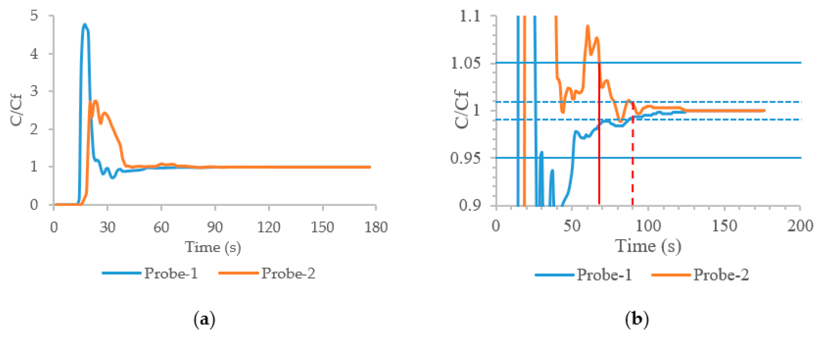
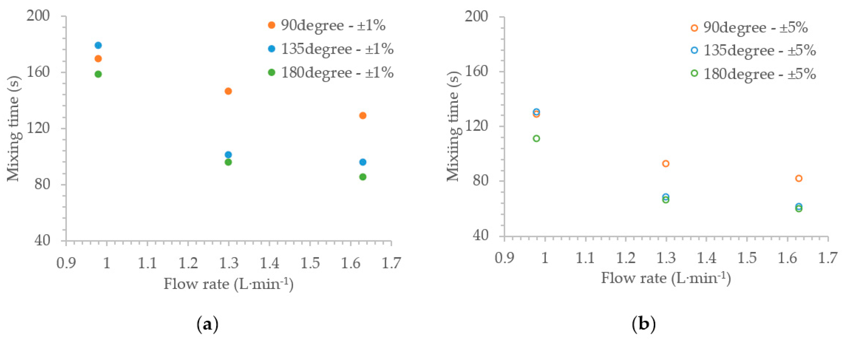
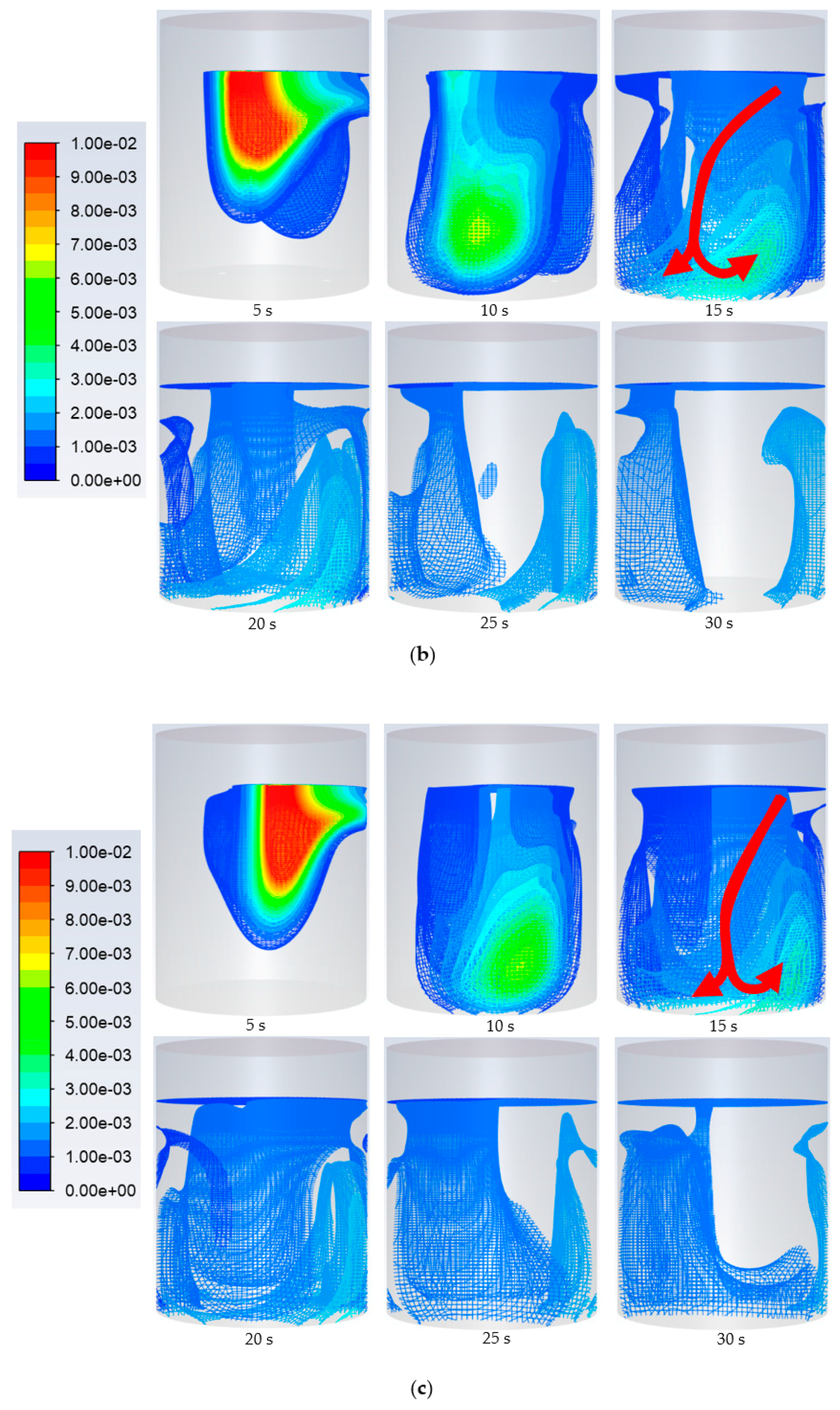
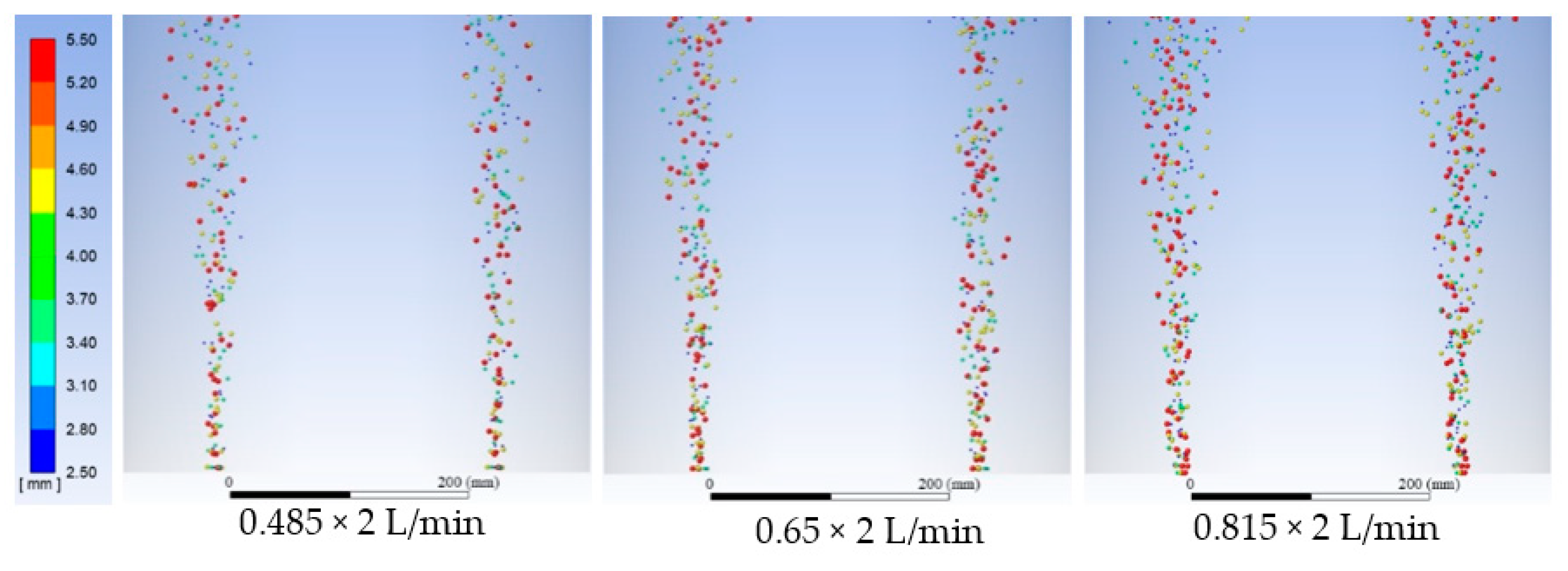
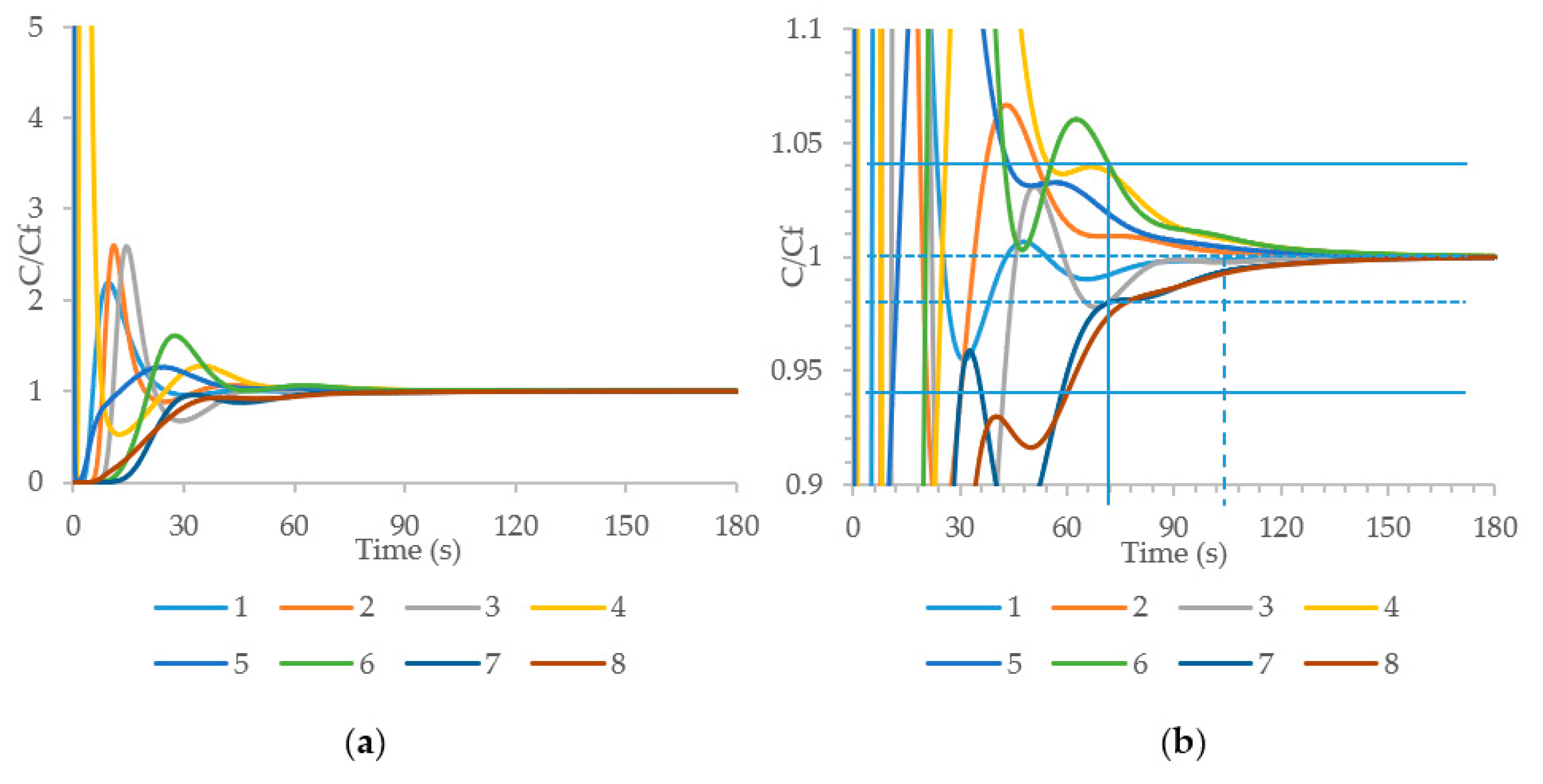
4.2. Calculated Gas Bubbling and Mixing Conditions Using Mathematical Modelling

From previous mathematical modelling, it is clear that the bubble size has some influence on the multiphase interface forces and flow pattern [22]. However, according to the results from the physical modelling, the effect of the flow rate on the size distribution of bubbles injected by the porous plug could be ignored. The bubble-size distribution is within the range of 2.5~5.5 mm, and the average bubble size is 3.5 mm. In the mathematical modelling, the Rosin–Rammler algorithm [24] was used to set up the bubble-size distribution. The bubble injection for various flow rates is shown in Figure 9.
The mixing condition in the ladle is predicted using the species transport model. Several feature points are chosen to monitor the mass fraction of tracers in each zone. For example, the locations of points corresponding to a radial angle of 135° are shown in Figure 10. Also, the normalized curves of the mass fraction at each point are shown in Figure 11. The method to post-process the calculation data was the same as that for the experimental results. The solid and dashed lines correspond to the normalized mass fractions of tracers within the ±5% and ±1% homogenization degrees, respectively.
In the mathematical modelling, the momentum model coupled with the multiphase model is used to calculate the flow pattern. Thereafter, using a fixed flow pattern, the species model is employed to predict the tracer homogenization. Therefore, the flow pattern is the main driver for the tracer diffusion and convection. However, the influence of the tracer’s natural convection, such as the tracer density and temperature, on the mixing condition are not properly considered. The mixing time under various flow rates for ±5% and ±1% homogenization degrees are shown in Figure 12. As can be seen, an increased flow rate results in a large decrease of the mixing time. For the ±5% homogenization degree case and a lower flow rate of 0.98 L·min−1, the mixing time with a radial angle of 180° is approximately 15% shorter compared to a case when using a radial angle of 135°. For a higher flow rate of 1.63 L·min−1, the mixing time for a radial angle of 180° is 27% shorter compared to a case using a radial angle of 90°. Moreover, the reduction of the mixing time is approximately 53% larger for a radial angle of 135°. The results from the mathematical modelling are consistent with those from the physical modelling. When using various radial angles, the variation of mixing times in the ±1% homogenization degree experiments are the same as those in the ±5% homogenization degree experiments. For the ±1% homogenization degree, the smallest and largest variations are approximately 24% and 46% for radial angles of 90° and 135°, respectively.
In addition, the species transport results are also used to show the bubbly flow pattern in Figure 13. The red vectors correspond to the tracer’s mixing patterns. For a radial angle of 90°, the species transport is controlled by a large circulation, as shown in Figure 13a. This is due to the intense deflected flow. The tracer rotates directly to the side away from the injection side, along with the gas–liquid interface, and thereafter recirculates along the wall. Compared to the results for a radial angle of 90°, the flow pattern changes into two rotation flows for a radial angle of 135°, as shown in Figure 13b. Therefore, the tracer is also divided into two parts, and it gradually diffuses at the same time. For a radial angle of 180°, the flow pattern in the ladle is symmetric. Most of the tracer rotates at the injection side and gradually diffuses to the other side, as shown in Figure 13c. Comparing the conditions under various flow rates, the flow pattern predicted by the mathematical modelling agrees well with the results from the physical modelling.
The mixing times in the physical and mathematical modelling are collected in Table 3. Due to the comparison, the mixing time predicted by the mathematical modelling in each condition is always less than that predicted by the physical modelling. Therefore, some parameters in the Euler–Lagrange approach, such as drag coefficient, need to be modified further. Moreover, the main errors between physical modelling results and mathematical modelling results exist under the conditions of the low flow rate and the separation angle of 90 degrees. The discussion of the error is in the next section.

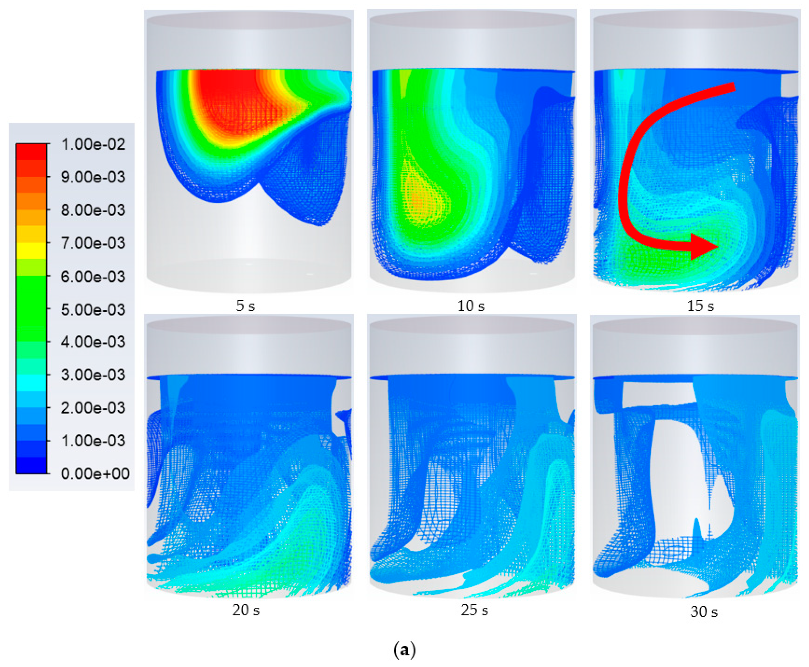
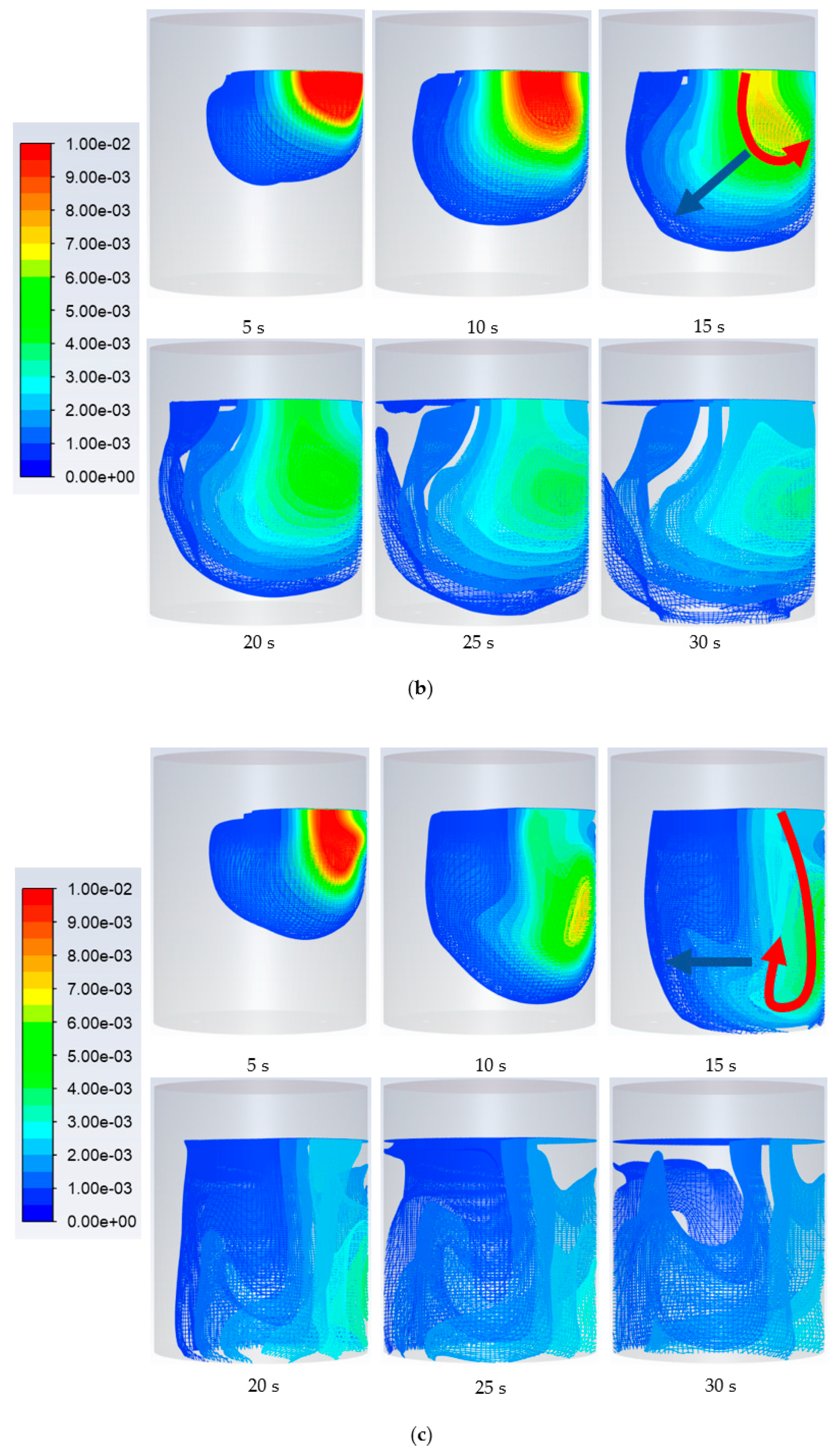
4.3. Convection and Diffusion

For the tracer mixing in the water experiment, the convection and diffusion of tracers took place at the same time. Because the experiment was conducted at room temperature, the effect of temperature on the diffusion rate does not need to be taken into consideration. In the mathematical modelling, the tracer homogenization was controlled by several factors, as shown in Table 4. Compared to the laminar diffusion rate, the turbulent diffusion rate is much higher [26]. Therefore, there are three factors, namely the bubbly flow forced convection, natural convection, and turbulent diffusion, which determine the homogenization degree in the ladle. Under high flow rates, the bubbly flow forced convection is the foremost cause of the tracer’s mixing compared to the contributions from natural convection and turbulent diffusion. However, for low flow rates, the natural convection and turbulent diffusion also influence the homogenization of the tracers. Both for the mathematical modelling and physical modelling results, an increased flow rate resulted in a decreased mixing time for a radial angle of 135°. This is because two stirring rotations can increase the surface of the tracer diffusion. In most of the previous works [5,8,9,12,13,14,16], NaCl or KCl solutions were used as the tracers to determine the mixing time by monitoring the conductivity in the physical modelling trials. Nevertheless, the tracer’s density is larger than that of normal water. Concerning the effect of the tracer’s density on its homogenization pattern, the conditions with and without fixed flow pattern were compared in the mathematical modelling, as shown in Figure 14. The red and blue vectors correspond to the convection pattern and the diffusion pattern, respectively. In comparison to the species transport with and without fixed flow patterns, the latter agrees better with the physical modelling results. Here, the effect of the tracer’s density on its mixing pattern is considered. The result shows that the influence of the alloy’s natural convection on its homogenization pattern cannot be neglected, especially for ‘soft bubbling’ conditions, using low flow rates. In terms of the physical modelling, it is complicated to relate the tracer’s density to the alloy’s density used in the industrial process; therefore, it could be more accurate if the mathematical modelling is validated with data from the physical modelling and thereafter is used to predict the industrial conditions, instead of using physical modelling to predict industrial conditions. Furthermore, in the ladles with different volumes, the contributions of convection and turbulent diffusion on the mixing pattern should be analyzed in more detail in the future.
Bold terms are the controlling parameters of each term in mathematical modelling.
Moreover, for the ladles with various weights, the optimal radial positions and separation angles of the plugs were collected in previous works [5,7,8,9,11,12,13,14,16,19,20], as shown in Figure 15. In terms of the mixing condition, an optimal range of plug’s radial location is mainly off-centered for a single plug injection at values ranging from 0.72R to 0.75R. For dual-plug injections, a separation angle between the plugs of approximately 160° is mostly recommended, and the optimal dual-plug radial position is around 0.65R. Overall, larger radial angles in the range of 135~180° are recommended to reach a bubbly stirring condition when using dual porous plugs.

5. Conclusions

The bubbly flow and tracer mixing in a 50t ladle were studied based on physical and mathematical modelling. The effects of tracer convention and diffusion on the mixing pattern were discussed. For a ±5% homogenization degree, the effect of convection on the mixing pattern is most important. Also, the mixing time using dual plugs positioned at a radial angle of 180° is shortest. In addition, the mixing time when using dual plugs positioned with a radial angle of 135° decreased most with an increasing flow rate, among the various conditions. In addition, a comparison of the conditions for various flow rates shows that the flow pattern predicted by the mathematical modelling agrees well with the physical modelling results. For a ±1% homogenization degree, the influence of the alloy’s natural convection on its homogenization pattern cannot be neglected, especially for a ‘soft bubbling’ condition using a low flow rate. Furthermore, in the ladles with different weights, the effect of convection and diffusion on the mixing should be studied in more detail. In comparison to the previous works, it is recommended that a larger radial angle in the range of 135°~180° is chosen to obtain bubbly stirring conditions when using dual porous plugs.

Author Contributions

Conceptualization, H.L., M.E., and P.G.J.; investigation, Y.L. and H.B.; project administration, H.L. and Y.G.; software, Y.L. and H.B.; supervision, H.L., M.E., and P.G.J.; writing—original draft preparation, Y.L.; writing—review and editing, M.E. and P.G.J.

Funding

This research received no external funding.

Acknowledgments

Yu Liu extends his sincere appreciation to the China Scholarship Council for financial support of his study at the KTH-Royal Institute of Technology (Stockholm).

Conflicts of Interest

The authors declare no conflict of interest.

References

  1. Sichen, D. Modelling related to secondary steel making. Steel Res. Int. 2012, 83, 825–841. [Google Scholar] [CrossRef]
  2. Liu, Y.; Ersson, M.; Liu, H.P.; Jönsson, P.G.; Gan, Y. A review of physical and numerical approaches for the study of gas stirring in ladle metallurgy. Metall. Mater. Trans. B 2019, 50, 555–577. [Google Scholar] [CrossRef]
  3. Mazumdar, D.; Guthrie, R.I.L. Mixing models for gas stirred metallurgical reactors. Metall. Trans. B 1986, 17, 725–733. [Google Scholar] [CrossRef]
  4. Mazumdar, D.; Kim, H.B.; Guthrie, R.I.L. Modelling criteria for flow simulation in gas stirred ladles: Experimental study. Ironmak. Steelmak. 2000, 27, 302–309. [Google Scholar] [CrossRef]
  5. Joo, S.; Guthrie, R.I.L. Modelling flows and mixing in steelmaking ladles designed for single-plug and dual-plug bubbling operations. Metall. Trans. B 1992, 23, 765–778. [Google Scholar] [CrossRef]
  6. Krishnakumar, K.; Ballal, N.B.; Sinha, P.K.; Sardar, M.K.; Jha, K.N. Water model experiments on mixing phenomena in a VOD ladle. ISIJ Int. 1999, 39, 419–425. [Google Scholar] [CrossRef]
  7. González-Bernal, R.; Solorio-Diaz, G.; Ramos-Banderas, A.; Torres-Alonso, E.; Hernández-Bocanegra, C.A.; Zenit, R. Effect of the fluid-dynamic structure on the mixing time of a ladle furnace. Steel Res. Int. 2017, 89, 1700281. [Google Scholar] [CrossRef]
  8. Mandal, J.; Patil, S.; Madan, M.; Mazumdar, D. Mixing time and correlation for ladles stirred with dual porous plugs. Metall. Mater. Trans. B 2005, 36, 479–487. [Google Scholar] [CrossRef]
  9. Mazumdar, N.; Mahadevan, A.; Madan, M.; Mazumdar, D. Impact of ladle design on bath mixing. ISIJ Int. 2005, 45, 1940–1942. [Google Scholar] [CrossRef]
  10. Patil, S.P.; Satish, D.; Peranandhanathan, M.; Mazumdar, D. Mixing models for slag covered, argon stirred ladles. ISIJ Int. 2010, 50, 1117–1124. [Google Scholar] [CrossRef]
  11. Amaro-Villeda, A.M.; Ramirez-Argaez, M.A.; Conejo, A.N. Effect of slag properties on mixing phenomena in gas-stirred ladles by physical modelling. ISIJ Int. 2014, 54, 1–8. [Google Scholar] [CrossRef]
  12. Tang, H.Y.; Guo, X.C.; Wu, G.H.; Wang, Y. Effect of gas blown modes on mixing phenomena in a bottom stirring ladle with dual plugs. ISIJ Int. 2016, 56, 2161–2170. [Google Scholar]
  13. Liu, Z.Q.; Li, L.M.; Li, B.K. Modelling of gas-steel-slag three-phase flow in ladle metallurgy: Part I. physical modelling. ISIJ Int. 2017, 57, 1971–1979. [Google Scholar] [CrossRef]
  14. Gómez, A.S.; Conejo, A.N.; Zenit, R. Effect of separation angle and nozzle radial position on mixing time in ladles with two nozzles. J. Appl. Fluid Mech. 2018, 11, 11–20. [Google Scholar] [CrossRef]
  15. Fan, C.M.; Hwang, W.S. Study of optimal Ca-Si injection position in gas stirred ladle based on water model experiment and flow simulation. Ironmak. Steelmak. 2002, 29, 415–426. [Google Scholar] [CrossRef]
  16. Ek, M.; Wu, L.; Valentin, P.; Sichen, D. Effect of inert gas flow rate on homogenization and inclusion removal in a gas stirred ladle. Steel Res. Int. 2010, 81, 1056–1063. [Google Scholar] [CrossRef]
  17. Geng, D.Q.; Lei, H.; He, J.C. Optimization of mixing time in a ladle with dual plugs. Int. J. Miner. Metall. Mater. 2010, 17, 709–714. [Google Scholar] [CrossRef]
  18. Liu, H.P.; Qi, Z.Y.; Xu, M.G. Numerical simulation of fluid flow and interfacial behavior in three-phase argon-stirred ladles with one plug and dual plugs. Steel Res. Int. 2011, 82, 440–458. [Google Scholar] [CrossRef]
  19. Lou, W.T.; Zhu, M.Y. Numerical simulations of inclusion behavior and mixing phenomena in gas-stirred ladles with different arrangement of tuyeres. ISIJ Int. 2014, 54, 9–18. [Google Scholar] [CrossRef]
  20. Duan, H.J.; Zhang, L.F.; Thomas, B.G.; Conejo, A.N. Fluid flow, dissolution, and mixing phenomena in argon-stirred steel ladles. Metall. Mater. Trans. B 2018, 49, 2722–2743. [Google Scholar] [CrossRef]
  21. Krishnapisharody, K.; Irons, G.A. A critical review of the modified froude number in ladle metallurgy. Metall. Mater. Trans. B 2013, 44, 1486–1498. [Google Scholar] [CrossRef]
  22. Liu, Y.; Ersson, M.; Liu, H.P.; Jönsson, P.; Gan, Y. Comparison of Euler-Euler approach and Euler–Lagrange approach to model gas injection in a ladle. Steel Res. Int. 2019, 90, 1–13. [Google Scholar] [CrossRef]
  23. Liu, Z.Q.; Li, B.K. Scale-adaptive analysis of Euler-Euler large eddy simulation for laboratory scale dispersed bubbly flows. Chem. Eng. J. 2018, 338, 465–477. [Google Scholar] [CrossRef]
  24. ANSYS FLUENT Theory Guide Version 19.2; ANSYS Inc.: Canonsburg, PA, USA, 2017.
  25. Castillejos, A.H.; Brimacombe, J.K. Measurement of physical characteristics of bubbles in gas-liquid plumes. 2. local properties of turbulent air-water plumes in vertically injected jets. Metall. Trans. B 1987, 18, 659–671. [Google Scholar] [CrossRef]
  26. Leonard, A. Overview of Turbulent and Laminar Diffusion and Mixing; Springer Vienna: Udine, Italy, 2009; pp. 2–17. [Google Scholar]
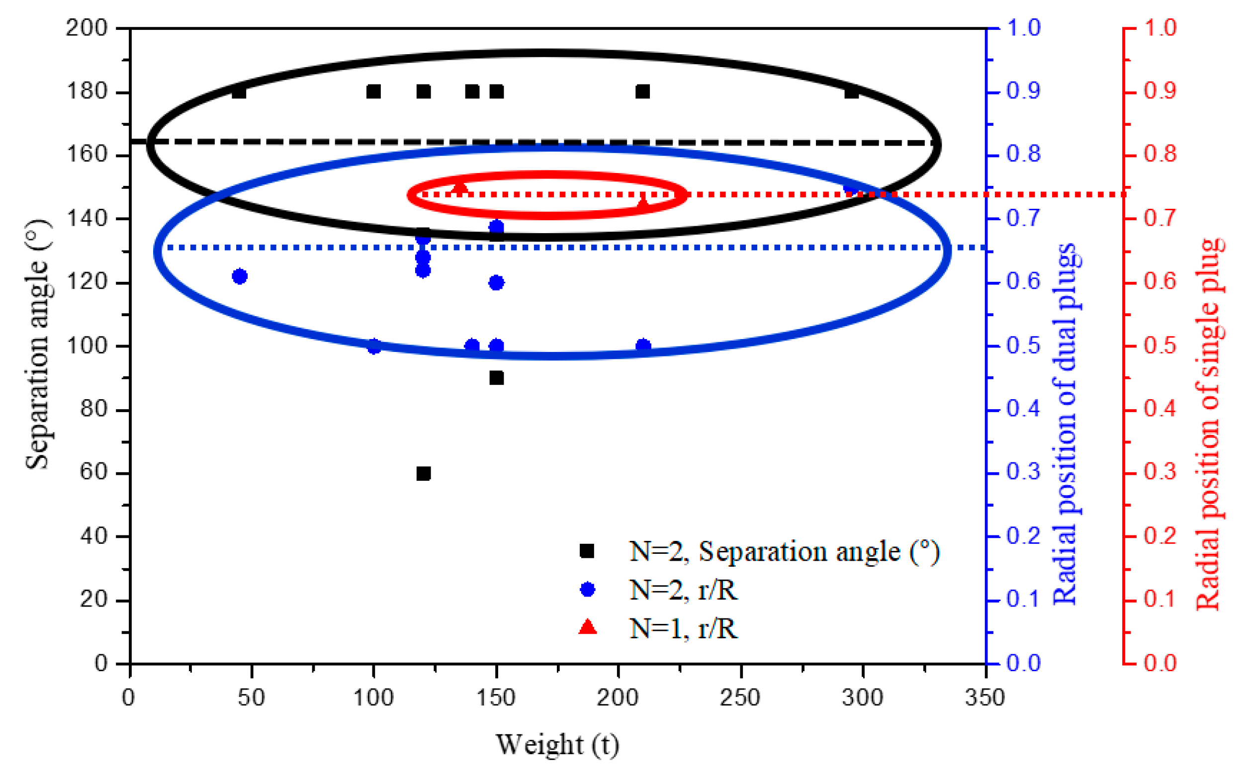
Figure 1. Scaling criterion (a) and experimental apparatus (b).
Metals 09 01136 g001
Figure 2. Gas injection using two porous plugs in the physical modelling: (a) 0.98 L·min−1; (b) 1.30 L·min−1; and (c) 1.63 L·min−1.
Metals 09 01136 g002
Figure 3. Process of bubble-size statistics in ImageJ, under the condition of 1.30 L·min−1.
Metals 09 01136 g003
Figure 4. The maximum, average, and minimum values of bubble size in the water experiment.
Metals 09 01136 g004
Figure 5. Schematic diagram of the porous plugs and conductivity probes’ configurations at radial angles of (a) 90°; (b) 135°; and (c) 180°.
Metals 09 01136 g005
Figure 6. Normalized conductivity curves for two probes for a flow rate of 1.30 L·min−1, using a 135° plug angle. (a) Normalized value with whole range. (b) Normalized value between 0.9 and 1.1.
Metals 09 01136 g006
Figure 7. Measured mixing times at different flow rates with various radial-plug angles: (a) 90°; (b) 135°; (c) 180°; and (d) total.
Metals 09 01136 g007
Figure 8. Color dye path for a 1.63 L·min−1 flow rate when using various radial-plug angles: (a) 90°; (b) 135°; and (c) 180°.
Metals 09 01136 g008aMetals 09 01136 g008b
Figure 9. Color-dye path for a 1.63 L·min−1 flow rate when using various radial-plug angles.
Metals 09 01136 g009
Figure 10. Monitoring point in the mathematical modelling. Ponit1 (0, 0, and 200 mm), Ponit2 (70.8, 170.9, and 20 mm), Ponit3 (−70.8, −170.9, and 20 mm), Ponit4 (170.9, −70.8, and 200 mm), Ponit5 (−170.9, 70.8, and 200 mm), Ponit6 (−117, 0, and 350 mm), Ponit7 (170.9, 70.8, and 350 mm), Ponit8 (−70.8, 170.9, and 350 mm).
Metals 09 01136 g010
Figure 11. Normalized mass fraction curves when using a flow rate of 1.30 L·min−1 and a 135° plug angle. (a) Normalized value in whole range. (b) Normalized value between 0.9 and 1.1.
Metals 09 01136 g011
Figure 12. Measured mixing time with various radial-plug angles in the experiment: (a) ±5% homogenization and (b) ±1% homogenization.
Metals 09 01136 g012
Figure 13. Tracer homogenization for a flow rate of 1.63 L·min−1: (a) 90°; (b) 135°; and (c) 180°.
Metals 09 01136 g013aMetals 09 01136 g013b
Figure 14. Effect of tracer’s natural convection on the mixing pattern for a low flow rate of 0.98 L·min−1: (a) color dye experiment; (b) modelling with a fixed flow pattern; and (c) modelling without a fixed flow pattern.
Metals 09 01136 g014aMetals 09 01136 g014b
Figure 15. Collection of optimal radial position and separation angle of plugs in ladles with various weights. (Points with black color, blue color, and red color represent the data of dual plugs’ separation angles, radial positions of dual plugs, and radial positions of single plug, respectively. The color of point is same as that of the axis.)
Metals 09 01136 g015
Table 1. Physical and mathematical modelling of gas-stirred ladles of different weights.
AuthorWeightScaleGas Injection PatternPlug PositionPlug Radial AngleLiquid MetalGasPhysical ModellingMathematical ModellingOptimal Plug Number and Position
Water-based solutions
Liu et al. [13]45 t1/3porous plug0R, 0.5R, 0.56R, 0.62R, 0.67R, 0.73R60°, 90°, 120°, 150°, and 180°waterN2NaCl above the exposed eye-N = 2, 0.5R~0.73R-180°
Joo and Guthrie [5]100 t1/3porous plug0R, 0.33R, 0.5R, 0.67R45°, 90°, 135°, and 180°waterairKCl above the plumeEuler–Euler + species (own code)N = 2, 0.5R-180°
Tang et al. [12]120 t1/3porous plug0.55R, 0.64R, 0.70R45°, 90°, 135°, and 180°waterN2KCl above the exposed eyeVOF + species (Fluent)N = 2, 0.7R-180°, 0.64R-135°, and 0.55R-180°
Gómez et al. [14]120 t1/8nozzle1/3R, 1/2R, and 2/3R60°, 120°, and 180°waterairKCl above the exposed eye-N = 2, 0.67R-60°
González-Bernal et al. [7]135 t1/7Tuyere1/3R, 2/3R, and 3/4R60°waterairvegetal red colorant at the central bottom-N = 1, 3/4R
Mandal et al. [8]140 t1/5tuyere/nozzle0R, 0.5R-waterair/N2NaCl or H2SO4 axis of symmetry-N = 2, 0.5R-180°
Amaro-Villeda et al. [11]140 t1/6Nozzle0R, 0.33R, 0.5R, 0.67R, 0.8R120°, 180°waterairNaOH or HCl-N = 2, 0.5R-180°
Mazumdar et al. [9]210 t0.17Nozzle0R, 0.5R, and 0.64R90°, 180°waterair/N2NaCl or H2SO4 axis of symmetry-N = 2, 0.5R-180°
Ek. et al. [16]200 t1/5porous plug0.72R-waterairNaCl above the plumeEuler–Euler + species (Comsol)N = 1, 0.72R
This work50 t1/5.37porous plug0.65R90°, 135°, and 180°waterairNaCl and red dye above the open eyeEuler–Lagrange + species (Fluent)-
Steel-based solutions
Liu et al. [18]150 t-porous plug0.687R90°, 135°, 180°steelargon-Euler–Lagrange + species (Fluent)N = 2, 0.687R-180°
Luo et al. [19]150 t-Nozzle0.3R, 0.4R, 0.5R, 0.6R, 0.7R, 0.8R45°, 90°, 135°, and 180°steelargon-Euler–Euler + species (Fluent)N= 2, 0.6R-135°
Duan et al. [20]150 t-porous plug0.34R, 0.5R, 0.68R, 0.75R45°, 90°, 135°, and 180°steelargon-Euler–Lagrange + species (Fluent)N = 2, 0.5R-90°
Geng et al. [17]295 t-Nozzle0.25R, 0.33R, 0.5R, 0.75R, and 0.8R90°, 120°, 150°, and 180°steelargon-Euler–Euler +species (CFX)N = 2, 0.75R-180°
Table 2. Various flow rates in the industrial process and scaled values in the water experiment.
CasesFlow Rate (L·min−1)
Industrial Process150200250
Water experiment0.981.301.63
Table 3. Comparison of the tracer homogenization in the physical and mathematical modelling.
-Flow Rate (L·min−1)Mixing Time (s)
90 degree135 degree180 degree
PhysicalNumericalErrorPhysicalNumericalErrorPhysicalNumericalError
±5%0.9866129.396%74130.576%6211179%
1.36292.349%6568.76%6066.210%
1.63578244%536115%57605%
±1%0.988816992%10717967%9615864%
1.38014683%8910113%839616%
1.636612995%738516%768512%
Bold terms are in the large error ratio between the physical modelling and mathematical modelling.
Table 4. Factors that affect the tracer homogenization in the mathematical modelling.
Species TransportFactorExpression
Mass diffusionLaminar diffusion ρ × D lam × S i
Turbulent diffusion μ t S c t × S i
ConvectionBubbly flow forced convection ( ρ × v × S i )
Natural convection t ( ρ × S i ) + ( ρ × v × S i )
Bold terms are the controlling parameters of each term in mathematical modelling.

