Experimental Determinations of Mixing Times in the IronArc Pilot Plant Process

Abstract

IronArc is a newly developed technology and an emerging future process for pig iron production. The long-term goal with this technology is to reduce the CO₂ emissions and energy consumption compared to existing technologies. The production rate of this process is dependent on the stirring, which was investigated in the pilot plant process by measuring the mixing time in the slag bath. Moreover, slag investigations were done both based on light optical microscope studies as well as by Thermo-Calc calculations in order to determine the phases of the slag during operation. This was done because the viscosity (which is another important parameter) is dependent on the liquid and solid fractions of the slag. The overall results show that it was possible to determine the mixing time by means of the addition of a tracer (MnO₂ powder) to the slag. The mixing time for the trials showed that the slag was homogenized after seconds. For two of the trials, homogenization had already been reached in the second sample after tracer addition, which means ≤8 s. The phase analysis from the slag indicated that the slag is in a liquid state during the operation of the process.

1. Introduction

Submerged gas injection is used in many pyrometallurgical processes and serves several purposes. The gas creates stirring and mixing in the bath, which increases the kinetics, the distribution of the reduction agents, the refinement of the bath, as well as inclusion removal. The mixing time is often used as a measurement of how well the liquid bath is stirred, which has been investigated extensively for different production processes within the steel industry.

IronArc is an emerging future technology developed by ScanArc in Sweden to produce pig iron [1]. In the current pilot scale process, submerged gas injection is used through a plasma generator into a liquid slag bath consisting of magnetite and hematite. The hematite and magnetite are firstly transferred into the cylindrical reactor and melted using hot gas consisting of liquefied petroleum gas (LPG) and air that are injected into the reactor. The injected gas has an approximate temperature of 3500–4000 °C when leaving the plasma generator. CO gas and H₂ gas are created when the LPG is heated together with air and is used as a reductant in the reduction step where hematite and magnetite is reduced to wüstite. Then, carbon is used as reductant for the final reduction step where wüstite is reduced to pig iron. The reaction steps for this process can be seen in Equations (1)–(5).

$${\mathrm{Fe}}_3{\mathrm{O}}_4\left(\mathrm{s}\right)+\mathrm{CO}\left(\mathrm{g}\right)=3\mathrm{FeO}\left(\mathrm{l}\right)+2{\mathrm{CO}}_2\left(\mathrm{g}\right)$$

(1)

$${\mathrm{Fe}}_3{\mathrm{O}}_4\left(\mathrm{s}\right)+{\mathrm{H}}_2\left(\mathrm{g}\right)=3\mathrm{FeO}\left(\mathrm{l}\right)+{\mathrm{H}}_2\mathrm{O}\left(\mathrm{g}\right)$$

(2)

$${\mathrm{Fe}}_2{\mathrm{O}}_3\left(\mathrm{s}\right)+\mathrm{CO}\left(\mathrm{g}\right)=2\mathrm{FeO}\left(\mathrm{l}\right)+{\mathrm{CO}}_2\left(\mathrm{g}\right)$$

(3)

$${\mathrm{Fe}}_2{\mathrm{O}}_3\left(\mathrm{s}\right)+{\mathrm{H}}_2\left(\mathrm{g}\right)=2\mathrm{FeO}\left(\mathrm{l}\right)+{\mathrm{H}}_2\mathrm{O}\left(\mathrm{g}\right)$$

(4)

$$\mathrm{FeO}\left(\mathrm{s}\right)+\mathrm{C}\left(\mathrm{s}\right)=\mathrm{Fe}\left(\mathrm{l}\right)+\mathrm{CO}\left(\mathrm{g}\right)$$

(5)

This new technology uses plasma generators that are powered by electric energy, which opens the possibility of using renewable resources. Since the input material is melted at high temperatures, a wide range of shapes of the input material can be used, from very fine particles to larger material pieces. Thereby, the physical properties of the input material are not a concern for the feeding and melting of the added materials. Furthermore, preliminary calculations have shown that this new technology has the possibility to reduce the energy consumption compared to existing technologies used for pig iron production [1].

As a result of the importance of the mixing in this new process, detailed information about the stirring and fluid flow is of great interest for the process development. In addition, the mixing in the process is important for future upscaling of the process to an industrial level. This process has been investigated in two earlier studies [2,3]. In one of the studies [2], a 1/3 scale water model was used to investigate both the penetration depth of the injected gas and also the mixing time. In the second investigation [3], the penetration depth of the injected gas was investigated. Furthermore, the mixing time has been previously investigated for several metallurgical processes and it provides important knowledge with respect to the homogenization of liquid baths [4,5,6,7,8,9,10,11,12,13,14,15]. Small scale water modelling has almost exclusively been used for the determination of the mixing time and most models have been scaled from 1:3 to 1:10 of that of the actual reactors. However, the mixing time has not been investigated to a large extent in actual full-scale processes within the steel industry, especially when measuring the tracer content as a function of time. Furthermore, it was not possible to find investigations in the open literature where experiments were performed in a slag bath of an industrial process where a tracer was used to determine the mixing time. In some investigations, radiotracers have been used to measure the efficiency of mixing in various industries, such as petrochemicals, oil and gas, and wastewater plants. In these cases, the radiotracer is injected at the inlet and thereafter monitored at the outlet, which enables a determination of the mixing efficiency [16,17].

This new technology demands sufficiently powerful and fast mixing and in turn a short mixing time in order to have a competitive production rate. Therefore, the mixing time was determined in the IronArc pilot plant based on industrial trials in the pilot plant process using a non-radiative tracer. Furthermore, the importance of these investigations, with mixing time experiments in a high-temperature environment and pilot plant experiments, goes beyond this particular process. As a result of the infrequent number of investigations of mixing time determinations by tracer addition in industrial processes, at least in the open literature, these experiments are therefore of interest for other gas stirred processes as well. In addition, these results play an important role in upscaling, since they can be used as validation for numerical models that predict the mixing time for a gas–slag system.

2. Materials and Methods

2.1. Overall Description of Experimental Procedure

The mixing time in the IronArc pilot plant process was investigated in plant trials by adding a tracer to a liquid slag and by measuring the tracer concentration over time, as it became homogenized in the slag due to the stirring and mixing created by the injected gas through a submerged nozzle placed horizontally on the reactor wall. This was done by taking continuous slag samples after the addition of the tracer and noting the time for each sample. When the tracer concentration in the slag had reached its final value, the homogenization time, i.e., the mixing time, could be determined.

First, a small amount of the input material was transferred into the reactor and was then melted to a slag. Thereafter, a continuous feeding of the remaining material proceeded. To determine the mixing time of the process at this stage, a tracer was added to the molten slag when the flow in the slag was fully developed and all the material had been fed in and melted into a slag. The tracer was added from a hole in the roof in all of the trials. Moreover, it needed to be added in three different plastic containers since it was not possible to add a sufficient amount of tracer using only one container. As soon as the tracers were added, the time was noted. Then, samples of the slag were taken with a sampling rod and the time for each slag sample was logged. When all the samples were taken, the tracer content in the samples were measured by XRF-analysis. This was done with a fully integrated energy dispersive XRF analyzer, Epsilon 1 Mining from PANalytical (PANalytical, Almelo, The Netherlands). Moreover, the time when the samples had reached the final tracer content in the bath was defined as the mixing time. All sampling rods consisted of approximately 0.5 cm diameter rebars and they were each marked so that all samples were taken at the same bath depth. They were also numbered to keep track of all the samples. During solidification, the samples were placed with a safe distance between each on the brick floor, in order to prevent contamination. The experiment was performed under oxidizing conditions, since only the mixing time was of interest and not the yield of different elements in the process. A schematic figure of the sampling procedure can be seen in Figure 1. It shows how the tracer spreads in the slag over time as well as how continuous sampling was done throughout the experiment.

The chosen tracer was a MnO₂ powder with a diameter in the order of micrometers. It was chosen because of the low amount of MnO in the initial slag and its low melting temperature. The low initial amount of MnO in the slag assured that the addition of MnO₂ powder would appear in the examination of the samples, after the tracer had been added to the bath. MnO₂ has a melting temperature around 535 °C [18] and it decomposes to other MnO-compounds at higher temperatures. This means that it melts quickly and forms Mn₃O₄ or MnO depending on the available oxygen at the operating temperature, which is a result of the high temperatures and small powder diameters [18,19]. It was important to use a tracer with low melting point, since too high a melting point would result in overly long dissolution times of the tracer in the slag bath. This, in turn, would make it difficult to determine the mixing time. Specifically, since the time for mixing of the bath was of interest and not the dissolving time of the added powder.

A total of five different trials were performed, as summarized in

Table 1. Overall sampling procedure for the five mixing-time trials.

Trial	1	2	3	4	5
Number of samples after tracer	13	13	5	5	10
Time between samples	1 min	1 min	Sampling as fast as possible

. The table also shows an overview of the different sampling procedures for all trials. In trials 1 and 2, the samples were taken at one-minute intervals to be able to determine if it was possible to use the tracer and see the deviation in the samples distribution. For trials 3 to 5, the samples were taken as fast as possible after tracer addition. This was done to be able to get a more narrow and precise estimation of the mixing time.

2.2. Trial 1 & 2

The procedure of Trial 1 and Trial 2 can be seen in

Table 2. Timetable for the sampling and tracer addition for Trials 1 and 2. RS: Reference Sample, which refers to the samples taken before the tracer powder was added.

Trial 1		Trial 2
Time	Sample	Time	Sample
	1 (RS1)		13 (RS1)
	2 (RS2)		14 (RS2)
0	6.4 kg MnO2		15 (RS3)
1 min	3	0	6.8 kg MnO2
2 min	4	1 min	16
3 min	5	2 min	17
4 min	6	3 min	18
5 min	7	4 min	19
6 min	8	5 min	20
7 min	9	6 min	21
8 min	10	7 min	22
9 min	11	8 min	23
10 min	12	9 min	24
		10 min	25
		20 min	26
		30 min	27
		40 min	28
		50 min	29

. When the slag was molten, two slag reference samples were taken. The slag weight was 1300 kg for Trial 1 and 2. The chief purpose was to assess the MnO content and its variation throughout the process, whilst also getting an idea of the slag composition. Then, the MnO₂ tracer was added in three plastic, airtight bottles, with ten samples being taken with a one-minute interval between each. It was necessary to add the tracer using bottles because of the small powder size and to prevent the powder from escaping through the off-gas pipe when added. Thereafter, three slag samples were taken in 10-minute intervals. This procedure was the same for both Trials 1 and 2. For the second trial, the bottles filled with tracer powder were wrapped in aluminum foil before being added to the slag. The aluminum foil was used to shield the plastic cans from radiation. If the plastic cans melted too fast in the first trial, the aluminum foil would help the cans in the second trial to reach the slag.

2.3. Trials 3, 4, & 5

Trials 3, 4, and 5 were performed in a similar manner as Trials 1 and 2, with the main difference being that the sampling after tracer addition was done as fast as possible. This was done to increase the resolution when determining the time taken to reach a homogenized tracer distribution in the melt. The reactor was preheated in the same manner as for Trials 1 and 2. Then, 1200 kg of slag was added and melted for Trial 3 and an additional 100 kg, i.e., a total of 1300 kg, for Trial 4. The experimental procedure for Trials 3 and 4 can be seen in

Table 3. Experimental procedure for Trial 3.

Trial 3
Time (s)	Sample
	1 (RS1)
	2 (RS2)
0	6.4 kg MnO2
8	3
16	4
24	5
48	6
20 min	7

and

Table 4. Experimental procedure for Trial 4.

Trial 4
Time (s)	Sample
	1 (RS1)
	2 (RS2)
0	6.4 kg MnO2
3	3
7	4
13	5
30	6
20 min	7

.

During Trial 5 (

Table 5. The time when each sample was taken after the addition of the tracer and the sample number for Trial 5.

Trial 5
Time	Sample
	1 (RS1)
	2 (RS2)
0	6.4 kg MnO2
3 s	3
8 s	4
14 s	5
18 s	6
25 s	7
2 min 5 s	8
4 min 10 s	9
6 min 8 s	10
8 min 6 s	11
10 min 17 s	12

), fast sampling was conducted as in Trial 3 and 4, the only difference being that five additional samples were taken every other min for 10 min after the fast sampling period. The slag weight of this trial was 1300 kg. The purpose was to get an idea of the change in tracer amount between samples, which were taken when the slag was homogenized. This was done to ensure that the slag did not have a large deviation in tracer content after the completion of the first samples that were taken quickly. In addition, similarly to the procedure in Trial 1 and Trial 2, this was done to gather more data and to ensure that the sampling procedure was giving accurate measurements.

Samples of the slag were taken and quenched in water and air. The slag samples were investigated using a light optic microscope to examine the liquid and solid fractions in the slag. The LOM was an Olympus PMG3 with the software Leica Qwin. In the investigation, the microstructure was examined for particles that were not part of the cooling process or existed as precipitations, but were present as particles in the slag as well in a solid state. The presence of these types of particles in the slag would indicate that the particles were present before the cooling started and hence would most likely have been in a solid state in the slag. Therefore, a fraction of this kind of particle would represent the solid phase in the slag. This is important to investigate, since a slag that can be assumed to be liquid has a lower and different viscosity compared to a slag that consists of two phases and which contains a significant number of solid particles. This information is of interest as it aids characterization of the slag during the operation, as well as when creating numerical models of the process where the viscosity is an important parameter. The Thermo-Calc, version 2018b, [20] software was used to investigate the slag, and also to make predictions about the liquid proportion of the slag during operational conditions as a complement to the LOM investigation. Thermo-Calc is a software that can calculate and predict the thermodynamic and phase equilibrium between elements or compounds.

3. Result and Discussion

3.1. Trials 1 and 2

The results for Trials 1 and 2 can be seen in Figure 2, respectively. The powder, consisting of 6.4 kg MnO₂, was added after the reference samples were taken for both trials. For Trial 1, it was added between samples 2 and 3. Furthermore, for Trial 2 the tracer powder was added between samples 15 and 16. It can be seen in the figure that after 6.4 kg MnO₂ powder was added, the MnO content increased from around 0.13% to just above 0.4%. Thereafter, it stayed steady at that MnO amount for all samples taken during Trial 1. A similar increase is seen in the MnO content for Trial 2, where the MnO content increased from just above 0.4% to around 0.6%. Since the time between each sample was approximately 1 min, the results from both trials show that the mixing times were ≤1 min. Only small deviations existed between all the MnO contents for all the samples taken after tracer addition in Trial 1 as well as in Trial 2. For Trial 1, the MnO content varied between 0.41% and 0.43%. Similarly, for Trial 2 the MnO content varied between 0.63% and 0.68%. This is strengthened by the standard deviation and standard error for the two trials, which can be seen in

Table 6. The standard deviation, average value and the standard error of the samples with one-minute intervals, for Trial 1 and Trial 2. These data are for the MnO₂ tracer.

Trial	Trial 1 (Samples 3–12)	Trial 2 (Samples 16–25)
STD	0.00738	0.0165
Average (%)	0.419	0.655
Standard error	0.00233	0.00521

. The standard deviation for the samples taken with one-minute intervals was 0.00738 for Trial 1 (sample 3–12) and 0.0165 for Trial 2. This means that the sample data lies very close to the mean value of 0.419 within 3% for Trial 1 and within 4% for the mean value of 0.655 for Trial 2. Furthermore, the standard errors in both trials were low, namely 0.00233 and 0.00521, respectively. This, in turn, means that there is a relatively small spread in the sampling distribution. Thus, the measurement of the MnO content in the samples is reliable.

The total amount of MnO in the slag (according to the XRF analysis) was compared to the theoretical amount. These calculations can be seen in

Table 7. The initial amount of MnO, the added amount of MnO₂, the total amount of MnO, and theoretical amount of MnO in the slag for the two trials performed.

Trial 1
Initial amount of MnO in slag (kg)	Added MnO2 (kg)	Tot. MnO in slag (kg)	Tot. MnO in slag theory (kg)
1.69	6.40	5.45	6.91
Trial 2
Initial amount of MnO in slag (kg)	Added MnO2 (kg)	Tot. MnO in slag (kg)	Tot. MnO in slag theory (kg)
5.45	6.80	8.54	11.00

. The total amount of MnO in the slag is the amount of MnO according to the chemical composition (the average value from the analysis) of the slag with a mass of 1300 kg. The theoretical value of the total amount of MnO in the slag is based on mole relation calculations between MnO and MnO₂. It represents the amount of MnO in the slag that can be formed from the added MnO₂ powder. The results in Table 7 show that there is quite a large difference between the total theoretical amounts of MnO in the slag and the total amount of measured MnO in the slag. Specifically, the theoretical amount of slag is 27% larger than the measured value. The reason for this difference between the theoretical and actual amounts of MnO in the slag may depend on many factors. If the slag with a mass of 1300 kg actually had another value, the real amount of MnO (in kg) would be different, since it depends on the analyzed value of the MnO content in the slag. There is some uncertainty as regards the XRF analysis of the slag, but since the standard deviations and the standard errors are small this uncertainty should also be small. Since the powder were added from the top of the reactor in cans, the most likely explanation for the lower amount of MnO in the slag is that some of the powder probably was lost through the off-gas pipe before the rest of the powder entered the slag.

3.2. Trials 3 and 4

The results of Trials 3 and 4 can be seen in Figure 3 and Figure 4, respectively. These figures show the amount of MnO for the different samples. The trend, for both trials, is that the content of MnO increased almost immediately. Furthermore, this increase can be seen in the first sample taken after a tracer addition, sample 3, for both trials. In Figure 3, which represents Trial 3, the third sample is taken 8 s after tracer addition. A value of 1.46% MnO is measured for this sample after 8 s. This is the sample with the lowest MnO content. Thereafter, the MnO content in sample 4 increased to 1.67% with a maximum value of 1.7% during tapping. According to this trial, the slag was likely homogenized already after the first 8 s, but completely homogenized at the fourth sample taken after 16 s. The difference between the fourth sample and the tapping sample (sample 7, which was taken after several min) is only 0.03% MnO, which is very small. It should also be mentioned that the time for taking the fourth sample (8 s for Trial 3) is an approximate value. Firstly, the tracer powder was added in three bottles that could not be fed in at the same time. This was due to a small feeding hole that would only allow one bottle at the time to be fed through the hole in the roof. This means that there was sometimes only a couple of seconds available for feeding of the material. In addition, since the feeding hole was positioned at the roof of the reactor, the bottles had a falling time before reaching the slag, corresponding to about 0.5 s. This gives at least 1.5 s of total fall time and approximately a total of 4 s of uncertainty. Furthermore, the sampling procedure has some uncertainty due to the manual work of taking each sample. This means that it is possible that sample 4, may have been taken before the 16 s that was logged. For sample 3 in Trial 4, the increase in MnO shows the same tendency as for Trial 3. Moreover, the mixing was extremely fast and the slag became homogenized in just a few seconds. The homogenization for Trial 4 was likely completed in sample 4, which gives a mixing time of approximately 7 s. This means that the trend for the experiments is clear. It shows that there is an already increase in the MnO content after the second sample (after the addition of the tracer) is taken. Thus, these results indicate that the mixing is almost instant.

3.3. Trial 5

The results from Trial 5 can be seen in Figure 5, which shows the amount of MnO for all 12 samples. As can be seen in the plot, the MnO amount increased immediately after the addition of the tracer (between samples 2 and 3). In sample 3, the final value has basically been reached since there are only small deviations between the samples 3–12 for both the measured values. This result shows a similar trend as in the earlier trials, namely that the mixing of the slag is fast and that the homogenization of the slag appears after seconds. The final tracer concentration in the slag is reached, if not in the first sample taken, most definitely the second sample (8 s). The maximum deviation between the largest and smallest value obtained for the measured values is around 6%. It shows that the homogenization of the tracer happens in a short time and that the deviation is not due to the fact that the tracer has not been homogenized within the melt. It is rather a general deviation that is seen in all the slags, during sampling. Usually, a slag is not 100% homogeneous and the composition at a fixed point differs slightly over time. One of the reasons for this may be the freeze lining, where a part of the slag can melt off of the freeze lining creating a difference in composition. With the fast sampling, these results give an even clearer picture and confirm the results of Trial 3 and Trial 4, namely that the mixing in this process is almost instant.

3.4. Slag Investigation

3.4.1. LOM Investigation

In Figure 6, a LOM picture of a cross section of a slag sample quenched in air can be seen. The different numbers represent different zones in the slag sample. Zone number 1 represents the slag surface of the sample and in turn the piece of the slag that has been cooled the fastest, since it was exposed to the colder outer environment. It can be seen that the microstructure is very fine, which indicates that it has been cooled fast and that no individual particles can be seen. When solid particles are present in the structure, these are quite clear and differ from the rest of the microstructure, which cannot be seen in this sample. It looks like this zone is quite homogeneous. In zone 2, it can be seen that some precipitation occurred, this is due to the slower cooling compared to zone 1. All of zone 2 shows a similar microstructure except for some pores, which zone 3 represents. However, no particles can be seen in zone 2. Furthermore, zone 4 is simply the Bakelite which holds the slag sample in place. The small deviations in microstructure between zones 1 and 2 are likely formed as a result of the cooling rate in the different zones. In addition, no individual particles can be seen. Thus, it can be concluded that the large majority of the slag was in a liquid state before it was cooled. This is important to know, since the presence of solid particles in the slag would mean a two-phase slag and a higher viscosity than the theoretic value would suggest, according to the typical slag composition at the operating temperature. In that case, the behavior of the slag would be different as well. Specifically, it would most likely not behave like a Newtonian fluid. This would result in a different mixing time, since the viscosity affects the transport of slag in the reactor. The results from the LOM investigation showed that there were no individual particles present in the microstructure, which were not part of the solidification process of the slag. Hence, the slag can be assumed to be in liquid state during the operation of this process. This, in turn, means that it is possible to get an estimation of the viscosity of the slag. This is helpful for future investigations when using both physical and mathematical modelling. These are useful tools that may be used to investigate the mixing and stirring phenomena in more depth for this particular process.

3.4.2. Thermo-Calc calculations

The composition of the slags used in all trials can be seen in

Table 8. Normalized slag composition for the different trials. The number of elements in the slag is also shown, these composition values were not included in the table due to the low amount per element. These are the measured compositions of the slags that were inserted into the Thermo-Calc calculations.

Trials	CaO (mass-%)	MgO (mass-%)	SiO2 (mass-%)	Al2O3 (mass-%)	FeO (mass-%)	NiO (mass-%)	MnO (mass-%)	Number of Elements
1 & 2	2.8	1.5	36.2	5.0	54.4	-	-	20
3	34.2	15.8	34.6	12.9	2.5	-	-	28
4	27.3	11.3	32.0	10.5	17.2	1.8	-	26
5	38.0	6.1	18.0	12.8	22.9	-	2.2	29

. The slag composition includes the element values that were used to normalize the data. In addition, Themo-Calc calculations were performed for all trials and for the respective slag. Only the elements representing a significant amount are shown in the table and these were also the amounts that were used as input data in the Thermo-Calc calculations. Specifically, elements larger than 1 mass-% were included in the Thermo-Calc calculations. This database uses 18 elements and is intended for solid or liquid sulfides or oxides and is used for slag calculations as well as for other applications [21]. This was done in order to further investigate the phases of the slags in the different trials, in addition to the graphic LOM investigations that were made. Furthermore, it was used to investigate the amount of liquid phase in the slag during the operation of the process and to get a more in-depth knowledge to strengthen the earlier graphically presented LOM results. More specifically, the results indicate that a large majority of the slag was in a liquid state during the experiments.

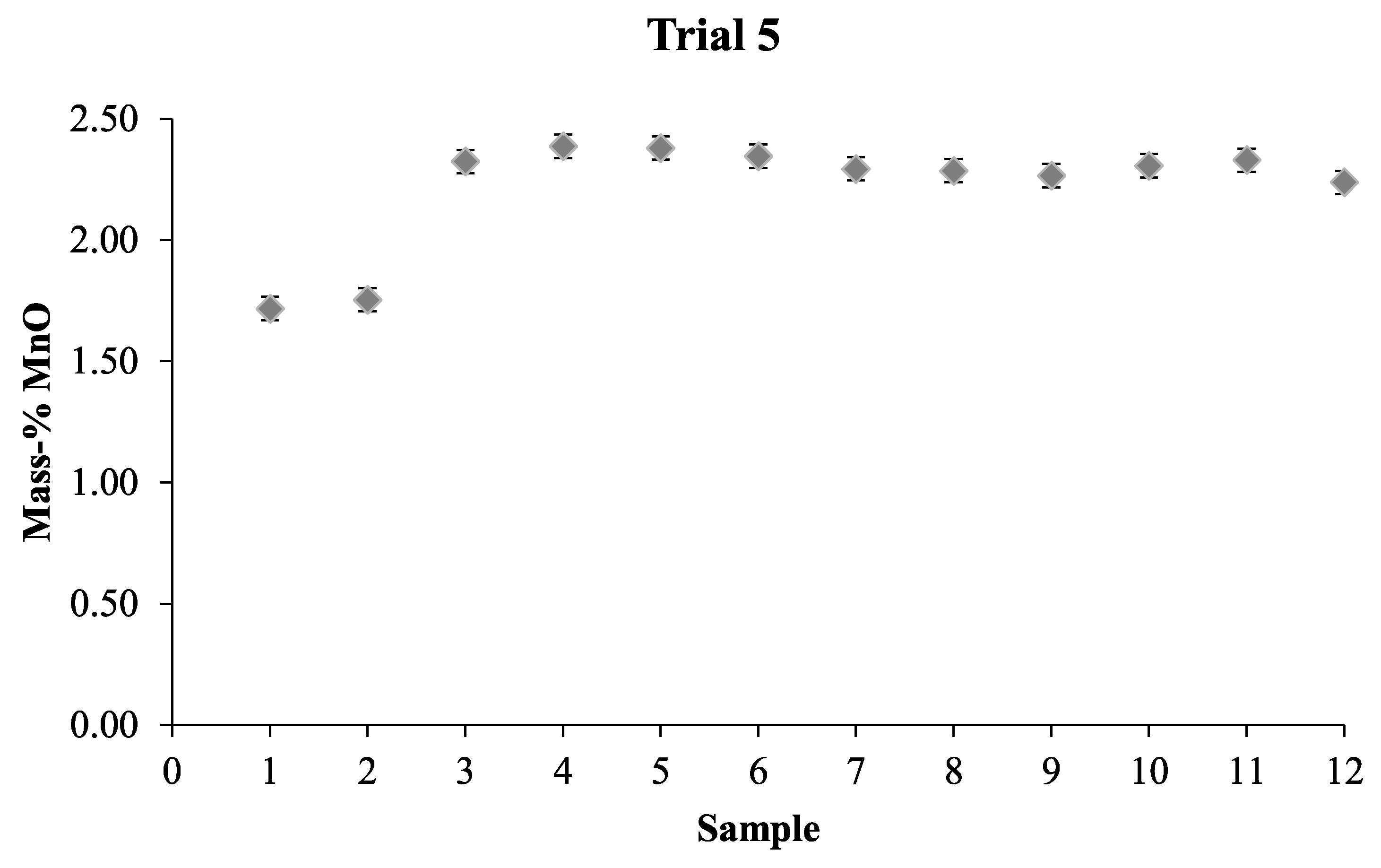
As can be seen in Table 8, the major slag elements were basically the same in each different trial. However, some differences can be seen between the slags. Namely, that the slag in Trials 1 and 2 had more than 54 mass-% FeO while the slag used in Trial 3 only contained 2.5 mass-% FeO. In the slag for Trial 4 there were small amounts of NiO present in the slag and more MnO was present in the slag in Trial 5 compared to the other trials. A low amount of MnO was present in all slags, since it was used as the tracer for the mixing time trials. Therefore, it was only considered for the slag used in Trial 5 when the amount of liquid phase was investigated using the Thermo-Calc calculations, since this slag had the highest amount of MnO.

The database TCOX7 was used for the calculations, as mentioned earlier. All slags with the compositions stated in Table 8 were used. The operating slag temperatures were somewhere around 1200–1600 °C. For all Thermo-Calc calculations, both a closed system and an open system with an oxygen potential with the same value as the surrounding atmosphere were used. The oxygen potential was also varied for the different slags to be able to see the variation in the melting temperatures. 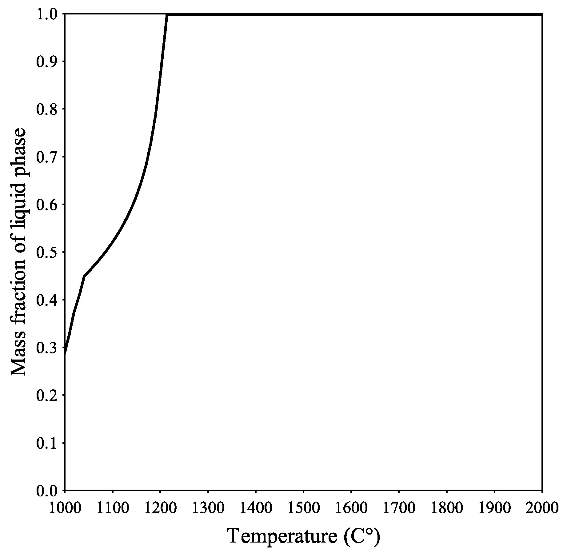The results from the calculations for the slags in Trials 1 and 2 are shown in Figure 7, Figure 8 and Figure 9. These results were selected since they contained the highest amounts of FeO. Therefore, they are most important as the composition was closest to the composition of the future up-scaled IronArc production slag. These calculations were performed for atmospheric pressure. In Figure 7, the results for the closed system are shown. According to the results obtained from the closed system, the slag at 1000 °C had a 30% liquid phase content and was completely melted and in a liquid state at 1250 °C. This is in line with the LOM investigation results that indicate that the slag was in a liquid state at the operating temperature.

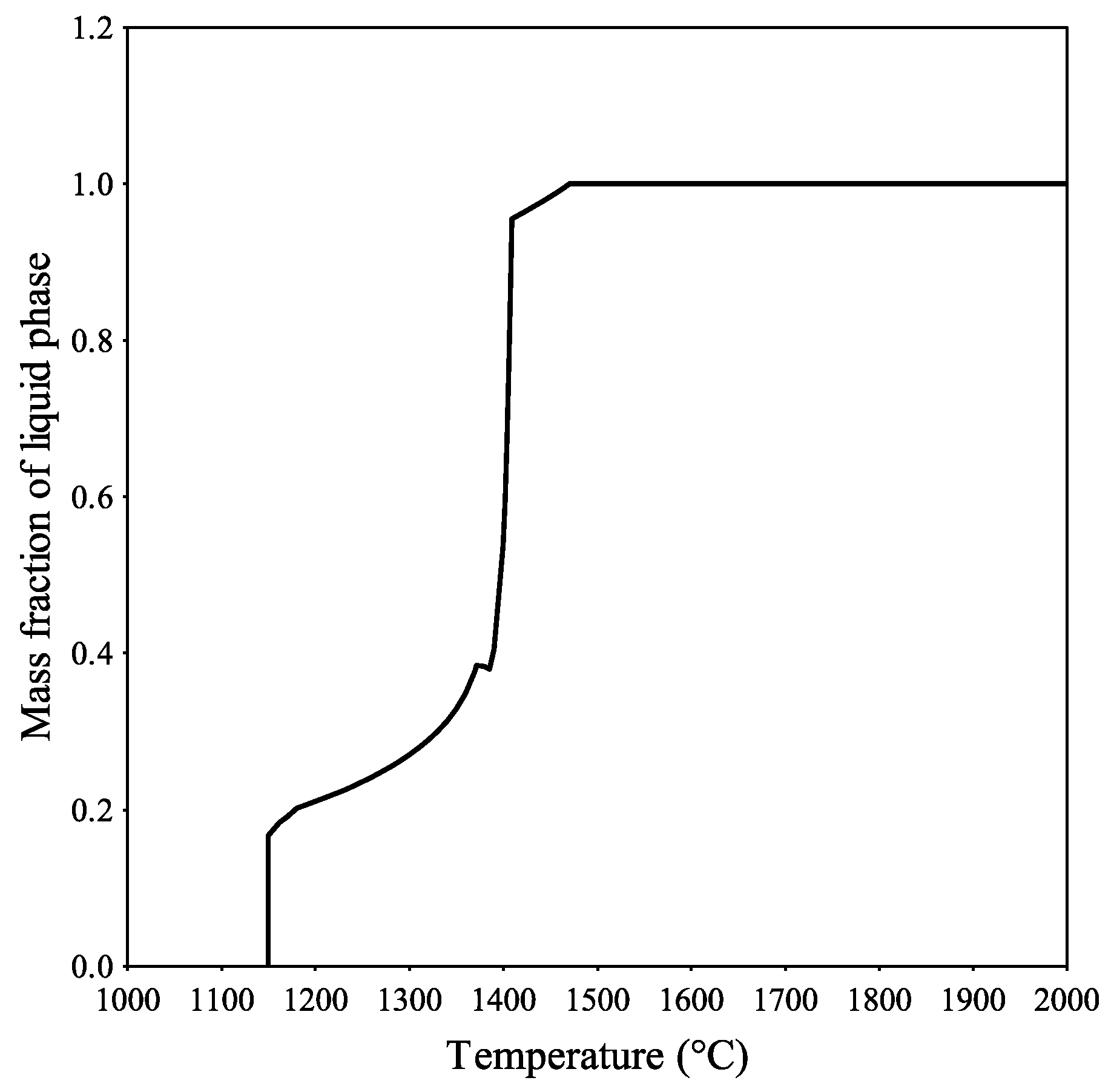
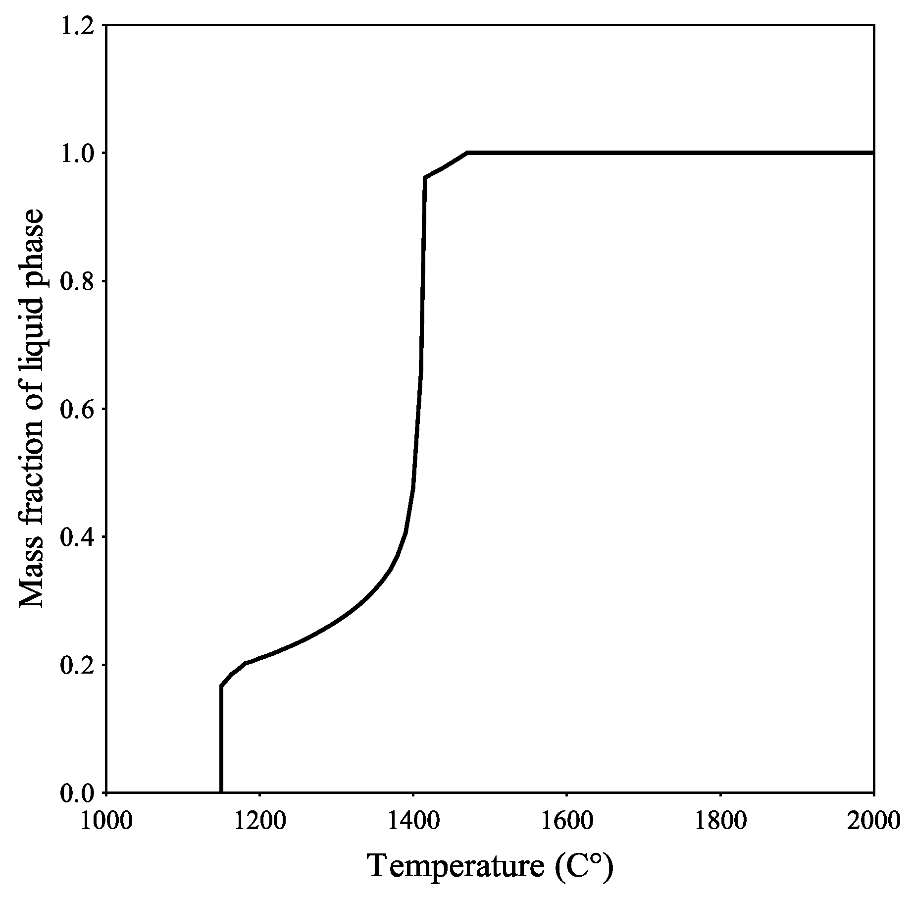
Figure 8 shows the mass fraction of the slag for an open system, where the slag is in equilibrium with an oxygen potential of 0.3. Figure 9 presents a similar calculation, but with an oxygen potential of 0.8. For both cases, the melting started at a higher temperature than given by the closed system and reached a liquid state higher than 90% at 1400 °C and were fully liquid at approximately 1470 °C. When observing the liquids line, the case seems to be that the oxygen potential did not affect the melting temperature to that extent, where the curves and a liquid amount of 95% differs by only 0.4%, when comparing the data for an oxygen potential value of 0.3 and 0.8 (Figure 8 and Figure 9). A completely liquid slag was reached at the same temperature. The larger difference was between an open and closed system, where the melting temperature was 1250 °C and 1450 °C according to the results for the slag elements in Table 8. However, both the results obtained from an open and closed system indicate that the slag was in a liquid state during the operation of the pilot plant reactor. The results for the open system show a melting temperature that is closer to and on the limit of the pilot plant operation conditions. Similar calculations were done for Trials 3 to 5, for a closed system as well as for both higher and lower oxygen potentials. The results for these calculations were similar, but the closed system was closer in melting temperature to the open system compared to the slag used in Trials 1 and 2. In addition, the melting temperatures for these slags were predicted to be approximately 1400 °C. What should be noted is that the total number of elements in the slags is between 20 and 29, which is much higher than the number of elements that is used in the Thermo-Calc calculations. The amounts were reduced to ease the calculations and therefore only the elements with ≥1 mass-% were included. Since the number of elements in the actual slag was several times higher than in the calculations, the melting point should not have been higher than those in the results from the calculations. Often, a higher number of elements means a lower melting point for alloys compared to the pure metals of that alloy. Eutectic alloy systems often offer a lower melting point than the pure elements and also good fluidity [22]. Furthermore, some of the elements that were not included in the calculations were sodium oxides, potassium oxides, and boron oxides. These elements work as fluxes and it is likely that the melting temperature of the slag would be even lower than in the Thermo-Calc calculations [23,24]. This is of interest since these elements are excluded in the Thermo-Calc calculations and therefore the melting point would be lower than the predicted calculation. Hence, the liquid slag conclusion is strengthened. Additionally, previous investigations have shown that for a slag containing Fe, Si, and O as the main elements, whereby they account for 90% of the slag, the main phase is fayalite and has a melting point of 1200 °C [25]. The slags in Trials 1 and 2 also contain the main ion elements Fe, Si, and O, with a combined amount of 90.6 mass-%. This, in turn, gives further indications that the slag will be in a liquid state at the operating temperature of the pilot plant.

When combining the results from the LOM investigation, the mixing time experiments, and the Thermo-Calc calculations, we can assume that the slag in the pilot plant was in liquid state. For future mixing time investigations, it would be beneficial to take samples from different depths and different positions. This would give a clearer picture of the various parts of the bath. Furthermore, with the calculations made on the slag and the results obtained, numerical modeling can now be performed and used to predict the mixing time more accurately as a result of the knowledge that was gained from this investigation.

4. Conclusions

In this work, the mixing time was investigated in the IronArc pilot plant process by performing mixing time experiments in a pilot plant reactor. The mixing, and hence the mixing time, is extremely important in this process. This is because the reduction in the slag bath is dependent on the amount of injected gas, which creates the stirring and homogenization in the liquid slag bath as well as acting as a reduction agent. The mixing time was determined by the addition of a tracer element (MnO₂ powder) and taking continuous samples from the slag. The mixing time was determined as being the time for homogenization of the tracer in the slag. An investigation of the slag phase during operation was also performed by both LOM and Thermo-Calc in order to see if the slag was in liquid state. This would be useful information for future numerical calculations. The following conclusions could be drawn from this work:

• The overall results show that it was possible to approximately determine the mixing time by the addition of a tracer (MnO₂ powder) to the slag. The mixing time for the trials with fast sampling (Trials 3 to 5) showed that the slag was homogenized after just a few seconds. More precisely, for Trial 3, the slag was likely homogenized after 8 s, but definitely after 16 s. The results from Trials 4 and 5 showed the same tendencies, namely that mixing had already been reached in the second samples, 7–8 s after tracer addition.
• The XRF analysis of the MnO content showed a small variation after the final content was reached in the slag for both Trials 1 and 2, which had already been done after the first sample was taken. More specifically, for Trial 1, the MnO content for the samples after addition of tracer varied between 0.41% and 0.43%. Similarly, for Trial 2, the MnO content varied between 0.63% and 0.68%. The standard deviation for Trial 1 was 0.00738 and for Trial 2 it was 0.0165. In addition, the standard errors in both trials were low, namely 0.00233 and 0.00521, respectively. This, in turn, means that there is a relatively small spread in the sampling distribution, indicating that it was possible to get an accurate measurement of the tracer content in the slag.
• The results from the comparison between the theoretical amount of MnO₂ in the slag and the measured value showed that there is quite a large difference. Specifically, the theoretical amount of slag is 27% larger than the measured value. The most probable reason for this difference is that some of the powder was lost through the off-gas pipe before the powder entered the slag.
• It was seen in the LOM investigation that the microstructure was clearly dependent on the cooling speed. The finest structure was found in the area that had the fastest cooling speed and further into the sample, where it had cooled slower, had a coarser structure. No individual particles that were not part of the solidification could be seen in the microstructure. Thus, it can be concluded that the large majority of the slag was in a liquid state before it was cooled.
• A phase analysis in the Thermo-Calc software showed that a large majority of the slag, or the entire slag, was in liquid state at the operating temperature. Just a fraction of the number of elements were used in the calculations. Therefore, the actual number of elements is much larger. This, in turn, means that the melting point should have been even lower than what the calculations suggested. To summarize, taking into account this and the LOM investigation, it can be concluded that the slag was in a liquid state during the operational conditions.

References

1. ScanArc Plasma Technologies AB. Järnreduktionsprocess Och Anordning Därför. U.S. Patent No. SE1250215A, 8 March 2013. [Google Scholar]
2. Bölke, K.; Ersson, M.; Ni, P.; Swartling, M.; Jönsson, P.G. Physical Modeling Study on the Mixing in the New IronArc Process. Steel Res. Int. 2018, 89, 1–10. [Google Scholar] [CrossRef]
3. Bölke, K.; Ersson, M.; Imris, M.; Jönsson, P.G. Importance of the Penetration Depth and Mixing in the IRONARC Process. ISIJ Int. 2018, 58, 1210–1217. [Google Scholar] [CrossRef]
4. Zhou, X.; Ersson, M.; Zhong, L.; Yu, J.; Jönsson, P.G. Mathematical and Physical Simulation of a Top Blown Converter. Steel Res. Int. 2014, 85, 273–281. [Google Scholar] [CrossRef]
5. Zhou, X.; Ersson, M.; Zhong, L.; Yu, J.; Jönsson, P.G. Optimazation of Combined Blown Converter Process. ISIJ Int. 2014, 54, 2255–2262. [Google Scholar] [CrossRef]
6. Zhou, X.; Ersson, M.; Zhong, L.; Yu, J.; Jönsson, P.G. Numerical and Physical Simulations of a Combined Top-Bottom-Side Blown Converter. Steel Res. Int. 2015, 86, 1328–1338. [Google Scholar] [CrossRef]
7. Visuri, V.; Isohookana, E.; Kärnä, A.; Haas, T.; Eriç, R.H.; Fabritius, T. A physical modelling study of mixing in an AOD vessel. In Proceedings of the 5th International Conference on Process Development in Iron and Steelmaking, Luleå, Sweden, 12–15 June 2016. [Google Scholar]
8. Wupperman, C.; Giesselmann, N.; Rückert, A.; Pfeifer, H.; Odenthal, H. A Novel Approach to Determine the Mixing Time in a Water Model of an AOD Converter. ISIJ Int. 2012, 52, 1817–1823. [Google Scholar] [CrossRef] [Green Version]
9. Samuelsson, P.; Ternstedt, P.; Tilliander, A.; Apell, A.; Jönsson, P.G. Use of physical modelling study how to increase the production capacity by implementing a novel oblong AOD converter. Ironmak. Steelmak. 2018, 45, 335–341. [Google Scholar] [CrossRef]
10. Ternstedt, P.; Tilliander, A.; Jönsson, P.G.; Iguchi, M. Mixing Time in a Side-Blown Converter. ISIJ Int. 2010, 50, 663–667. [Google Scholar] [CrossRef] [Green Version]
11. Wei, J.H.; Ma, J.C.; Fan, Y.Y.; Yu, N.W.; Yang, S.L.; Xiang, S.H.; Zhu, D.P. Water modelling study of fluid flow and mixing characteristics in bath during AOD process. Ironmak. Steelmak. 1999, 26, 363–371. [Google Scholar] [CrossRef]
12. Wei, J.H.; Yu, N.W.; Fan, Y.Y.; Yang, S.L.; Ma, J.C.; Zhu, D.P. Study on flow and mixing characteristics of molten steel in RH and RH-KTB refining prosesses. J. Shanghai Univ. 2002, 6, 167–175. [Google Scholar] [CrossRef]
13. Fabritius, T.M.J.; Mure, P.T.; Harkki, J.J. The Determination of the Minimum and Operational Gas Flow Rates for Sidewall Blowing in the AOD-Converter. ISIJ Int. 2003, 43, 1177–1184. [Google Scholar] [CrossRef] [Green Version]
14. Odenthal, H.J.; Thiedemann, U.; Falkenreck, U.; Schlueter, J. Simulation of Fluid Flow and Oscillation of the Argon Oxygen Decarburization (AOD) Process. Metall. Trans. B 2010, 41, 396–413. [Google Scholar] [CrossRef]
15. Fabritius, T.M.J.; Kupari, P.A.; Harkki, J.J. Physical modelling of a sidewall-blowing converter. Scand. J. Metal. 2001, 30, 57–64. [Google Scholar] [CrossRef]
16. Kasban, H.; Zahran, O.; Arafa, H.; El-Kordy, M.; Elaraby, S.M.S.; Abd, F.E. Laboratory experiments and modeling for industrial radiotracer applications. Appl. Radiat. Isot. 2010, 68, 1049–1056. [Google Scholar] [CrossRef] [PubMed]
17. Othman, N.; Kamarudin, S.K. Radiotracer Technology in Mixing Processes for Industrial Applications. Sci. World J. 2014, 2014, 1–15. [Google Scholar] [CrossRef] [PubMed]
18. Perry, D.L. Handbook of Inorganic Compounds, 2nd ed.; CRC Press: Boca Raton, FL, USA, 2011; p. 267. [Google Scholar]
19. Fujii, Y.; Nakai, Y.; Uchida, Y.; Miki, Y. Fundamental investigation of high temperature reduction and melting behavior of manganese ore. ISIJ Int. 2017, 57, 609–614. [Google Scholar] [CrossRef]
20. Andersson, J.O.; Helander, T.; Höglund, L.; Shi, P.; Sundman, B. Thermo-Calc & DICTRA, computational tools for materials science. Calphad 2002, 26, 273–312. [Google Scholar]
21. TCOX7 (TCS Metal Oxide Solutions Database), version 7; Thermo-Calc Software AB: Solna, Sweden, 1992.
22. Morando, C.; Fornaro, O.; Garbellini, O.; Palacio, H. Fluidity on Metallic Eutectic Alloys. Procedia Mater. Sci. 2015, 8, 959–967. [Google Scholar] [CrossRef] [Green Version]
23. Hasanuzzaman, M.; Rafferty, A.; Sajja, M.; Olabi, A.-G. Production and Treatment of Porous Glass Materials for Advanced Usage. In Reference Module in Materials Science and Materials Engineering; Elsevier: New York, NY, USA, 2016; pp. 1–11. [Google Scholar]
24. Britt, J. The Complete Guide to High-Fire Glazes; Sterling Publishing Co., Inc.: New York, NY, USA, 2004; pp. 18–19. [Google Scholar]
25. Cheng, X.; Zhao, K.; Qi, Y.; Shi, X.; Zhen, C. Direct Reduction Experiment on Iron-Bearing Waste Slag. J. Iron Steel Res. Int. 2013, 20, 24–29. [Google Scholar] [CrossRef]
Figure 1. Schematic picture of the sampling procedure with the addition of tracer and sampling rod.
Metals 09 00101 g001
Figure 2. Content MnO (%) for the different samples for Trial 1 and Trial 2, respectively. The MnO2 powder was added after sample 2 for Trial 1 and after sample 15 for Trial 2.
Metals 09 00101 g002
Figure 3. Content of MnO (%) for all the samples taken during Trial 3, where samples 1 and 2 were taken before tracer addition and the rest of the samples were taken after the addition of the MnO2 tracer powder.
Metals 09 00101 g003
Figure 4. Content of MnO (%) for all the samples taken during Trial 4, where samples 1 and 2 were taken before tracer addition and the rest of the samples were taken after tracer addition.
Metals 09 00101 g004
Figure 5. The amount of MnO (%) in each slag sample taken during the pilot plant experiment.
Metals 09 00101 g005
Figure 6. Light optic microscope (LOM) picture of 2D cross-section surface of slag sample. The numbers represent different zones in the sample.
Metals 09 00101 g006
Figure 7. The mass fraction of liquid phase for the slags used in Trials 1 and 2 for a temperature span between 1000 and 2000 °C. The calculations were made for a closed system.
Metals 09 00101 g007
Figure 8. The mass fraction of liquid phase in the slags used in Trials 1 and 2 for a temperature span between 1000 and 2000 °C. The calculations were done by assuming an open system with an oxygen potential of 0.3.
Metals 09 00101 g008
Figure 9. The mass fraction of liquid phase in the slags used in Trials 1 and 2 for a temperature span between 1000 and 2000 °C. The calculations were done by assuming an open system with an oxygen potential of 0.8.
Metals 09 00101 g009