On the Use of JMAK Theory to Describe Mechanical Amorphization: A Comparison between Experiments, Numerical Solutions and Simulations

Abstract

The kinetics of amorphization during ball milling is generally analyzed using two different approaches: the classical Johnson-Mehl-Avrami-Kolmogorov (JMAK) theory and Delogu and Cocco’s model for which a region deterministically transforms after it reaches a certain number of collisions. The application of JMAK analysis to the latter model predicts Avrami exponents to be higher than the experimental ones (typically close to one). We develop simulations based on the probabilistic character of the nucleation phenomenon and concave growth of the amorphous phase in the core of a nanocrystal. The predictions of our simulations are in good agreement with the low Avrami exponents and with the size evolution of the remaining crystallites found experimentally. From these values, the parameters involved in the simulated model (growth rate and probability of nucleation) can be estimated.

1. Introduction

The development of amorphous alloys in the 1960s by Paul Duwez [1] opened a new branch of research about the properties, microstructures and kinetics of these metastable systems [2,3]. Rapid quenching is the standard method used to achieve an amorphous structure in which a strongly disordered, high temperature, liquid-like structure is frozen. However, in the early 1980s, some authors [4,5] discovered the viability of producing amorphous alloys after mechanical processing by milling. Since then, the production of amorphous systems via mechanical alloying and/or milling (in a much broader compositional range than that obtained by rapid quenching methods [6]) has been widely found in the literature [2].

It is evident that the mechanisms that induce amorphization from mechanical milling are completely different to those that preserve the liquid-like structure by rapid quenching. However, different microstructural and thermal analyses have shown equivalent behaviors of the obtained amorphous structures (e.g., glass transition temperature, amorphous halo observed by diffraction techniques, etc.) [2,3,7,8].

Although the amorphization of some alloys by high energy milling has been known since the early 1980s, the kinetics describing this process are still under discussion. Schwarz and Johnson [9] reported some required conditions to obtain amorphous alloys in solid state reactions at low temperatures in transition metal binary systems. However, the process of amorphization by ball milling has been widely reported in systems that do not fulfil those conditions [5,10]. From this, notable advances in the field have been achieved with theoretical and numerical investigations [11,12,13,14]. Some reviews on ball milling found in the literature also describe the different attempts to characterize the thermodynamics of amorphization via milling [2] and summarize the literature on transformation kinetics during milling [3]. Direct application of the classical theory developed by Kolmogorov [15], Johnson and Mehl [16] and Avrami [17] (JMAK), which takes into account the nucleation and growth processes, has been reported along with phenomenological exponential laws [18], which can be interpreted based on the probability of powder particles of being trapped between colliding balls and walls [19]. Despite the experimental values of Avrami exponents reported in the literature, mechanical amorphization is not expected to satisfy the conditions of the JMAK theory. In fact, in order to be described by JMAK theory, mechanical amorphization must satisfy the five postulates of Kolmogorov [20]:

• The initial parent phase is progressively and completely replaced by a product phase;
• The volume of any transformed region is tiny with respect to the whole volume of the system;
• Nucleation is random;
• The shape of the growing phase is convex;
• The linear growth rate can be expressed as a product of a time-dependent function and a direction-dependent function.

Although postulates 1, 2 and 5 can be considered valid for mechanical transformation processes, postulates 3 and 4 cannot. In particular, the growth of the new phases as convex regions is not supported by transmission electron images (see, for example, [21]) that have shown the remnant nanocrystals to have regular shapes during the amorphization process. Moreover, nucleation is not random, as boundary regions between nanocrystals are expected to be the nucleation sites of the amorphous phase.

Even though the JMAK model should not be applicable to mechanical amorphization, the easy and well-established procedure to extract average kinetics parameters in this frame makes it attractive to kinetics researchers. In fact, an analysis based on JMAK can easily supply kinetics information (Avrami exponent and frequency constant) that can be compared with already-published values. Therefore, understanding the actual meaning of the kinetics parameters obtained from JMAK under the framework of a more realistic model should be welcomed. This is one of the aims of the present paper.

Concerning the transformation kinetics during milling, Delogu and Cocco [22] developed a general model (D&C model) to describe different mechanical transformations based on the assumption that individual collisions deterministically induce finite local transformations in small volumes. Within such volumes, mechanical stresses are assumed to be able to activate a transformation within a short time interval. According to this statistical framework, the amorphization process starts when the powders have experienced a certain number of critical loading events, which depends on the impact energy. Typically, amorphization processes require tens of hours [5,23], which corresponds to millions of collisions [24].

In the present paper, the applicability of the JMAK and D&C approaches to describe mechanical amorphization is discussed. Moreover, a third model is developed here, which assumes that the nucleation has a probabilistic character and that the interface-controlled growth affecting the particles trapped in a collision has a deterministic character. The predictions of the different models are compared to the results from experiments, numerical solutions and simulations based on the third model. An effective JMAK analysis is used to compare the different models. The key point of the present work is thus the description of a new physical framework that is consistent with microstructural and kinetic experimental results. In order to compare this new framework with previously used ones (JMAK and D&C) we build JMAK plots to extract the effective JMAK parameters which are widely available in the literature.

2. Materials and Methods

In order to test the predictions of the different models here described, besides literature data, two binary compositions, Fe₇₀Zr₃₀ and Fe₇₀Nb₃₀, were prepared from mechanical alloying by ball milling in a planetary mill Fritsch Pulverrisette 4 Vario (Fritsch GmbH, Idar-Oberstein, Germany) from elemental powders (>99%). The initial powder mass was 30 g, and the ball to powder ratio was 10:1. The disc frequency was set at 350 rpm, and the frequency ratio was set at −2. Milling was performed in 30 min steps, followed by 30 min pauses. Under these conditions, the temperature rise inside the vial was about 10 K [25].

The evolution of the amorphous phase with milling time was estimated from the fractional area of the paramagnetic site contributions to the total Mössbauer spectra (MS) (WissEl Wissenschaftliche Elektronik GmbH, Starnberg, Germany). This technique is clearly more sensitive than X-ray diffraction (XRD) for detecting small fractions of paramagnetic phases in a ferromagnetic matrix and vice versa [26]. The sizes of the remaining crystals were estimated from the area ratio of the interface and core contributions to MS [27]. Numerical solutions and simulations were performed using Matlab scripts (Matlab R2016a, The Mathworks Inc., Natick, MA, USA).

3. Results and Discussion

3.1. Mechanical Amorphization Described by JMAK Theory

The JMAK theory uses the concept of the extended transformed fraction, X*. This parameter corresponds to the expected transformed fraction without taking into account the overlapping between different growing regions. Therefore, simple assumptions about the nucleation and growth mechanisms yield [28]:

$$X^{*}={\left(k\left(t-t_0\right)\right)}^n,$$

(1)

where t₀ is the induction time, k is a frequency factor, and n is the Avrami exponent. The latter parameter is related to the nucleation and growth mechanisms, i.e., n = n_I + d·n_G, where n_I = 1 for a constant nucleation rate and 0 for the absence of nucleation, d is the dimension of growth, and n_G = 1/2 for diffusion-controlled growth and 1 for interface-controlled growth [28]. Finally, X* is statistically related to the actual transformed fraction (amorphous fraction, in our case, X_Am) as:

$$\frac{d{X}_{Am}}{d{X}^{*}}=1-X_{Am}.$$

(2)

From these two equations, the well-known JMAK equation is obtained:

$$X_{Am}=1-e^{-{\left(k\left(t-t_0\right)\right)}^n}.$$

(3)

Using Equation (3), a plot of ln[−ln(1 − X_Am)] vs ln(t − t₀) (JMAK plot) allows us to obtain the values of n (from the slope) and k (from the intercept) after a fitting to a straight line.

The JMAK theory, developed for thermally-induced isothermal transformations, requires that nuclei grow in a convex way (i.e., fulfilling the forth postulate of Kolmogorov [20]). However, it would be rather more feasible for the nucleation of the amorphous phase during mechanical amorphization to occur at the boundaries between nanocrystals. These regions are already in a disordered configuration due to the high defect concentrations in these regions induced by the milling treatment. The way to store higher amounts of mechanical energy in these systems should be to increase the thickness of the interface layer, as the nanocrystals are too small to incorporate crystalline defects such as dislocations (which have been only observed under extremely high pressures [29]). From these boundaries, the nanometric crystallites should be reduced and thus, the growing front must be concave [26], unlike that required by the JMAK theory. However, although the application of the JMAK theory to mechanical amorphization should be inappropriate for general cases. For those in which the transformation of the nanocrystal to amorphous occurs very fast, the growing mechanism can be neglected, and then Equation (3) can be simplified for the case n = 1:

$$X_{Am}=1-e^{-k\left(t-t_0\right)}.$$

(4)

In fact, the Avrami exponents found in the literature are close to 1 [30,31,32,33,34,35,36]. Therefore, in the frame of JMAK theory, mechanical amorphization should have very fast growth transformation (n = n_I, with 1 representing a constant nucleation rate), so that the information obtained from the analysis is then limited to the frequency parameter, k, which is equivalent to the probability of nucleation per unit of time.

From Equation (4), the transformation rate can be obtained from:

$$\frac{d{X}_{Am}}{dt}=k{e}^{-k\left(t - t_0\right)}=k\left(1 - X_{Am}\right),$$

(5)

Figure 1 shows the transformed fraction and the transformation rate for a JMAK system with n = 1 (i.e., described by Equations (4) and (5), respectively). It can be observed that the transformation rate continuously decreases and there is no maximum at times other than zero. It will be shown in the next sections that this is not an appropriate description of the experimental data.

Explanation for Effective Avrami Exponents Below 1

The Avrami exponents reported for mechanical amorphization in the literature are close to one but, in many cases, values lower than 1 have been found. This can be understood by taking into account some artifacts that can affect any JMAK analysis, namely, indeterminations in the induction time and the normalization of X_Am. Moreover, the presence of a non-zero amorphous fraction at the starting point can also produce artificially lower effective Avrami exponents, n_eff.

In order to study the effect of these artifacts, we generated X_Am curves using the JMAK equation and a zero-induction time. These curves were analyzed using JMAK plots assuming different erroneous induction times or factors leading to the underestimation or overestimation of the transformed fraction. Figure 2 (upper panel) shows the effect of indetermination on the induction time in the JMAK plot for the case of n = 1. The effective Avrami exponent decreases and linearity gets worse as the overestimation of the induction time increases. The lower panel of Figure 2 shows the effect of a non-correct estimation of the transformed fraction. The underestimation of the transformed fraction also reduces n_eff. Strong deviations can yield an artificial two-slope behavior.

Besides these two artifacts, when dealing with JMAK analyses, the presence of a starting non-zero transformed fraction is also worthy of a brief analysis under the framework of mechanical amorphization. In fact, considering that the amorphous phase has its origin at the crystal boundaries [26], it is plausible to assume a starting fraction (a layer) of amorphous phase, X₀ ≠ 0, is present. In this case, the extended fraction should be:

$${X_{Am}}^{*}={\left(kt+{X_0}^{*}\right)}^n,$$

(6)

with X₀* = −ln(1 − X₀). Therefore, the transformed fraction would be:

$$X_{Am}=1-e^{-{\left(kt - {X_0}^{*}\right)}^n},$$

(7)

We generated different curves using Equation (7) with different values of X₀, and n = 1 and t₀ = 0. These curves were analyzed without considering a zero-starting fraction, i.e., using the conventional JMAK plot. The n_eff and effective frequency factor, k_eff, values are shown in Figure 3 as functions of X₀. As an example, n_eff~0.8 for X₀~0.15. For typical nanocrystal size of ~10 nm, this starting value will require an initial amorphous thickness of ~0.25 nm, which is approximately the atomic distance and thus, is too small to be detected. Such a small value is typical for coherent crystal boundary regions. Therefore, thicker boundaries, expected to be the nucleation sites of the amorphous phase, may have an even larger effect. This implies that difficulties in the early detection of transformation yield lower n_eff values than the actual values. In the case of k_eff, this parameter linearly increases with X₀ (e.g., for X₀ = 0.2, k_eff~1.25 k).

3.2. Mechanical Amorphization Described by the Number of Collisions

Delogu and Cocco [22] developed a general model (D&C model) to describe the different processes occurring during ball milling, ascribing the progress of transformation to the number of collisions. The transformation of a certain region is assumed to occur after this region achieves a certain number of collisions (i.e., a deterministic character is assumed for the transformation). The probability of a region accumulating the required number of collisions is determined by the fraction of a sample trapped in a collision (this probability jeopardizes the deterministic character assumed for the nucleation). The authors supplied the following expression for the fraction of the system involved in j collisions after q collisions occur in the mill [22]:

$$X_{Am}=1-e^{-k_{col}q}\left(1+{{\displaystyle \sum }}_{i=2}^j\frac{{\left(k_{col}q\right)}^{i-1}}{\left(i-1\right)!}\right) ,$$

(8)

where k_col is the fraction of the sample affected per collision, and q is the total number of collisions. Due to the periodic character of the dynamics involved in ball milling (either vibrating [37], shaking [38] or planetary mills [39]), the total number of collisions (q) can be determined by the milling time (t), and the k_col to k’ fraction of powder affected per unit time. Therefore, Equation (8) can be rewritten to represent the amorphous fraction as a function of the milling time:

$$X_{Am}=1-e^{-k^{\prime }t}\left(1+{{\displaystyle \sum }}_{i=2}^j\frac{{\left(k^{\prime }t\right)}^{i-1}}{\left(i-1\right)!}\right) .$$

(9)

The derivative of this expression can be obtained by considering the number of new regions activated in an interval, dτ:

$$\frac{d{X}_{Am}}{d\tau }=k^{\prime }{e}^{-k^{\prime }\tau }\frac{{\left(k^{\prime }\tau \right)}^{j-1}}{\left(j-1\right)!} .$$

(10)

The D&C model assumes a further approximation, in which the transformation is considered to occur after a single event [22]. Thus, the particularizing Equation (9) for j = 1 leads to:

$$X_{am}\left(t\right)=1-e^{-k^{\prime }t},$$

(11)

which is equivalent to the JMAK equation with n = 1 and t₀ = 0 (see Equation (4)). Under this framework, the frequency parameter, k’, is identified as the fraction of sample involved in collisions per unit time.

For general cases, we numerically solved Equations (9) and (10) for different values of parameter j. The results are shown in Figure 4.

Except for the case where j = 1, an inflexion point at a time, t_max, exists in the X_Am(t) curves. From the derivative of Equation (10), we can estimate the time taken to reach the maximum rate of transformation (i.e., the inflexion point of X_Am(t)):

$$t_{max}=\frac{j-1}{k^{\prime }}.$$

(12)

Therefore, values of t_max linearly increase with parameter j and the inverse of the frequency, k’.

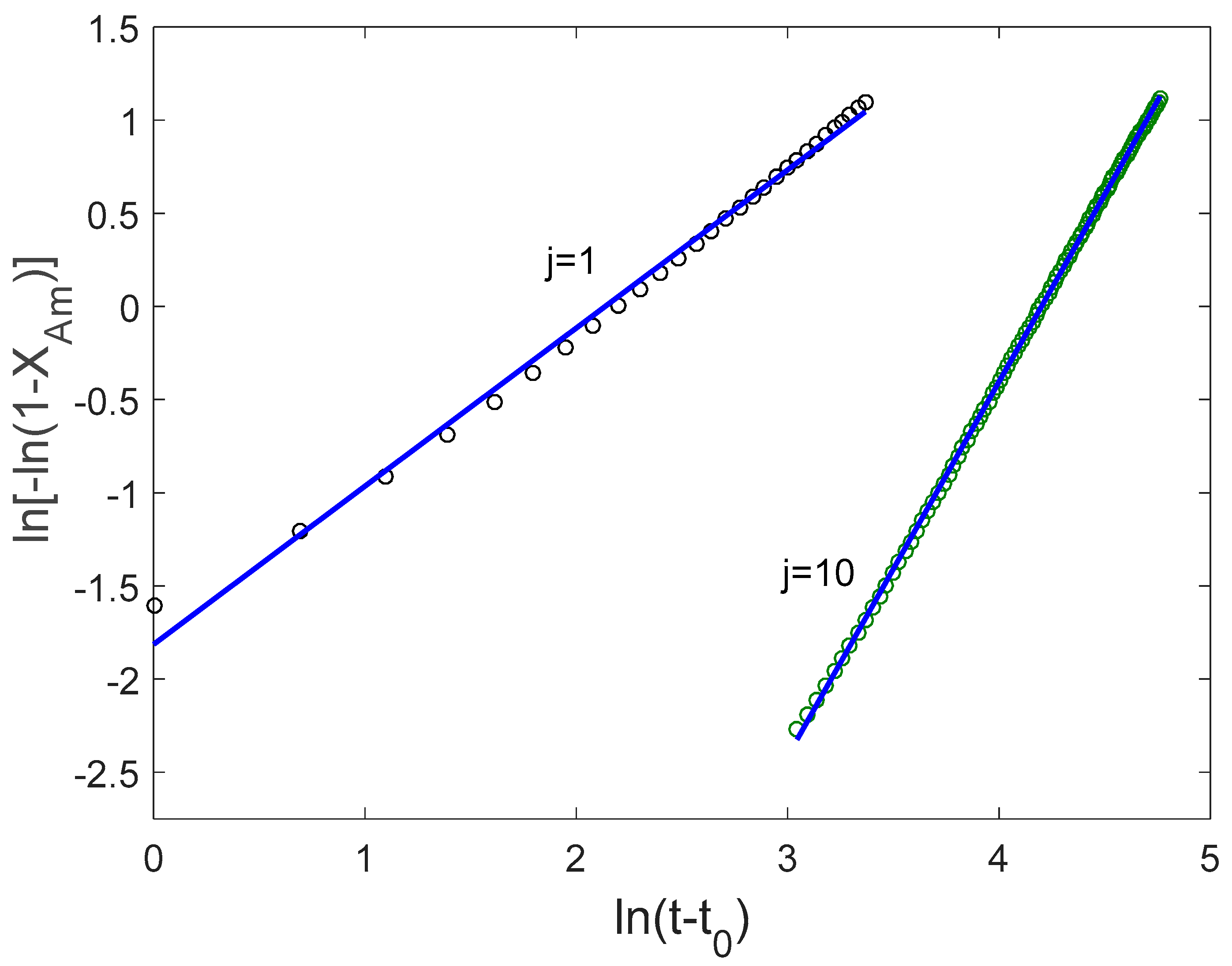
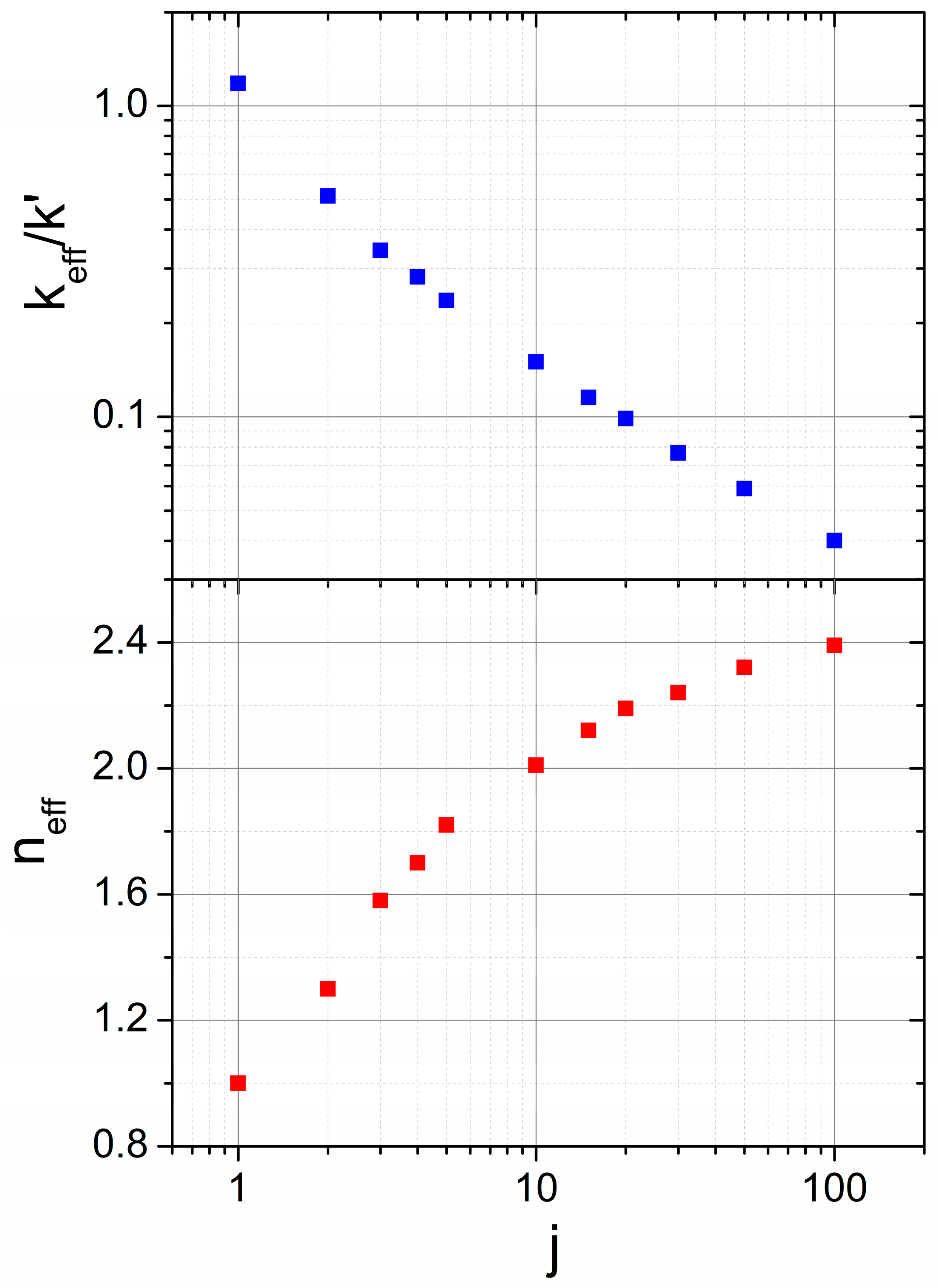
Application of the JMAK Analysis to Delogu and Cocco’s Model

In order to compare the results predicted from the D&C and JMAK models, we built an effective JMAK plot with the numerically generated solutions obtained using Equation (9). To do so, we considered the induction time, t₀, for each X_Am(t) curve to be the time needed to reach X_Am = 0.01. Then, it was possible to plot ln[−ln(1 − X_Am)] vs ln(t − t₀), as shown in Figure 5. A good linearity was observed, and effective values of the Avrami exponent, n_eff, and the frequency factor, k_eff, were obtained (Figure 6). From a practical point of view, data from X_Am = 0.1 to 0.95 were represented. In fact, as described earlier in this text, the determination of the induction time and the completion of the transformation strongly affect results for very low and very high X_Am values, respectively.

As shown in Figure 6, a minimum Avrami exponent, n_eff = 1, was obtained for j = 1 when the model was equivalent to the JMAK model and k_eff = k’. The easy interpretation for this particular case is lost for j > 1. On one hand, k_eff decreases from k_eff~k’ for j = 1 to ~4·10⁻²k’ for j = 100. On the other hand, n_eff continuously increases from n_eff~1 for j = 1 to ~2.4 for j = 100. Therefore, taking into account the Avrami exponents reported in the literature, the general D&C model should be valid for describing mechanical amorphization only when j = 1, which implies a deterministic and sudden change in the regions after the very first collision they are involved in.

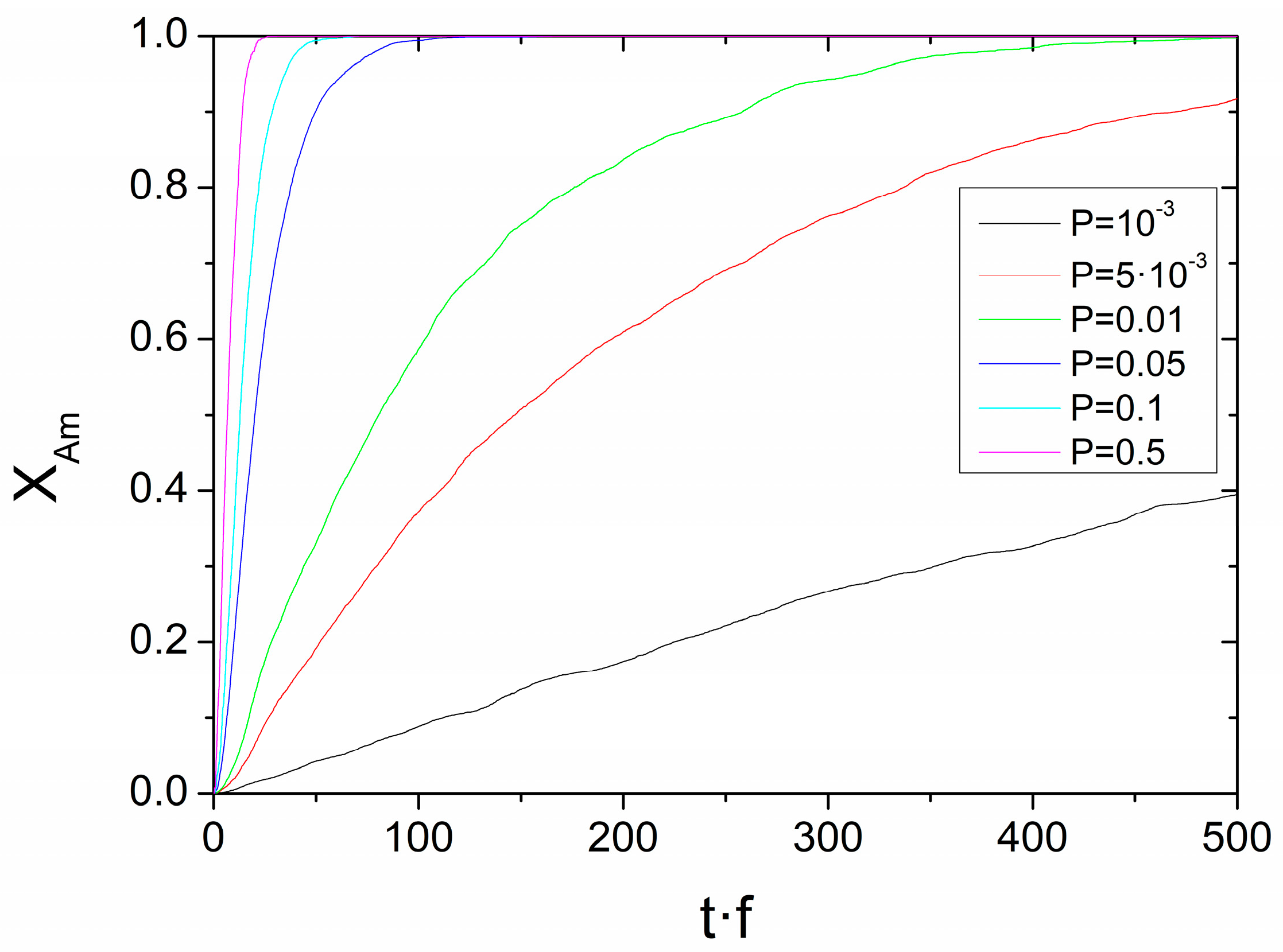
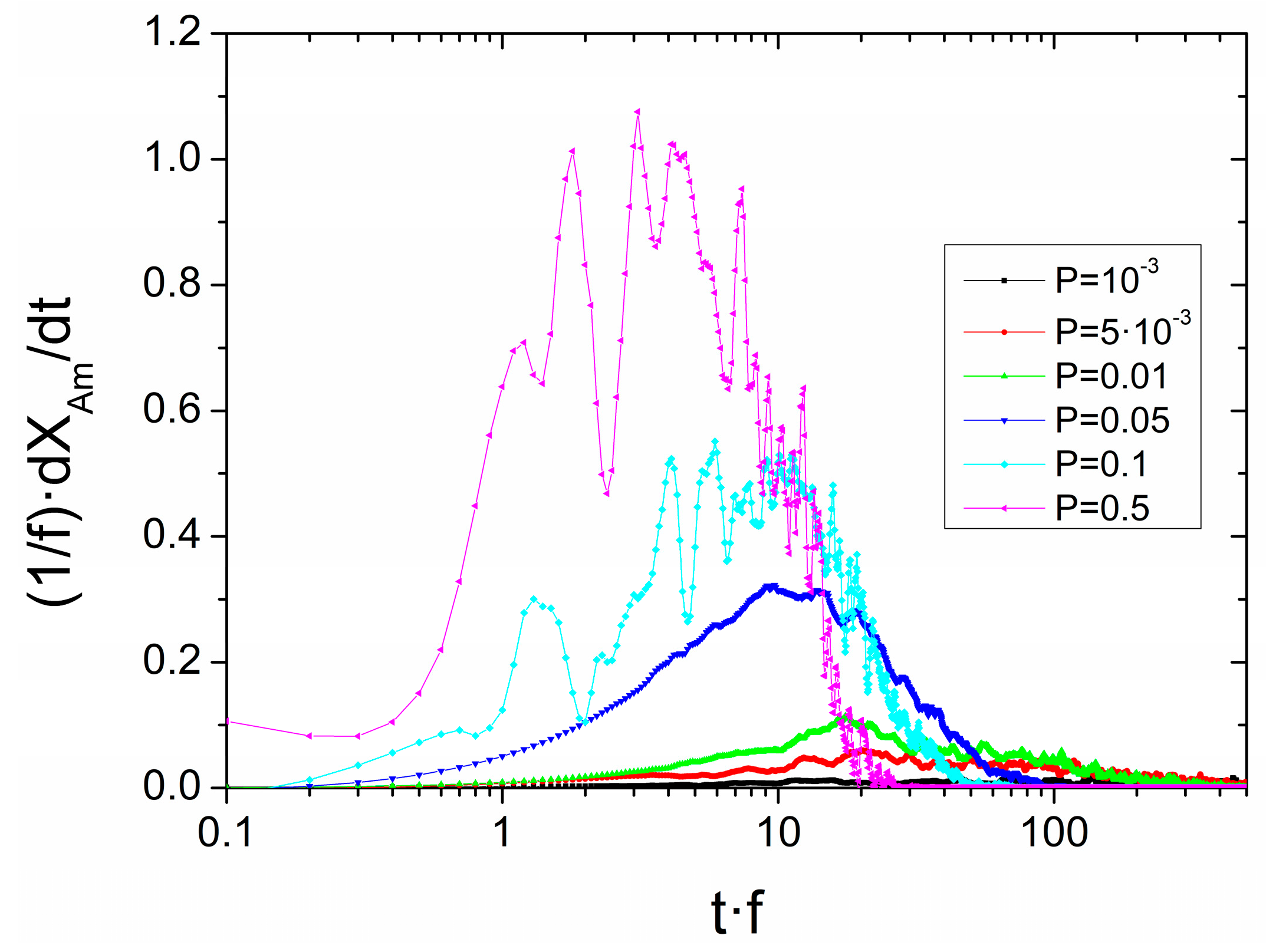
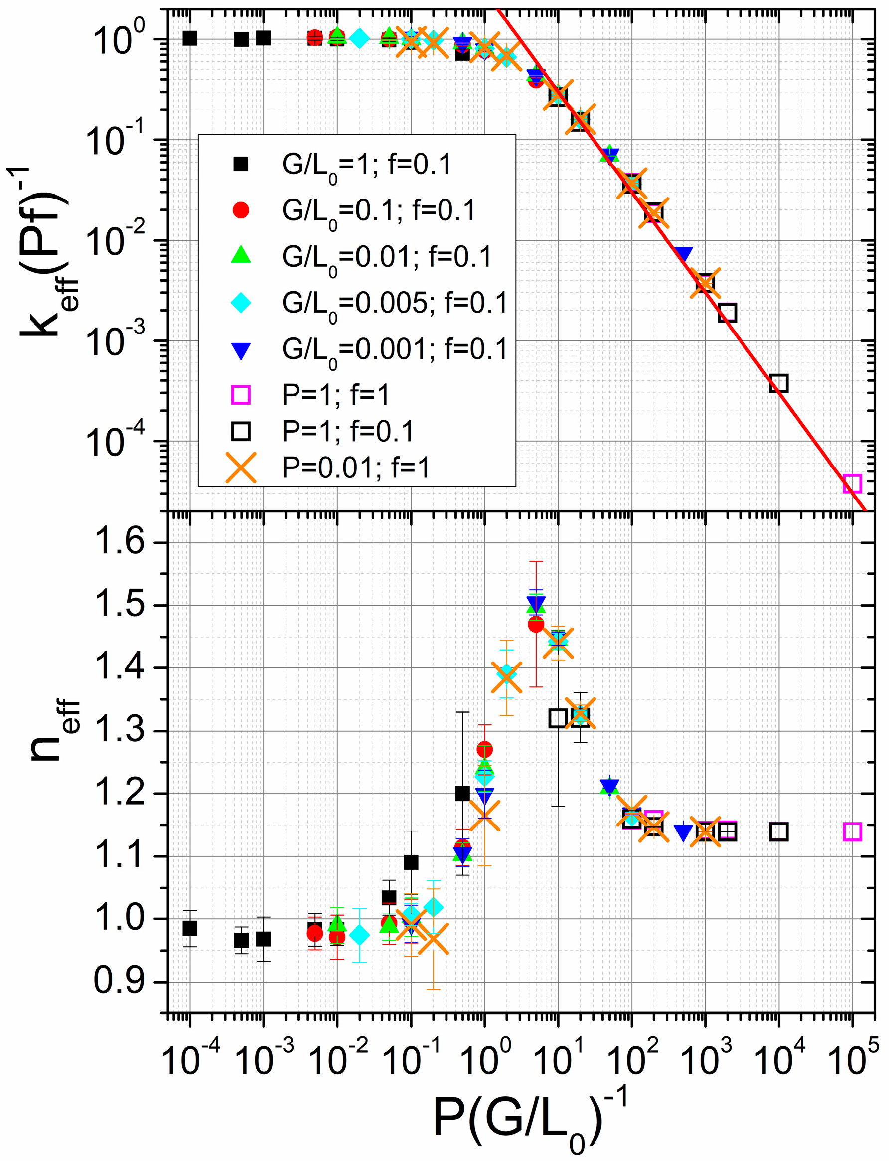
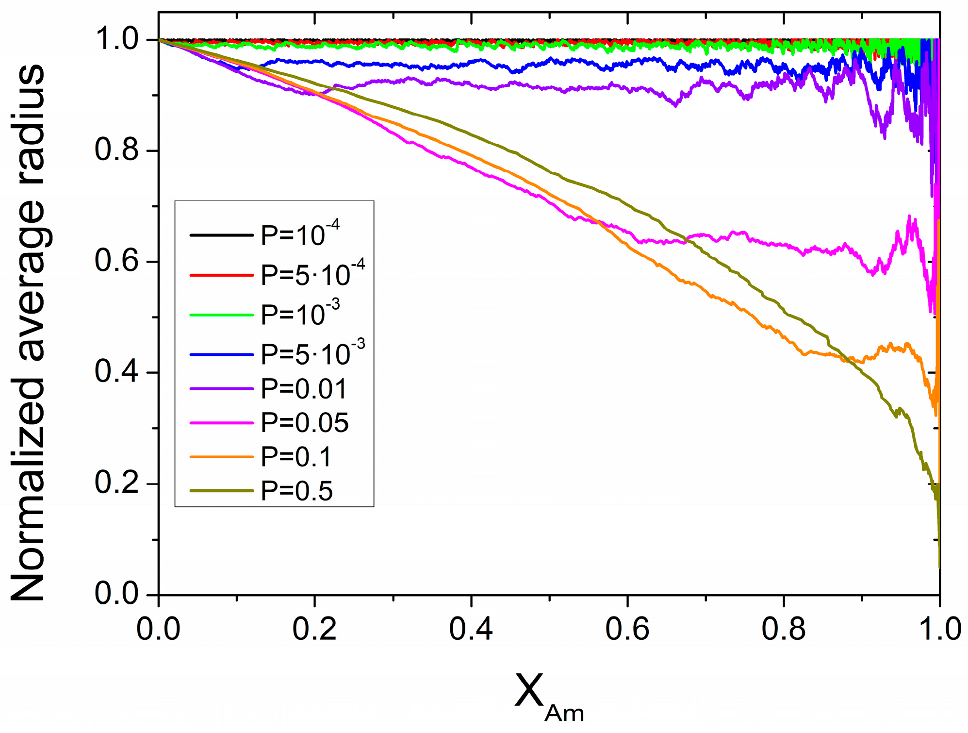
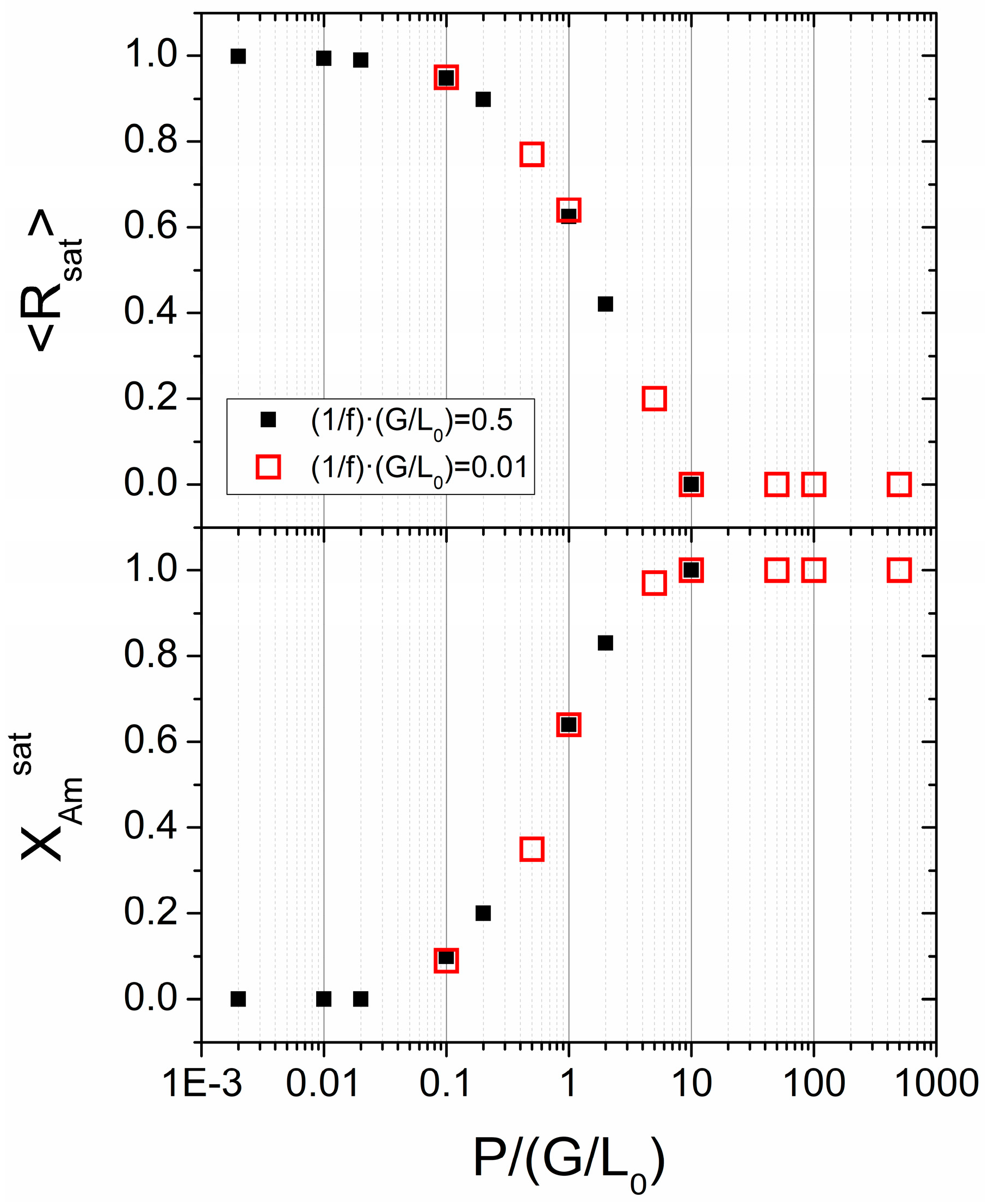
3.3. Simulations Based on a Probabilistic Activation of the Amorphization Process

The D&C model uses a deterministic interpretation of the nucleation process as this will occur after the region accumulates a specific number of collisions. However, the nucleation process is a probabilistic phenomenon [20]. With this idea in mind, we analyzed the behavior of a simulated system consisting of a certain number of spherical crystalline particles, N, initially with a radius, L₀. For every iteration step of the simulation (time is measured in steps units), a fraction, f (units: steps⁻¹), of the complete system was chosen and nucleation of the amorphous phase occurred with a certain probability, P. Therefore, unlike the D&C model, we explicitly considered the probabilistic character of the nucleation process.

Once a particle, p, is activated at an iteration step i₀(p), the concave growth is deterministic when this particle is involved in a new collision. Therefore, the crystalline radius of the particle, p, reduces as R(p,i) = L₀ − G·j(p,i), where G is the linear growth rate per collision step, j(p,i) is the number of collisions that particle p has been trapped in after its activation occurs, and i is the total number of iteration steps. The transformed fraction, X_Am, is then obtained as the sum of the normalized transformed volumes:

$$X_{Am}\left(i\right)=1-{{\displaystyle \sum }}_{p=1}^N{\left(1-\frac{Gj\left(p,i\right)}{L_0}\right)}^3.$$

(13)

On average, f(G/L₀) is the growth of an active region per step. The average radius is obtained considering only those crystallites with R > 0.

$$\langle R\left(i\right)\rangle =\frac{{{\displaystyle \sum }}_{p=1}^{N}R\left(p,i\right)}{N-N_{Am}\left(i\right)},$$

(14)

where R(p,i) is the radius of particle p at iteration step i and N_Am(i) is the number of particles which are completely amorphous at iteration step i.

Examples for X_Am curves are shown in Figure 7, and the results for the dX_Am/dt curves are shown in Figure 8. The abscissa axis corresponds to the iteration steps multiplied by the fraction of the sample treated in those simulation steps in order to use a dimensionless parameter.

We can appreciate the existence of a t_max at which dX_Am/dt is the maximum. However, neither JMAK with n = 1, nor the D&C model for j = 1, can predict the existence of an inflexion point in X_Am. In fact, in the simulations, the probabilistic character of the nucleation allows a delayed transformation as there is a probability that there is no change in the sample. However, this is not possible in the frame of D&C model with j = 1 as some fraction of the sample will be trapped and transformed in the very first collision. Figure 9 represents the time at the maximum transformation rate as a function of the probability of nucleation. It shows that t_max increases as the nucleation probability, P, decreases. A slight shift to higher values is observed when the growth rate decreases.

Using the simulation data, effective JMAK plots were built, representing ln[−ln(1 − X_Am)] as a function of ln(i − i₀), where i is the total number of iteration steps, and i₀ is the induction iteration step. The latter value is taken to be the minimum iteration step for which X_Am > 0.01. Figure 10 shows the obtained effective JMAK plots. A rather good linearity was found for the complete range (0.1 < X_Am < 0.95). The values of n_eff and k_eff are shown in Figure 11. A common behavior was found when these parameters were plotted as a function of P(G/L₀)⁻¹ as a single parameter.

In the case of k_eff, values of P(G/L₀)⁻¹ < 1 (low nucleation probabilities and/or fast growth rates) lead to k_eff~Pf and the frequency factor will supply information only about the nucleation mechanism, jeopardizing any growth information. However, for P(G/L₀)⁻¹ > 1 (large nucleation probabilities and/or slow growth rates) the growth mechanism becomes progressively more important, and k_eff decreases as P(G/L₀)⁻¹ increases.

In the case of n_eff, for P(G/L₀)⁻¹ < 0.1, n_eff = 1. The growth rate with respect to the nucleation probability is then too fast to be observed, and Equation (4), corresponding to the JMAK model for instantaneous growth of the nuclei, is recovered. For P(G/L₀)⁻¹ > 100, n_eff = 1.14, which is the effective value corresponding to particles with concave growth from the edge to the core (i.e., the nucleation phenomena is not affecting the process). In this simple case, taking into account the average growth rate, f(G/L₀), the evolution of the transformed fraction can be written as:

$$X_{Am}=1-{\left(1-f\frac{G\left(t-t_0\right)}{L_0}\right)}^3~1-e^{-{\left(k_{eff}\left(t-t_0\right)\right)}^{n_{eff}}}$$

(15)

where the fraction of sample treated per time step, f, is explicitly considered as the growth only occurs when the particle participates in a collision. In order to obtain the value of n_eff, we compared Equation (15) with an effective JMAK equation, resulting in n_eff = 1.14. With this slow growth limit, considering k_eff<< and approximating n_eff~1 for simplicity, we obtain:

$$k_{eff}~3f\frac{G}{L_0},$$

(16)

which allows us to obtain some information on the growth mechanism from k_eff. The red line in Figure 11 corresponds to Equation (16), and a rather good agreement can be found despite the different approximations required.

At intermediate values, 0.1 < P(G/L₀)⁻¹ < 100, n_eff reaches a maximum of ~1.5 at P(G/L₀)⁻¹~5. Therefore, in the complete range, Avrami exponents are predicted to be low, as was experimentally observed for mechanical amorphization processes [30,31,32,33,34,35,36].

Figure 12 shows the evolution of the normalized average radius to the initial value of the remnant crystallites, <R> (applying Equation (14) to the simulation results) against X_Am. At a certain value of X_Am = X_Am^sat, a minimum stable value, <R>_sat, is reached. Both magnitudes depend on the nucleation and growth parameters of the simulation. However, as shown in Figure 13, where <R>_sat and X_Am^sat are plotted against P(G/L₀)⁻¹, a unique description can be observed.

For P(G/L₀)⁻¹ < 0.1, the average size of the remaining crystals is almost constant during the transformation. In this regime, growth is so fast that active crystallites rapidly transform to amorphous regions, and thus, the average size is just the size of the inactive crystallites, L₀. For P(G/L₀)⁻¹ > 10, the growth is so slow that the average crystal size monotonously decreases as the transformation progresses and then, X_Am^sat = 1 and <R>_sat = 0. At intermediate values of 0.1< P(G/L₀)⁻¹ < 10, some information on the relative importance of the nucleation and growth mechanisms can be obtained.

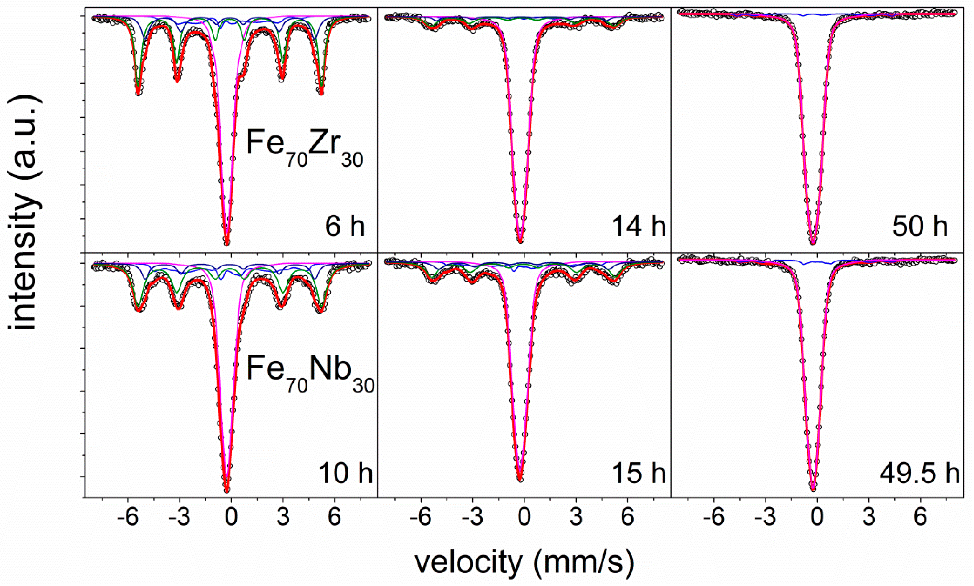
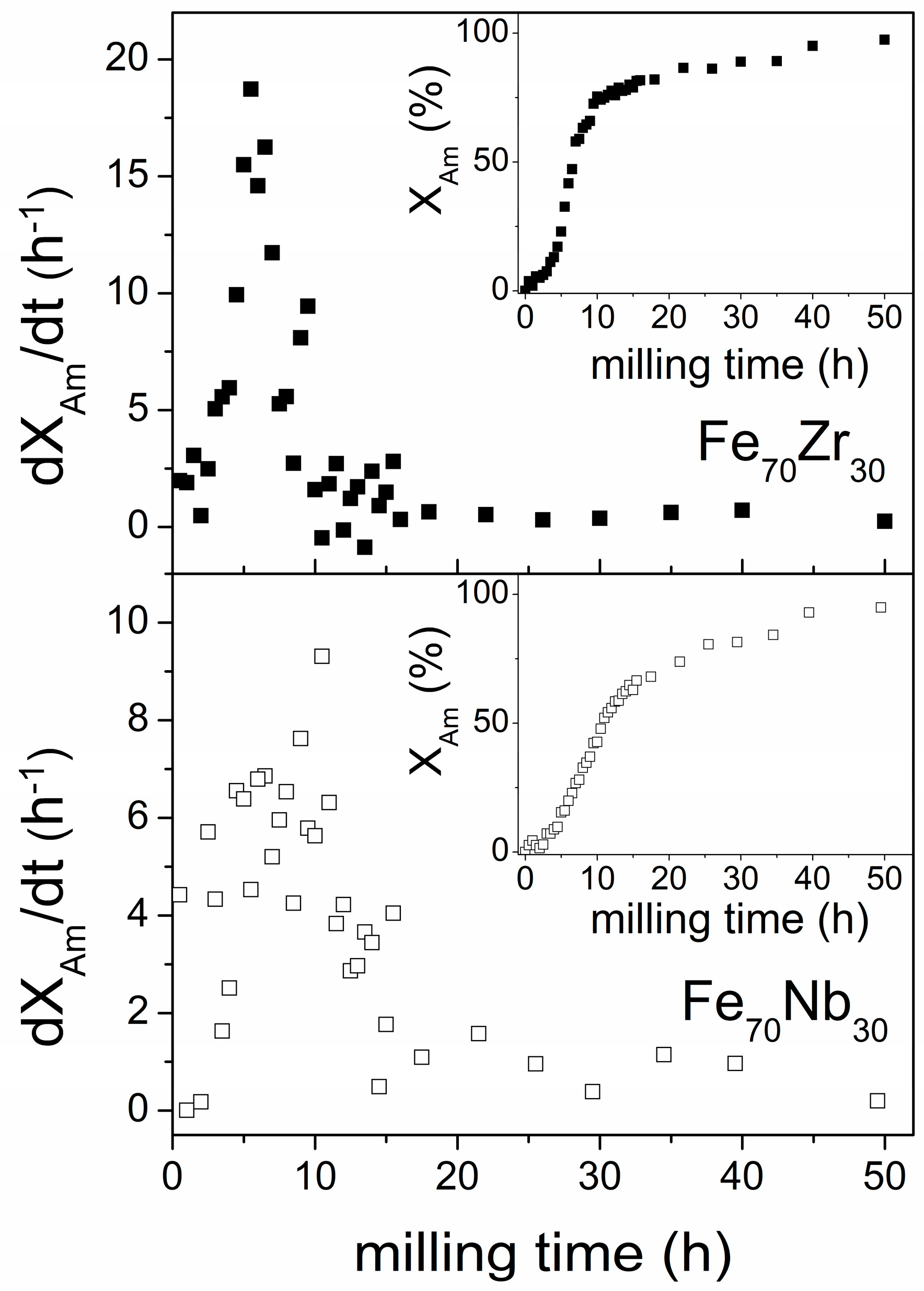
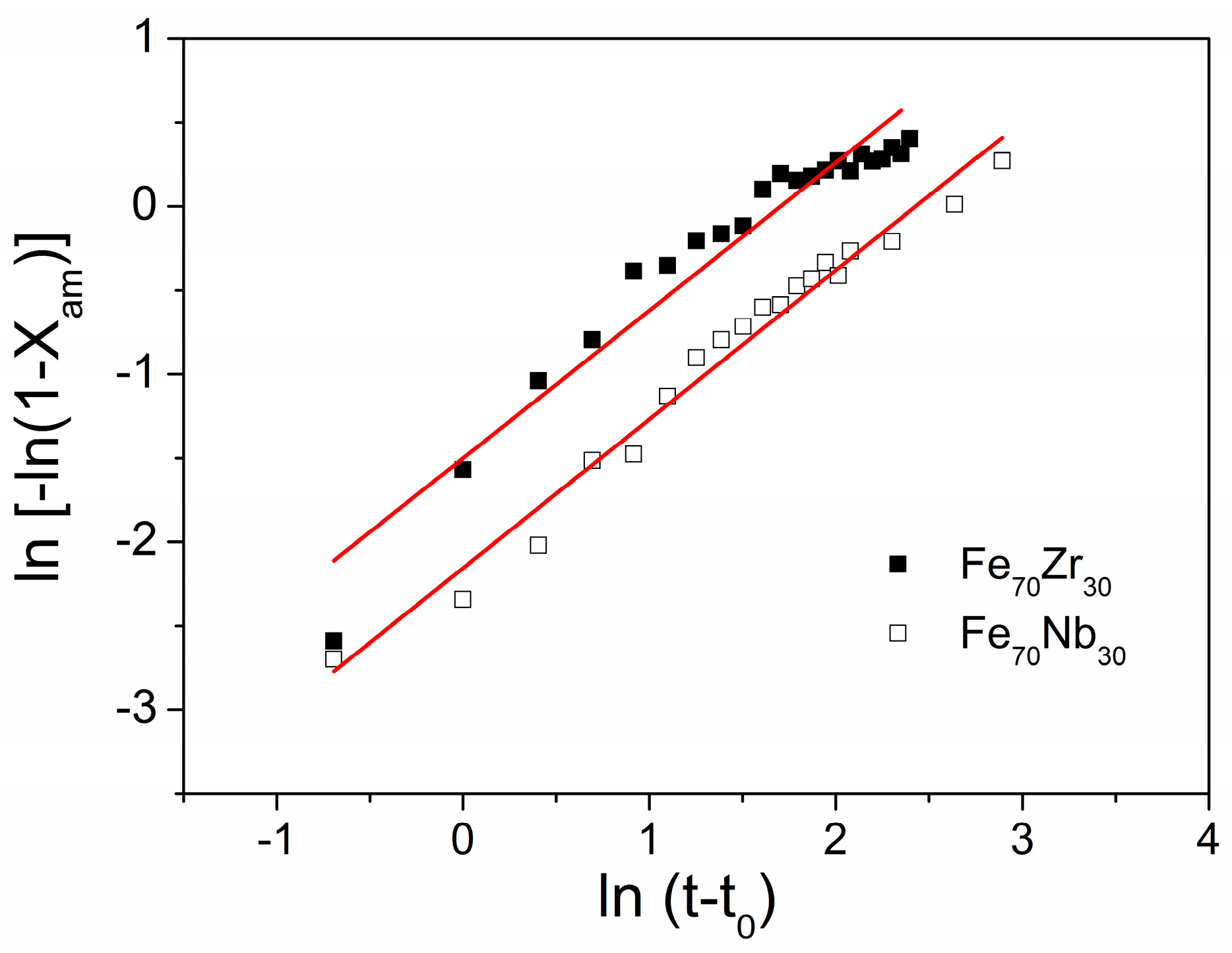
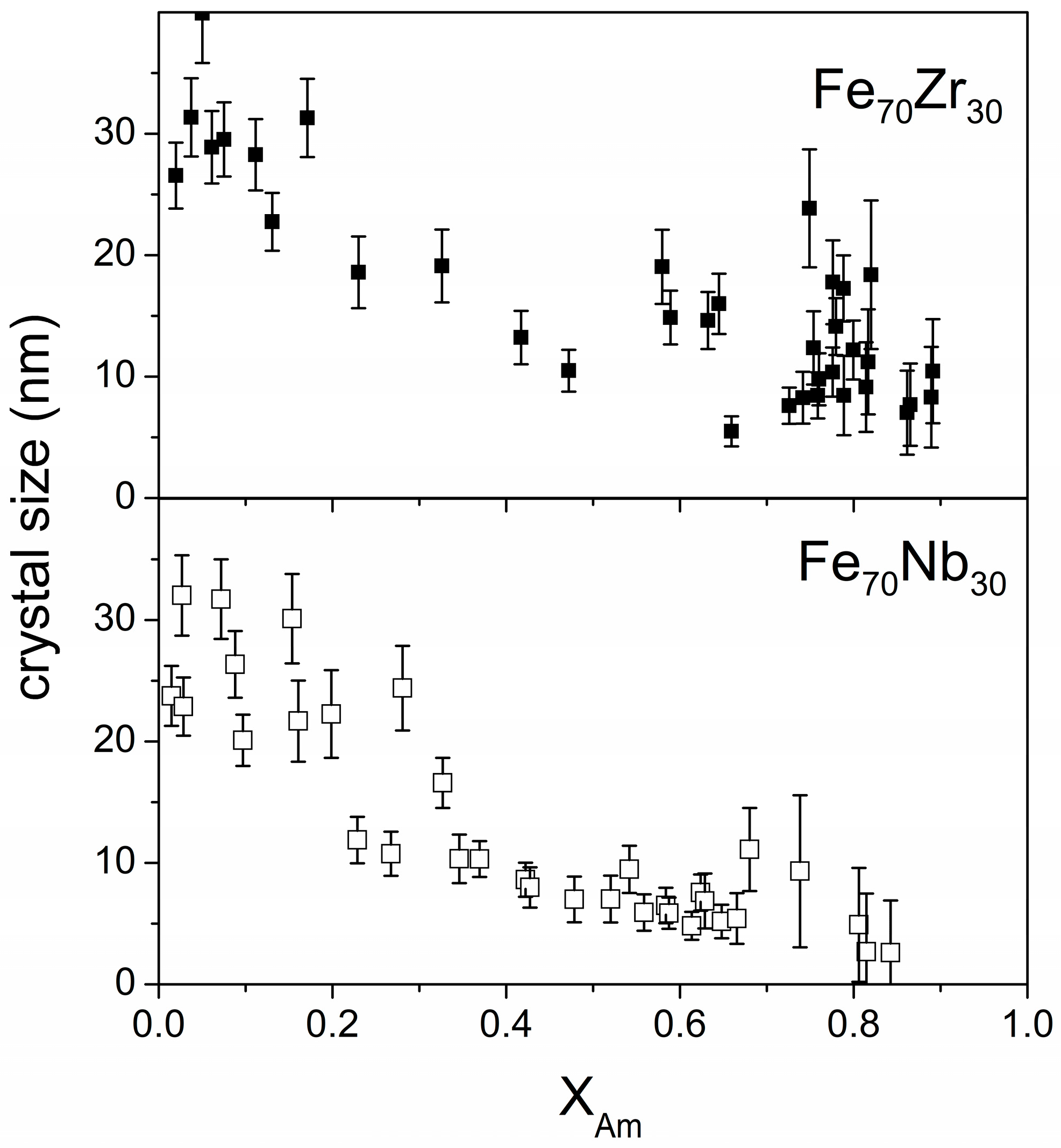
3.4. Experimental Results

Figure 14 shows the Mössbauer spectra along with the fitting components used for the Fe₇₀Zr₃₀ and Fe₇₀Nb₃₀ mechanically alloyed samples at different milling times. Ferromagnetic contributions are ascribed as Fe atoms in the remnant bcc Fe-type crystallites under the following conditions: at 33 T, Fe surrounded by 8 Fe as near neighbors and 6 Fe as next near neighbors; and at 31 T, Fe with a Zr/Nb atom in the first two shells and a hyperfine distribution due to the interface region. The paramagnetic contributions are ascribed to the presence of Fe atoms in the amorphous phase (with a Curie temperature of ~230 K [40]). In fact, the very different Curie temperatures between the crystalline and the amorphous phases containing Fe, being below room temperature for the amorphous and well above room temperature for the bcc Fe, makes Mössbauer spectrometry a very sensitive technique for estimating the ratio between them. This assignment (sextets for Fe atoms in ferromagnetic α-Fe phase and singlets or doublets for Fe atoms in paramagnetic amorphous) is generally found in the literature concerning Mössbauer studies of Fe-Zr and Fe-Nb alloys [41,42,43,44,45] with similar compositions to those studied here. Further details on the microstructures of the studied samples can be found in [23].

Figure 15 shows the X_Am and dX_Am/dt curves against the milling time from data obtained from Mössbauer spectra of the Fe₇₀Zr₃₀ and Fe₇₀Nb₃₀ compositions. There is a maximum dX_Am/dt at t_max~6 and 10 h, respectively. This maximum was predicted by our simulations, while neither the JMAK model with n = 1 nor the D&C model with j = 1 predicted it. Figure 9 shows the t_max ratio between Zr and Nb alloys to be 0.6, implying a ratio between the probabilities P(Zr)/P(Nb)~2.2.

The effective JMAK plots (Figure 16) show that n_eff~0.9. This low value, close to 1, agrees with the values obtained from the simulations.

Table 1. Avrami exponents obtained for mechanical amorphization processes.

Composition	Avrami Exponent	XAm Range (%)	Experimental Technique	Reference
Fe27.9Nb2.2B69.9	1	0–90	Mössbauer	[30]
Cystine	0.46	25–100	XRD	[31]
Fe-6wt. %Mo	0.83 ± 0.05 0.33 ± 0.04	30–60 60–80	XRD	[32]
Cr20Co80	0.81	10–60	XRD	[33]
Ni50Co50	0.34	60–75	XRD	[34]
Ni15Fe5Mo80	1.049	10–70	XRD	[35]
Cu-10wt. %Nb	1.3	0–10	XRD	[36]
Fe70Zr30	0.88 ± 0.05	20–80	Mössbauer	This work
Fe70Nb30	0.89 ± 0.03	30–80	Mössbauer	This work

displays different n_eff values describing mechanical amorphization processes from the literature [30,31,32,33,34,35,36] along with the explored ranges and techniques used to determine X_Am. In general, the direct application of JMAK theory to mechanical amorphization leads to Avrami exponents close to 1, but it is remarkable that they are generally below 1, in agreement with our present experimental results. Deviations from n_eff = 1 could be due to the previously described experimental artifacts. Therefore, from the present results it can be observed that, except for the case where j = 1, the D&C model cannot reproduce the experimentally observed Avrami exponents.

From the experimental intercepts of the JMAK plots of Figure 16 at X_Am~0.2 and 0.1, for Nb and Zr-containing alloys, respectively, we obtained k_eff~0.2 and 0.1 h⁻¹ for the Zr and Nb-containing alloys, respectively. Taking into account the results from Figure 11, these values should be the minimum limits for fP, as k_eff/fP ≤ 1. The milling parameters and media were the same for all the compositions and, therefore, f must have been equivalent. Therefore, the ratio of the probabilities from this analysis, P(Zr)/P(Nb)~2, is in good agreement with that obtained previously from the analysis of t_max values.

Figure 17 shows the experimental results regarding the size evolution of the remaining crystallites of the studied mechanically-alloyed systems as a function of the amorphous fraction. This plot prevents the consideration of those times before the onset of the transformation when there is a strong reduction in the crystal size before amorphization [2,8]. In the studied cases, the crystal sizes reached a saturation value of <R_sat>~10 and 5 nm for Zr and Nb-containing alloys, respectively. However, the size of the nanocrystals just before their activation (required to normalize the values to allow them to be compare with those of Figure 13) could not be well established due to theoverlapping effect of the conventional nanocrystal comminution that occurs during milling. A more reliable parameter should be X_Am^sat, the transformed fraction at which the stable <R_sat> is achieved. For the studied systems, X_Am^sat ≤ 0.4 for both alloys. Taking into account the results from Figure 13, P(G/L₀)⁻¹ < 0.5. This places our studied alloys in the range where n_eff should be close to 1 in Figure 11, in agreement with our JMAK analysis. Overlap with the comminution process or contamination may affect this estimation by shifting X_Am^sat to lower values which should lead to values of n_eff closer to 1.

4. Conclusions

In this work, we discussed two of the models that are generally used to analyze the kinetics of mechanical amorphization, along with a new one based on the probabilistic character of nucleation which assumes a concave growth of the amorphous phase from the edge to the core of the nanocrystals.

It is concluded that, in the case of JMAK model, direct application should be restricted to instantaneous growth cases, as the convex growth considered in the model is not in agreement with the expected behavior during mechanical amorphization. However, the transformation rate is predicted to monotonously decrease (in contrast to the experimental observations), and the size of the remnant crystallites should remain constant during the transformation.

On the other hand, the model imposing a deterministic character for nucleation (determined by number of collisions in which the region is trapped) could not reproduce the effective Avrami exponents. As the transformation of a certain region is assumed to occur suddenly after the activation collision, the size of the remnant crystallites is predicted to be constant during the transformation.

In the frame of the new model developed in this study, simulations based on the probabilistic character of nucleation and the concave growth of the amorphous phase from the boundary to the core of the nanocrystals were in good agreement with the low Avrami exponents and the evolution of the sizes of the remaining crystallites. When instantaneous growth was considered, a JMAK equation with n = 1 was recovered and for very slow growth rates, an effective n_eff = 1.14 was predicted. At intermediate growth rates, a maximum of n_eff = 1.5 was observed. Therefore, the experimentally observed low Avrami exponents were similar to the ones predicted by our model for the complete range.

The simulations reproduced the effective Avrami exponents with n_eff = 1, and predicted the existence of a time at which the transformation rate was maximum, which neither the JMAK, nor D&C model, could predict.

Along with the results found in the literature, we performed experiments on binary alloys to observe the mechanical amorphization process. The experimental results on Fe-based compositions (Fe₇₀Zr₃₀ and Fe₇₀Nb₃₀) were in agreement with the predictions of our simulations and showed slightly lower values of effective Avrami exponents (n_eff~0.9) due to the presence of different artifacts, including the presence of a starting fraction of the amorphous phase at the boundary region between nanocrystals.

The analysis applied to Fe₇₀Zr₃₀ and Fe₇₀Nb₃₀, derived from both t_max and the intercept of the effective JMAK plot, were in good agreement, supporting the model proposed here.

Further studies are welcomed to test the validity of the proposed model through a systematic analysis of the sizes of the remnant crystallites. Moreover, the effect of impurities due to contamination from milling media might lead to artefacts, particularly affecting the data obtained at long milling times. Possible overlapping with other processes induced by milling (i.e., comminution at short milling times, and recrystallization at long milling times) should be also explored in future studies.

References

1. Klement, W.; Willens, R.H.; Duwez, P. Non-crystalline structure in solidified gold-silicon alloys. Nature 1960, 187, 869–870. [Google Scholar] [CrossRef]
2. Suryanarayana, C. Mechanical alloying and milling. Prog. Mater. Sci. 2001, 46, 1–184. [Google Scholar] [CrossRef]
3. Balaz, P.; Achimovicova, M.; Balaz, M.; Billik, P.; Cherkezova-Zheleva, Z.; Criado, J.M.; Delogu, F.; Dutková, E.; Gaffet, E.; Gotor, F.J.; et al. Hallmarks of mechanochemistry: From nanoparticles to technology. Chem. Soc. Rev. 2013, 42, 7571–7637. [Google Scholar] [CrossRef] [PubMed]
4. Yermakov, A.Y.; Yurchikov, Y.Y.; Barinov, V.A. Magnetic-properties of amorphous powders prepared by the mechanical grinding of Y-Co alloys. Fiz. Met. Metallogr. 1981, 52, 1184–1193. [Google Scholar]
5. Koch, C.C.; Cavin, O.B.; McKamey, C.G.; Scarbrough, J.O. Preparation of amorphous Ni60Nb40 by mechanical alloying. Appl. Phys. Lett. 1983, 43, 1017–1019. [Google Scholar] [CrossRef]
6. Schultz, L. Formation of amorphous metals by mechanical alloying. Mater. Sci. Eng. 1988, 97, 15–23. [Google Scholar] [CrossRef]
7. Moreno, L.M.; Blázquez, J.S.; Ipus, J.J.; Borrego, J.M.; Franco, V.; Conde, A. Magnetocaloric effect of Co62Nb6Zr2B30 amorphous alloys obtained by mechanical alloying or rapid quenching. J. Appl. Phys. 2014, 115. [Google Scholar] [CrossRef]
8. Ipus, J.J.; Blázquez, J.S.; Conde, C.F.; Franco, V.; Borrego, J.M.; Lozano-Pérez, S.; Conde, A. Relationship between mechanical amorphization and boron integration during processing of FeNbB alloys. Intermetallics 2014, 49, 98–105. [Google Scholar] [CrossRef] [Green Version]
9. Schwarz, R.B.; Johnson, W.L. Formation of an amorphous alloy by solid-state reaction of the pure polycrystalline metals. Phys. Rev. Lett. 1983, 51, 415. [Google Scholar] [CrossRef]
10. Weeber, A.W.; Bakker, H. Amorphization by ball milling: A review. Phys. B Condens. Matter. 1988, 153, 93–135. [Google Scholar] [CrossRef]
11. Bellon, P.; Averback, R.S. Non-equilibrium roughening of interfaces in crystals under shear: Application to ball milling. Phys. Rev. Lett. 1995, 74, 1819–1822. [Google Scholar] [CrossRef] [PubMed]
12. Hammerberg, J.E.; Holian, B.L.; Röder, J.; Bishop, A.R.; Zhou, S.J. Nonlinear dynamics and the problem of slip at material interfaces. Phys. D Nonlinear Phenom. 1998, 123, 330–340. [Google Scholar] [CrossRef]
13. Lund, A.C.; Schuh, C.A. Atomistic simulation of strain-induced amorphization. Appl. Phys. Lett. 2003, 82. [Google Scholar] [CrossRef]
14. Delogu, F.; Cocco, G. Molecular dynamics investigation on the role of sliding interfaces and friction in the formation of amorphous phases. Phys. Rev. B 2005, 71. [Google Scholar] [CrossRef]
15. Kolmogorov, A.N. On the statistical theory of the crystallization of metals. Bull. Acad. Sci. USSR 1937, 1, 355–359. [Google Scholar]
16. Johnson, W.A.; Mehl, R.F. Reaction kinetics in processes of nucleation and growth. Trans. Am. Inst. Min. Metall. Eng. 1939, 135, 416–442. [Google Scholar]
17. Avrami, M. Granulation, phase change, and microstructure kinetics of phase change. III. J. Chem. Phys. 1941, 9, 177–184. [Google Scholar] [CrossRef]
18. Siegrist, M.E.; Siegfried, M.; Löffler, J.F. High-purity amorphous Zr52.5Cu17.9Ni14.6Al10Ti5 powders via mechanical amorphization of crystalline pre-alloys. Mater. Sci. Eng. A 2006, 418, 236–240. [Google Scholar] [CrossRef]
19. Delogu, F.; Takacs, L. Mechanochemistry of Ti–C powder mixtures. Acta Mater. 2014, 80, 435–444. [Google Scholar] [CrossRef]
20. Burbelko, A.A.; Fras, E.; Kapturkiewicz, W. About Kolmogorov’s statistical theory of phase transformation. Mater. Sci. Eng. A 2005, 413, 429–434. [Google Scholar] [CrossRef]
21. Ipus, J.J.; Blázquez, J.S.; Lozano-Pérez, S.; Conde, A. Microstructural evolution characterization of Fe-Nb-B ternary systems processed by ball milling. Philos. Mag. 2009, 89, 1415–1423. [Google Scholar] [CrossRef]
22. Delogu, F.; Cocco, G. Kinetics of amorphization processes by mechanical alloying: A modeling approach. J. Alloy. Compd. 2007, 436, 233–240. [Google Scholar] [CrossRef]
23. Manchón-Gordón, A.F.; Ipus, J.J.; Blázquez, J.S.; Conde, C.F.; Conde, A. Evolution of Fe environments and phase composition during mechanical amorphization of Fe70Zr30 and Fe70Nb30 alloys. J. Non-Cryst. Solids 2018, 494, 78–85. [Google Scholar] [CrossRef]
24. Delogu, F. A combined experimental and numerical approach to the kinetics of mechanically induced phase transformations. Acta Mater. 2008, 56, 905–912. [Google Scholar] [CrossRef]
25. Blázquez, J.S.; Ipus, J.J.; Moreno-Ramírez, L.M.; Álvarez-Gómez, J.M.; Sánchez-Jiménez, D.; Lozano-Pérez, S.; Franco, V.; Conde, A. Ball milling as a way to produce magnetic and magnetocaloric materials: A review. J. Mater. Sci. 2017, 52, 11834–11850. [Google Scholar] [CrossRef]
26. Blázquez, J.S.; Ipus, J.J.; Conde, A. Time evolution of mechanical amorphization: A kinetic model. Scr. Mater. 2017, 130, 260–263. [Google Scholar] [CrossRef]
27. Blázquez, J.S.; Ipus, J.J.; Franco, V.; Conde, C.F.; Conde, A. Extracting the composition of nanocrystals of mechanically alloyed systems using Mössbauer spectroscopy. J. Alloy. Compd. 2014, 610, 92–99. [Google Scholar] [CrossRef] [Green Version]
28. Burke, J. The Kinetics of Phase Transformations in Metals; Pergamon: Oxford, UK, 1965. [Google Scholar]
29. Chen, B.; Lutker, K.; Raju, S.V.; Yan, J.; Kanitpanyacharoen, W.; Lei, J.; Yang, S.; Wenk, H.R.; Mao, H.K.; Williams, Q. Texture of nanocrystalline nickel: Probing the lower size limit of dislocation activity. Science 2012, 338, 1448–1451. [Google Scholar] [CrossRef] [PubMed]
30. Alleg, S.; Hamouda, A.; Azzaza, S.; Bensalem, R.; Sunol, J.J.; Greneche, J.M. Solid state amorphization transformation in the mechanically alloyed Fe27.9Nb2.2B69.9 powders. Mater. Chem. Phys. 2010, 122, 35–40. [Google Scholar] [CrossRef]
31. Konishi, Y.; Kadota, K.; Tozuka, Y.; Shimosaka, A.; Shirakawa, Y. Amorphization and radical formation of cystine particles by a mechanochemical process analyzed using DEM simulation. Powder Technol. 2016, 301, 220–227. [Google Scholar] [CrossRef]
32. Moumeni, H.; Alleg, S.; Greneche, J.M. Formation of ball-milled Fe-Mo nanostructured powders. J. Alloy. Compd. 2006, 419, 140–144. [Google Scholar] [CrossRef]
33. Louidi, S.; Bentayeb, F.Z.; Sunol, J.J.; Escoda, L. Formation study of the ball-milled Cr20Co80 alloy. J. Alloy. Compd. 2010, 493, 110–115. [Google Scholar] [CrossRef]
34. Loudjani, N.; Bensebaa, N.; Alleg, S.; Djebbari, C.; Greneche, J.M. Microstructure characterization of ball-milled Ni50Co50 alloy by Rietveld method. Phys. Stat. Sol. Appl. Mater. Sci. 2011, 208, 2124–2129. [Google Scholar] [CrossRef]
35. Shen, Y.P.; Hng, H.H.; Oh, J.T. Formation kinetics of Ni-15% Fe-5% Mo during ball milling. Mater. Lett. 2004, 58, 2824–2828. [Google Scholar] [CrossRef]
36. Lei, R.S.; Wang, M.P.; Wang, H.P.; Xu, S.Q. New insights on the formation of supersaturated Cu-Nb solid solution prepared by mechanical alloying. Mater. Character. 2016, 118, 324–331. [Google Scholar] [CrossRef]
37. Abdellaoui, M.; Gaffet, E. The physics of mechanical alloying in a planetary ball mill—Mathematical treatment. Acta Metall. Mater. 1995, 43, 1087–1098. [Google Scholar] [CrossRef]
38. Concas, A.; Lai, N.; Pisu, M.; Cao, G. Modelling of comminution processes in Spex Mixer/Mill. Chem. Eng. Sci. 2006, 61, 3746–3760. [Google Scholar] [CrossRef]
39. Ipus, J.J.; Blázquez, J.S.; Franco, V.; Millán, M.; Conde, A.; Oleszak, D.; Kulik, T. An equivalent time approach for scaling the mechanical alloying processes. Intermetallics 2008, 16, 470–478. [Google Scholar] [CrossRef]
40. Blázquez, J.S.; Franco, V.; Conde, A. Enhancement of the magnetic refrigerant capacity in partially amorphous Fe70Zr30 powders obtained by mechanical alloying. Intermetallics 2012, 26, 52–56. [Google Scholar] [CrossRef]
41. Pizarro, R.; Barandiarán, J.M.; Plazaola, F.; Gutiérrez, J. Synthesis and characterization of amorphous Fe75Zr25 obtained by ball milling. J. Magn. Magn. Mater. 1999, 203, 143–145. [Google Scholar] [CrossRef]
42. Vélez, G.Y.; Alcázar, G.A.P.; Zamora, L.E.; Tabares, J.A. Structural and magnetic study of the Fe2Nb alloy obtained by mechanical alloying and sintering. J. Supercond. Nov. Magn. 2014, 27, 1279–1283. [Google Scholar] [CrossRef]
43. Concas, G.; Congiu, F.; Spano, G.; Bionducci, M. Investigation of the ferromagnetic order in crystalline and amorphous Fe2Zr alloys. J. Magn. Magn. Mater. 2004, 279, 421–428. [Google Scholar] [CrossRef]
44. Povstugar, V.; Butyagin, P.Y.; Dorofeev, G.A.; Elsukov, E.P. Kinetics of the initial stage of mechanical alloying in the Fe(80)Zr(20) system. Colloid J. 2002, 64, 178–185. [Google Scholar] [CrossRef]
45. Pizarro, R.; Garitaonandia, J.S.; Plazaola, F.; Barandiarán, J.M.; Grenèche, J.M. Magnetic and Mössbauer study of multiphase Fe-Zr amorphous powders obtained by high energy ball milling. J. Phys. Condens. Matter 2000, 12, 3101–3112. [Google Scholar] [CrossRef]
Figure 1. Transformed fraction and transformation rate as a function of normalized time for a JMAK system with n = 1.
Metals 08 00450 g001
Figure 2. Effect of indetermination of the induction time (above) and the normalized transformed fraction (below) on the JMAK plot; k = 0.01. Explored range 0.1 < XAm < 0.9.
Metals 08 00450 g002
Figure 3. Effective values of the frequency factor and the Avrami exponent as function of the starting fraction of amorphous phase.
Metals 08 00450 g003
Figure 4. Delogu and Cocco’s (D&C) model. Numerical solutions of Equation (9), XAm(t), and Equation (10), dXAm(t)/dt, for different values of j.
Metals 08 00450 g004
Figure 5. Effective JMAK plots built using the numerical solutions of Equation (9) for different values of j. The units of this parameter are iteration steps, where k’ = 0.1 steps−1.
Metals 08 00450 g005
Figure 6. Effective frequency factors and effective Avrami exponents of numerical solutions of the D&C model as a function of the number of collisions required to activate a region, j, in iteration step units, where k’ = 0.1 steps−1.
Metals 08 00450 g006
Figure 7. The amorphous fraction (XAm) as a function of the iteration steps times the fraction of sample treated per simulation step using f(G/L0) = 0.005 steps−1.
Metals 08 00450 g007
Figure 8. dXAm/dt as a function of the iteration steps times the fraction of sample treated per simulation step using f(G/L0) = 0.005 steps−1.
Metals 08 00450 g008
Figure 9. Time taken for the maximum dXAm/dt from the simulations to occur as a function of the probability of nucleation. The solid lines are the linear fitted data.
Metals 08 00450 g009
Figure 10. Effective JMAK plots using the data obtained from the simulations for different values of nucleation probability and a relative growth rate of fG/L0 = 0.05 step−1. The red lines are the corresponding linear fitted data. The time units are iteration steps.
Metals 08 00450 g010
Figure 11. Effective Avrami exponents and normalized effective frequency factors as a function of P(G/L0)−1, obtained from different sets of simulations, i.e., fixing G/L0 and f and varying P (solid symbols) or fixing P and f and varying G/L0 (hollow symbols and crosses). The results are rescaled to show unique behaviors.
Metals 08 00450 g011
Figure 12. Normalized average radii of the remnant crystallites as a function of the transformed fraction obtained from the simulations for different values of nucleation probability (f(G/L0) = 0.005 steps−1).
Metals 08 00450 g012
Figure 13. Minimum observable relative radii, <R>sat, and transformed fraction at which these values are reached, XAmsat, as a function of P(G/L0)−1.
Metals 08 00450 g013
Figure 14. Mössbauer spectra for Fe70Zr30 and Fe70Nb30 alloys after different milling times.
Metals 08 00450 g014
Figure 15. dXAm/dt obtained from Mössbauer data as a function of milling time for Fe70Zr30 and Fe70Nb30 alloys. The insets show XAm as the paramagnetic phase contribution.
Metals 08 00450 g015
Figure 16. JMAK plots for the studied compositions using data in the ranges indicated in Table 1.
Metals 08 00450 g016
Figure 17. Evolution of experimental sizes of the remaining crystallites as a function of the transformed fraction for the studied alloys.
Metals 08 00450 g017