Mean Stress Effect on the Axial Fatigue Strength of DIN 34CrNiMo6 Quenched and Tempered Steel

Abstract

The present study consists of a theoretical and experimental investigation of the effect of axial mean stresses on the high cycle fatigue behaviour of DIN 34CrNiMo6 high strength steel in quenched and tempered conditions. The axial S-N curves under 4 different stresses ratios were obtained. Experimental results show that increasing the value of the tension mean stresses gradually reduces the axial stress amplitude the material can withstand without failure. Moreover, the compressive mean stresses show a beneficial effect in terms of the axial fatigue strength, resulting in a non-symmetrical Haigh diagram. A historic review of the axial mean stress effect is presented, showing the shape of the Haigh diagrams for ductile metals and presenting the most-known empirical and physical theories. The results for this steel are compared with the physical theories of Findley based on the critical plane; the Froustey’s and Marin’s methods, based on energetic theories; and the Crossland invariants method based on the Gough’s theory of fatigue damage. Taking into account the experimental results, a physical fatigue function based on energetic considerations is proposed. Its application to the fatigue case with mean stresses can be interpreted in terms of a balance of elastic energies of distortion and volume change. Macro-analyses of specimen fracture appearance were conducted in order to obtain the fracture characteristics for different mean stress values.

1. Introduction

1.1. Historical Background

The objective of this study is to determine the mean stress effect on the fatigue behaviour of quenched and tempered DIN 34CrNiMo6 steel with tensile strength σ_uts = 1210 MPa and tensile yield strength σ_yp = 1084 MPa, in order to obtain a theoretical model based on physical principles which could be used to model its behaviour under any combination of mean and variable stresses.

The modelling of the effect of mean stresses is a matter of paramount importance in the fatigue field. In fact, the influence of the mean stress on the fatigue limit was already described by Wöhler in 1870 [1] as one of the main influential factors in the fatigue strength, decreasing the value of the fatigue limit with the increase in mean tension.

The relative importance of axial mean stresses has been especially pointed out in the exhaustive comparative multiaxial methods performed by Papuga in 2011 [2], which concluded that the ability to correctly collect the effect of mean axial stresses is the most determining factor in the prediction capacity of a multiaxial fatigue method. Although practically all of the multiaxial methods take into account the influence of axial mean stresses, the way in which they treat the effect of the same can differ to a great extent.

In order to model the effect of the mean stresses, a multitude of formulations have been proposed, most of which use the engineering tensile stress σ_uts or the monotonic yield stress σ_yp as one of the parameters. In general, these formulas come from empirical approaches to correlate groups of tests on particular materials. In the literature it is widely documented that there is no general empirical law to relate the effect of mean stress on the fatigue limit [3,4,5].

In Figure 1, the mean axial stress σ_m is expressed as a fraction of the ultimate tensile strength σ_uts, and is plotted as an abscissa; the axial stress amplitude σ_a is expressed as a fraction of the fully reversed axial fatigue limit σ₋₁ and is plotted as an ordinate. As can be seen in Figure 1, in which numerous results from the literature are gathered [6,7,8,9,10,11,12,13,14,15,16], the shape of these lines in the Haigh diagram is indicative of the ductility of the material. It should be noted that most of the results lie within the area drawn between the Smith and elliptical lines.

The elliptical relationship, which is concave downward for any mean stress value, is highly accurate to data on extra-ductile steels; it was proposed by Marin in 1956 [17] and is based in energetic considerations. Its application to the uniaxial fatigue case is shown in Equation (1):

$${\mathsf{\sigma }}_{\mathrm{a}}={\mathsf{\sigma }}_{-1}\cdot \sqrt{1-{\left(\frac{{\mathsf{\sigma }}_{\mathrm{m}}}{{\mathsf{\sigma }}_{\mathrm{uts}}}\right)}^2}$$

(1)

The Smith line [3], whose shape is convex downward, was devised as an empirical criterion to adjust the results of brittle materials. It can be expressed through Equation (2):

$${\mathsf{\sigma }}_{\mathrm{a}}={\mathsf{\sigma }}_{-1}\cdot \frac{1-\raisebox{1ex}{${\mathsf{\sigma }}_{\mathrm{m}}$}\!\left/ \!\raisebox{-1ex}{${\mathsf{\sigma }}_{\mathrm{uts}}$}\right.}{1+\raisebox{1ex}{${\mathsf{\sigma }}_{\mathrm{m}}$}\!\left/ \!\raisebox{-1ex}{${\mathsf{\sigma }}_{\mathrm{uts}}$}\right.}$$

(2)

The different shape in the Haigh diagram for ductile and for fragile materials had an early interpretation by Smith in 1942 [3] in terms of the microstructure: the brittle materials own internal stress raisers.

1.2. Empirical Methods

Historically, the first tests of fatigue with mean stresses were performed by Wöhler [1]. Using this data, Gerber [18] proposed in 1884 the following parabolic equation, known as the Gerber line or relation, which was originally expressed through Equation (3):

$${\mathsf{\sigma }}_{\mathrm{a}}={\mathsf{\sigma }}_{-1}\cdot \left[1-{\left(\frac{{\mathsf{\sigma }}_{\mathrm{m}}}{{\mathsf{\sigma }}_{\mathrm{uts}}}\right)}^2\right]$$

(3)

As can be inferred from Equation (3), the sign of the mean stress σ_m has no influence on the alternating stress as it appears in squared form. This equation was fitted with precision to the experimental data available at the time, when the tests with mean compression stresses were not possible. As it was known that the mean compression loads are less damaging than the tensile ones, by proposing a symmetric method with respect to the mean stresses as the parabola (2), the results in compression would be on the safe side. Thus, Gerber’s main objective was to provide an empirical design line adequate for mechanical engineering practice [11].

The work by O’Connor and Morrison in 1956 [11] was the first investigation with machinery able to correctly apply compressive loads, showing a detrimental effect of the compressive mean stresses for some materials. Later investigations confirmed this fact, as shown in Figure 2, where the results on 6 ductile steels and aluminium alloys extracted from the literature [11,12,13,19,20] are presented in a Haigh diagram, showing concave downward shapes. For instance, the effect of the compressive mean stresses appear to be as deleterious as the tension mean stresses for the 25CrMo4 steel [13] (Figure 2), showing a nearly symmetrical diagram.

For partly-brittle materials, the straight line is assumed as the best approximation [21]. Several authors have developed linear theories. In 1922, the Goodman’s theory [22] was modified by Haigh [23]. The modified Goodman criterion can be expressed through Equation (4):

$${\mathsf{\sigma }}_{\mathrm{a}}={\mathsf{\sigma }}_{-1}\cdot \left(1-\frac{{\mathsf{\sigma }}_{\mathrm{m}}}{{\mathsf{\sigma }}_{\mathrm{uts}}}\right)$$

(4)

Another straight line approach is the contribution by Morrow [24], who proposed a modification of Equation (4) by replacing the ultimate tensile strength σ_uts with the fracture strength σ_fB corrected by Bridgman [25], resulting in Equation (5):

$${\mathsf{\sigma }}_{\mathrm{a}}={\mathsf{\sigma }}_{-1}\cdot \left(1-\frac{{\mathsf{\sigma }}_{\mathrm{m}}}{{\mathsf{\sigma }}_{\mathrm{fB}}}\right)$$

(5)

Morrow’s equation offers improved agreement with experimental results of steels when compared to Goodman’s line according to some sources in the literature [26,27]. However, true fracture strengths with the Bridgman correction are difficult to obtain and therefore usually unavailable, so that they have to be estimated. A common estimation found in the literature is the one proposed by Dowling et al. [26], which is usually considered to be valid up to 1700 MPa, and represented in Equation (6):

$${\mathsf{\sigma }}_{\mathrm{fB}}={\mathsf{\sigma }}_{\mathrm{uts}}+345\mathrm{MPa}$$

(6)

Another commonly used empirical correlation corresponds to Dietmann [28], who in the 70s of the 20th century proposed the relationship represented by Equation (7):

$${\mathsf{\sigma }}_{\mathrm{a}}={\mathsf{\sigma }}_{-1}\cdot \sqrt{1-\frac{{\mathsf{\sigma }}_{\mathrm{m}}}{{\mathsf{\sigma }}_{\mathrm{uts}}}}$$

(7)

This relationship shows a high statistical correlation with experimental data for tensile mean stresses due to the fact that is located between the lines of Goodman and Gerber for most of the range of R in axial mean stresses, where most of the experimental points are located according to some collections of data from the literature [29]. For compressive mean loads, the fatigue strength increases with the value of the compressive mean stress, showing a beneficial effect.

1.3. Methods Based on Physical Principles

In contrast to the Gerber, Goodman, Morrow and Dietmann empirical lines, some theories were developed on the basis of physical principles to explain the fatigue damage, amongst them the following:

• Gough hypothesis [7]: This theory states that effect of the mean stresses is due only to the damage produced by the maximum stress reached during the cycle, with no regard for the mean stress itself. This assumption led to the Crossland method [30], which uses the maximum hydrostatic stress during the cycle as the damage parameter.
• Distortion energy theory [17]: In a theoretical material of von Mises, the effect of the normal stress to the critical plane is quadratic, without any influence of the hydrostatic stress. Moreover, equating the energies produced in N cycles in the case of completely reversed alternating stresses and the case of superimposed static stresses to a variable stress, an elliptic relationship between the mean and alternating stresses is obtained. This theory can be expressed analytically through the Marin multiaxial fatigue method.
• Total strain energy theory [31]: The effect of the mean stresses is related to the total elastic deformation energy stored. This hypothesis leads to the Froustey method, which leads to an elliptic relationship between the mean and alternating stresses, as in the Marin method.
• Findley critical plane [32]: The normal stress to high shear stress amplitudes planes allow the propagation of a micro-crack initiated by shear stresses. As Findley remarks [33], this effect is approximately linear in some materials, being clearly non-linear in others. For simplicity purposes, a linear normal maximum stress to the critical plane was selected by Findley as one of the damage parameters for the formulation of the Findley critical plane method.

The Crossland method [30] was presented in 1956 after a series of tests on En25T NiCrMo quenched and tempered steel, including mean stress effect fatigue loadings [11]. Crossland concluded that a linear function of the square root of the second invariant of the stress deviator and the maximum hydrostatic stress had a good agreement for the majority of the tests on En25T steel. This method was devised according to the Gough theory [7], which states that the fatigue damage provoked by mean stresses is not due to the mean stress itself, but to the maximum stress reached within the cycle. The Crossland method is usually defined through the Equation (8):

$$\sqrt{J_{2,\mathrm{a}}}+{\mathsf{\alpha }}_{\mathrm{C}}\cdot {\mathsf{\sigma }}_{\mathrm{H},\max }\le {\mathsf{\lambda }}_{\mathrm{C}}$$

(8)

where α_c and λ_c are material parameters which can be adjusted with two tests, usually the fully reversed axial fatigue strength σ₋₁, which takes a value of σ₋₁ = 615 MPa for the 34CrNiMo6 steel; and the fully reversed torsional fatigue strength τ₋₁, which was determined through a fifteen specimens staircase, obtaining a value of τ₋₁ = 433 MPa. The calculation of the Crossland parameters could therefore determined with the Equations (9a) and (9b).

$${\mathsf{\alpha }}_{\mathrm{c}}=3\cdot {\mathsf{\tau }}_{-1}/{\mathsf{\sigma }}_{-1}-\sqrt{3}$$

(9a)

$${\mathsf{\lambda }}_{\mathrm{c}}={\mathsf{\tau }}_{-1}$$

(9b)

The application of the Crossland method to the axial fatigue case with mean stresses results in the Equation (10):

$${\mathsf{\sigma }}_{\mathrm{a}}={\mathsf{\sigma }}_{-1}-\left(1-\frac{{\mathsf{\sigma }}_{-1}}{\sqrt{3}\cdot {\mathsf{\tau }}_{-1}}\right)\cdot {\mathsf{\sigma }}_{\mathrm{m}}$$

(10)

Therefore, a linear influence of the mean stress in the axial fatigue case is predicted by the Crossland method. The tensile mean stresses create a detrimental effect in the fatigue strength, and the compressive mean stresses increase the stress amplitude that the material can withstand without failure.

The Marin method [17] is based on the distortion energy theory, and can be expressed through Equation (11):

$${\left(\frac{\sqrt{3}\cdot \sqrt{J_{2,\mathrm{a}}}}{{\mathsf{\sigma }}_{-1}}\right)}^2+{\left(\frac{\sqrt{3}\cdot \sqrt{J_{2,\mathrm{m}}}}{{\mathsf{\sigma }}_{\mathrm{uts}}}\right)}^2\le 1$$

(11)

where $\sqrt{J_{2,\mathrm{a}}}$ and $\sqrt{J_{2,\mathrm{m}}}$ are amplitude and mean value of the square root of the second invariant of the stress deviator, and σ₋₁ the fully reversed axial fatigue strength. Its application to the axial mean stress loading case results in the elliptical relationship given in Equation (12):

$${\mathsf{\sigma }}_{\mathrm{a}}\le {\mathsf{\sigma }}_{-1}\cdot \sqrt{1-{\left(\frac{{\mathsf{\sigma }}_{\mathrm{m}}}{{\mathsf{\sigma }}_{\mathrm{uts}}}\right)}^2}$$

(12)

As can be inferred from Equation (13), Marin’s method is equally sensitive to the tension and compression mean stresses. The Marin’s elliptical relationship shows an excellent agreement with extra-ductile materials, which exhibit a symmetrical shape in the Haigh diagram, such as the 25CrMo4 steel represented in Figure 2.

The Froustey [31] method is based in the total elastic strain energy. Its application to the axial fatigue case with mean stresses lead to the same equation of the Marin method, Equation (12).

The Findley method [32] is a critical plane approach based on the plane that maximises the damage function given by:

$$f(\mathsf{\varphi },\mathsf{\theta })={{\mathsf{\tau }}_{\mathrm{a}}}^{*}(\mathsf{\varphi },\mathsf{\theta })+{\mathsf{\alpha }}_{\mathrm{F}}\cdot {N_{\max }}^{*}(\mathsf{\varphi },\mathsf{\theta })$$

(13)

Once the pair of angles (ϕ*, θ*) for which this function is maximum is obtained, the fatigue indicator parameter given by Equation (13) is computed, where α_F and λ_F are material parameters which can be identified from endurance fatigue limits; usually the fully reversed axial and torsional fatigue limits (σ₋₁ and τ₋₁).

$${{\mathsf{\tau }}_{\mathrm{a}}}^{*}({\mathsf{\varphi }}^{*},{\mathsf{\theta }}^{*})+{\mathsf{\alpha }}_{\mathrm{F}}\cdot {N_{\max }}^{*}({\mathsf{\varphi }}^{*},{\mathsf{\theta }}^{*})\le {\mathsf{\lambda }}_{\mathrm{F}}$$

(14)

Findley’s method can be applied analytically to the axial fatigue loading with mean stresses through Equation (15):

$${\mathsf{\sigma }}_{\mathrm{a}}=2\cdot \sqrt{{\mathsf{\lambda }}_{\mathrm{F}}{}^2\cdot {\mathsf{\alpha }}_{\mathrm{F}}{}^2+{\mathsf{\lambda }}_{\mathrm{F}}{}^2-{\mathsf{\alpha }}_{\mathrm{F}}\cdot {\mathsf{\lambda }}_{\mathrm{F}}\cdot {\mathsf{\sigma }}_{\mathrm{m}}}-2\cdot {\mathsf{\alpha }}_{\mathrm{F}}\cdot {\mathsf{\lambda }}_{\mathrm{F}}$$

(15)

The constants α_F and λ_F depend on the value of the fatigue ratio κ = σ₋₁/τ₋₁. By simple inspection of Equation (15), it can be inferred that if κ takes a value of 2.0, which corresponds to the Tresca criterion, α_F becomes 0.0, so that the mean axial stresses produce no effect on the axial fatigue strength. For materials following the Rankine maximum principal stress criterion, that is: κ ≈ 1, the predicted influence of the mean axial stress is very high. This theory explains the fact that the influence of mean axial stress is small for ductile metals but strong for brittle cast irons. The fatigue ratio κ = σ₋₁/τ₋₁ is equal to 1.42 for the 34CrNiMo6 quenched and tempered steel, therefore takes an intermediate value between the Tresca and Rankine theories.

Despite all the work performed over the years, the effect of the mean stresses remains a problem of great interest in engineering practice, especially because of the introduction and development of mechanical and thermal treatments to introduce residual compression stresses which improve the fatigue strength of mechanical components [34]. Therefore, it is of paramount importance to determine in a very precise way the effect of mean compression loads, in order to correctly evaluate the effectiveness of mechanical and thermal treatments based on the introduction of residual stresses.

The aim of this paper is to obtain the mean stress effect on the fatigue behaviour of DIN 34CrNiMo6 steel, a high strength steel commonly used in the engineering practice. Fatigue tests with different stress ratios have been performed, and comparisons with empirical and physical methods have been analysed. The fatigue data obtained has been used in order to obtain a non-empirical method based on physical principles which can also be used as an analytical model to accurately calculate the mean stress effect on other structural steels, including normalized and quenched and tempered steels. Moreover, it can be applied to multiaxial fatigue stresses, such as taking place in thermal and mechanical treatments, in which residual stresses are inherently multiaxial.

2. Testing Procedure

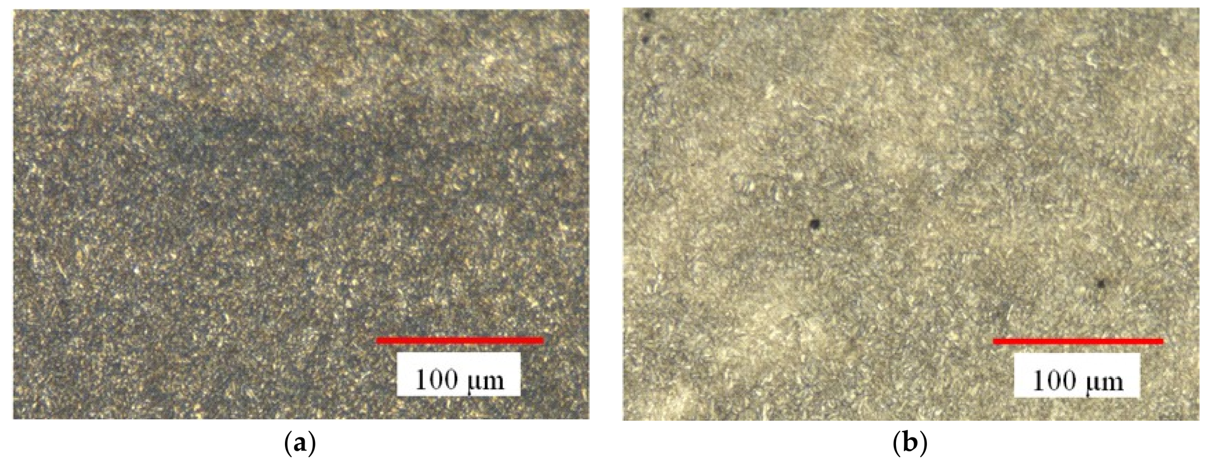
2.1. Material

The material used in the present fatigue campaign is a high strength 34CrNiMo6 steel provided by Thyssen-Krupp in 30 mm diameter forged bars. This steel is commonly used in the engineering practice in axles, shafts, rods, valves, pinions and other engineering parts with a high level of exigency from the point of view of safety and reliability, and its microstructure is well documented in the literature [35,36].

The heat treatment consisted in a normalization at 900 °C, followed by a quenching in oil and a tempering at 570 °C. The resulting microstructure is the well-known ductile tempered martensite which appears as a result of high temperature tempering processes. The main process responsible for the strengthening in this steel is the precipitation of a fine dispersion of alloy carbides during tempering. The certified chemical composition was furnished with the material and is presented in

Table 1. Chemical composition of 34CrNiMo6 high strength steel (at. %).

Element	C	Cr	Ni	Mo	Mn	Si	P	S	Fe
Weight (%)	0.345	1.565	1.565	0.237	0.710	0.275	0.0075	0.003	Balance

. The monotonic mechanical properties of this steel are given in

Table 2. Monotonic mechanical properties of 34CrNiMo6 high strength steel.

Monotonic Properties	Symbol	Value
Yield strength	σyp	1084 MPa
Ultimate tensile strength	σuts	1210 MPa
Reduction of area	Z	60.2%
Elongation at fracture	A	12.2%

, showing a ductile behaviour.

This steel shows a homogenous microstructure based of fine tempered martensite, with a banded orientation of the inclusions in the longitudinal section which cannot be observed in the transversal section (Figure 3a,b). As was observed in other previous investigations regarding this steel, porosity and many inclusions with different sizes were found [36], being round-shaped and small, with maximum defect size equal to $\sqrt{\mathrm{area}}$ ≈ 5 µm.

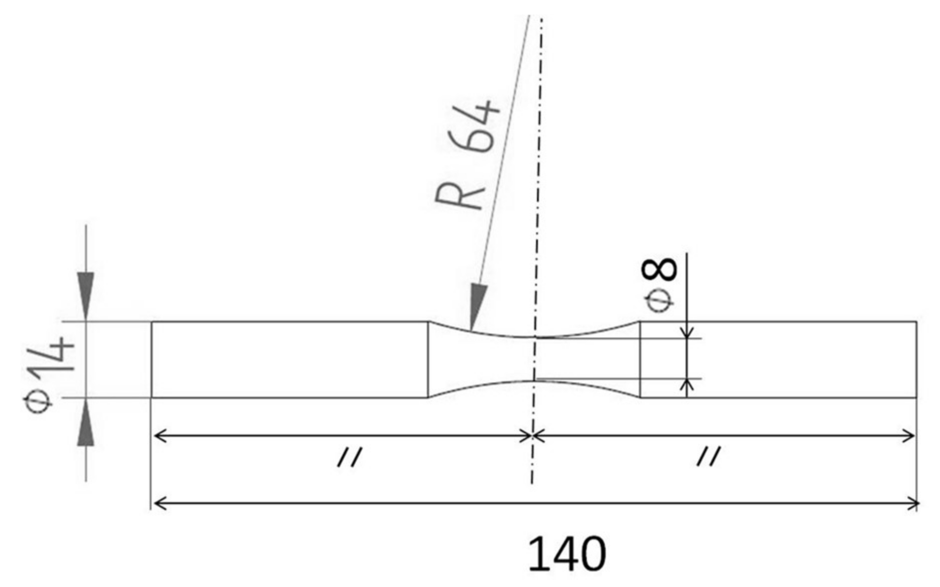
2.2. Specimens and Testing Machine

Fatigue tests were performed on standard hourglass specimens whose dimensions are given in Figure 4. As was pointed out by other authors [37], hourglass geometry promotes the concentration of failures in a very limited area of the specimen, so that the scatter is reduced.

The specimens were designed and manufactured following the recommendations of ASTM E-466 [38]. A final average roughness Ra = 0.03 µm was measured.

Fatigue tests were performed in the laboratories of the Department of Mechanical Engineering of the UPV/EHU (Spain), on a servo-hydraulic axial fatigue machine Instron 8805 MTB (Instron, High Wycombre, UK), with a maximum available axial force of 100 kN. The tests were performed at a frequency of 20 Hz. The run-out was fixed at 2 × 10⁶ cycles. The failure criterion was defined as a 10% loss in rigidity of the specimen.

3. Results and Experimental Correlation with Empirical and Physical Models

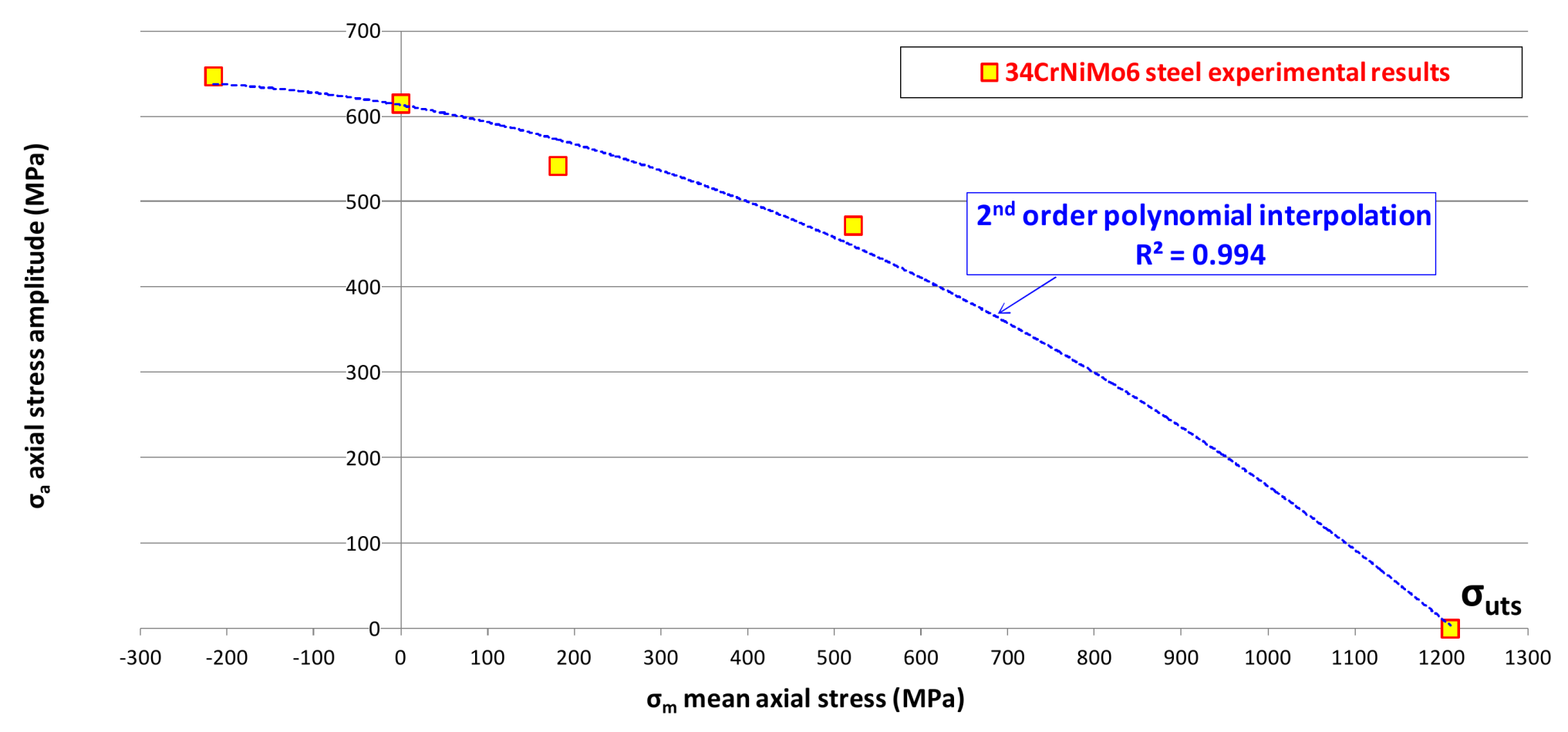
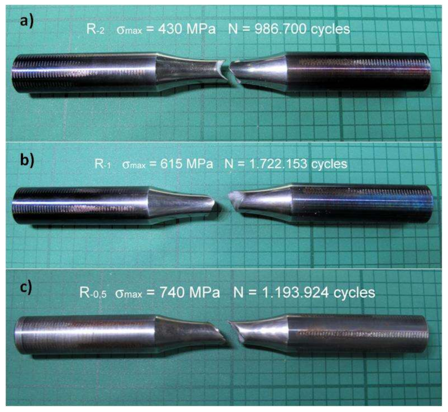
3.1. Fatigue Test Results

An axial fatigue campaign with four different stress ratios R = σ_min/σ_max has been performed, namely R = −2, −1, −0.5 and 0.05, with a total number of 75 specimens considering all the tests. Tests were stopped at a maximum fatigue life of 2 × 10⁶ cycles, taking into account the recommendations for the number of cycles of the fatigue limit for this type of steel [39]. The full S-N curves (P = 50%) were adjusted with the well-known Basquin formulation in the form N = α∙σ^β (α and β values in

Table 3. Obtained fatigue strengths at 2 × 10⁶ cycles for the different stress ratios together with the α and β Basquin parameters of the inclined part of the S-N curves.

σm (MPa)	σa (MPa)	R (Stress Ratio)	α	β
−216	647	−2	1.14 × 1048	−15.000
0	615	−1	4.61 × 1042	−13.220
181	542	−0.5	1.79 × 1031	−9.338
522	472	0.05	6.37 × 1077	−26.889

) commonly used in modern fatigue investigations with quenched and tempered steels as in [40]. In Figure 5 the S-N curves for the different stress ratios are presented, showing a measurable effect of the mean stresses for all the range of fatigue lives: 2 × 10⁴ < N < 2 × 10⁶ cycles. The ASTM E 739 standard has been used to obtain the Basquin parameters. The standard deviation of the fatigue curves is within the range 10–15 MPa for all the stress ratios. Thus, the staircase method according to ISO 12107:2012 with a step of 10 MPa has been adopted for obtaining the fatigue limits.

As it can be observed in Figure 5, the S-N curve for R = 0.05 has a small slope, which is due to the fact that the fatigue limit has a stress amplitude of 472 MPa and an mean stress of 522 MPa. Therefore, the maximum stress is equal to 990 MPa, while σ_yp is 1084 MPa. Thus, there is only a margin of about 90 MPa for the inclined part of the S-N curve.

The results for 2 × 10⁶ cycles are plotted in a Haigh diagram, see Figure 6. A second order polynomial line was used to fit the experimental results, showing a good agreement with them. The results show that the effect of the mean axial stress takes a great role in the fatigue strength. As was shown in Figure 2 for other ductile materials, the results of the 34CrNiMo6 show a concave downward shape function in the Haigh diagram.

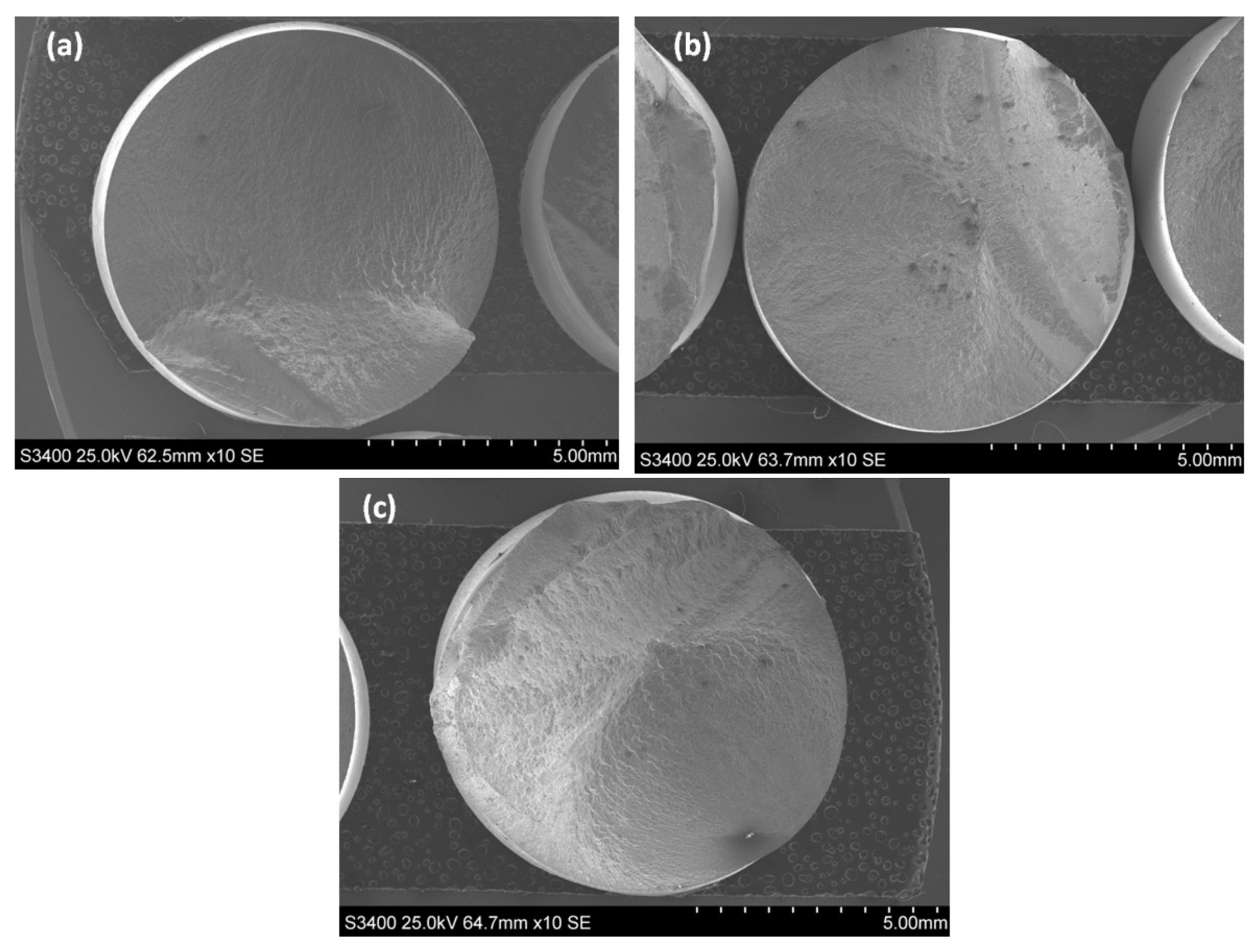
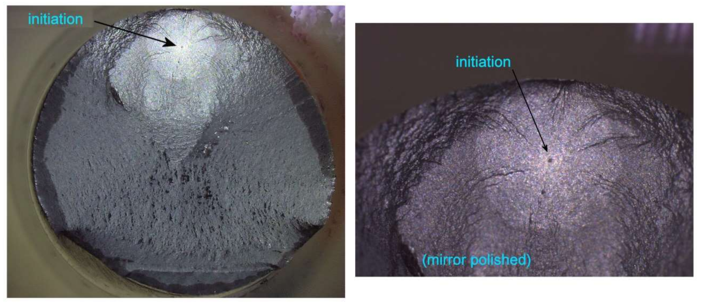
3.2. Fractographic Analysis of the Specimens

Fractographic analysis is not essential for the quantitative purposes of this work, but it enables us to observe the planes of failure and the nature of the fatigue failure. Several previous works have dealt with this particular steel, such as the works of Branco et al. [35,36].

As usually observed in the high cycle fatigue (HCF) region, crack initiation occurred at the very late stage of the fatigue life: a macroscopic crack was not observed until very few cycles before the final fracture. For number of cycles exceeding one million, initiation was produced in general at the surface for the stress ratios R = −2, R = −1, R = −0.5, and R = 0.05 (Figure 7).

However, Figure 8 shows a deep subsurface initiation in an inclusion, which failed about 10⁶ cycles in a R = 0.05 axial test. This failure mode is prone to appear with an increase in the stress ratio in the axial loading, as reported by Gaur et al. [41]. Moreover, a crack initiation beneath the surface is unlikely in rotating-bending tests due to the gradient of the stress field, characteristic of the bending load. Other authors have reported dissimilar behaviours between axial and rotating bending loading [42], remarking that the high cycle failure for rotating bending loading takes place in the surface, and that the internal defects can only create damage for very high cycle fatigue loadings.

The propagation took place in planes approximately corresponding to the maximum shear stress amplitude plane, corresponding to an inclination of 45° to the axis of the specimen (Figure 9).

3.3. Correlation of the Experimental Results with Empirical and Physical Models

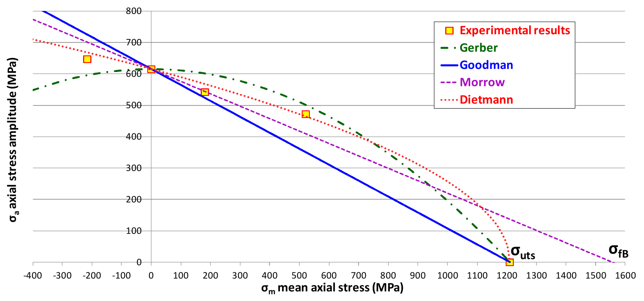
3.3.1. Empirical Models

In Figure 10 the experimental results are shown together with the empirical lines of Gerber, Goodman, Morrow and Dietmann in a Haigh diagram. The fracture strength σ_fB corrected by Bridgman, which is necessary for the Morrow method, was estimated with the Dowling correlation shown in Equation (6). In

Table 4. Relative errors (%) of the different theories: Gerber [18], Goodman [23], Morrow [24] and Dietmann [28] for N = 2 × 10⁶ cycles. Positive values mean conservative results predicted by the theory, negative values non-conservative results.

R (σmin/σmax)	σm (MPa)	Gerber	Goodman	Morrow	Dietmann
−2	−216	8.0	−12.0	−8.3	−3.2
−0.5	181	−10.9	3.5	−0.3	−4.6
0.05	522	−6.1	−25.9	13.4	1.7

, the relative errors (%) of the different theories are presented for N = 2 × 10⁶ cycles. As can be observed, the Dietmann line offers the best agreement with the experimental results. However, the other empirical methods are unable to correctly represent the fatigue behaviour. The Gerber line is not conservative for the tension mean loads. The Goodman line, usually considered as conservative for ductile metals [3,4], shows non-conservative behaviour for the test with compression mean loads. The Morrow line fits the results better than Goodman and Gerber but it is non-conservative in the compression side due to its linear nature.

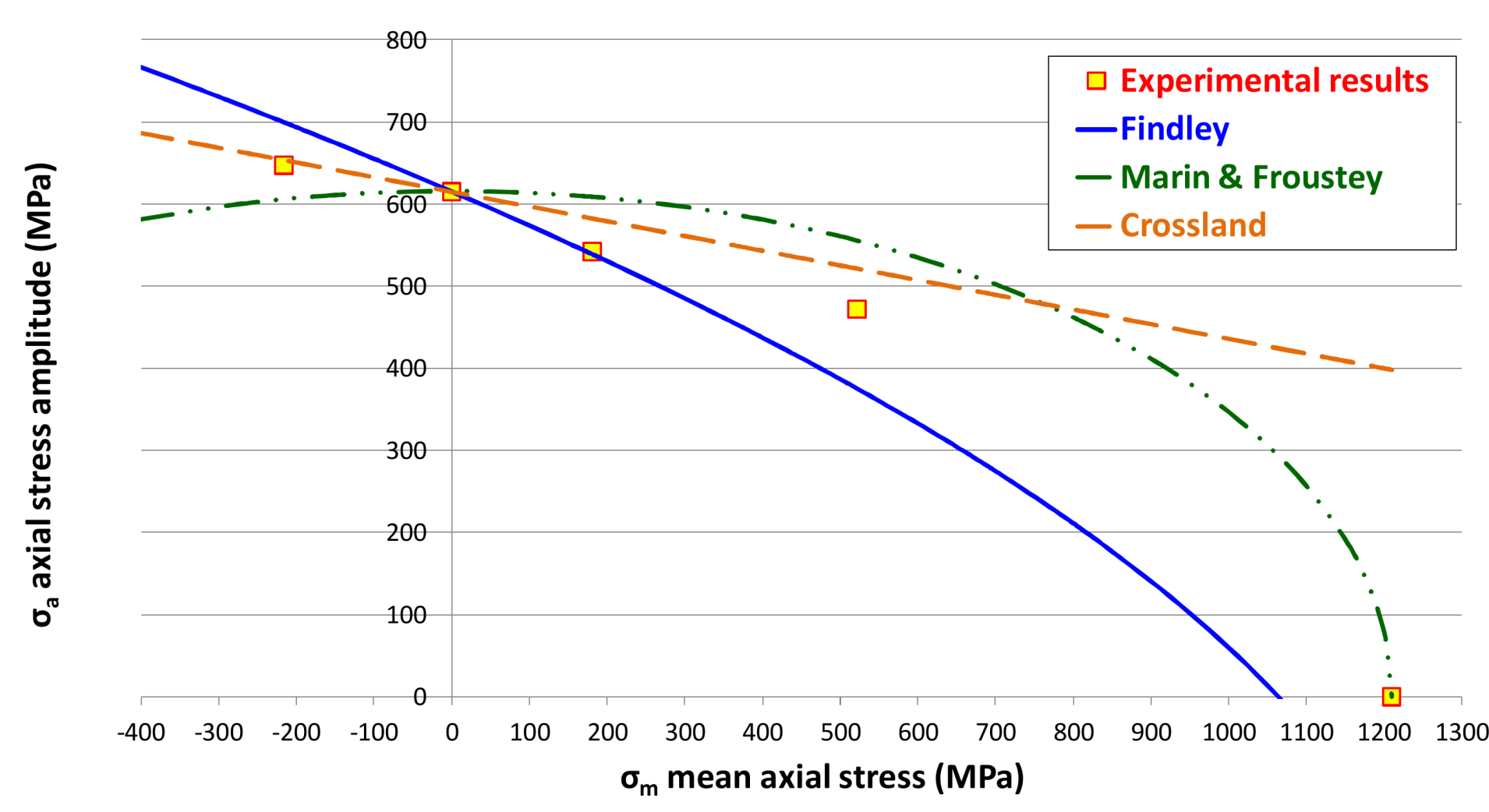
3.3.2. Physical-Based Models

In this section the correlation of the experimental results with different physical principles based theoretical models is analysed. Amongst these fatigue methods, the Crossland [30] method, based on stress invariants, the Findley [32] critical plane method, and the energetic approach based methods of Marin [17] and Froustey [31] will be considered. These methods take into account the effect of mean stresses, and can be easily expressed through analytic formulations for the axial case.

In Figure 11 the four different theoretical predictions by Findley, Marin, Froustey and Crossland are represented in a Haigh diagram together with the experimental results. As observed, none of the methods is able to successfully represent the fatigue behaviour with superimposed static stresses.

In

Table 5. Relative errors (%) of the different theories: Crossland [30], Marin [17], Froustey [31] and Findley [32] for N = 2 × 10⁶ cycles. Positive values mean conservative results predicted by the theory, negative values non-conservative results.

R (σmin/σmax)	σm (MPa)	Crossland	Marin, Froustey	Findley
−2	−216	−1.0	6.5	−8.1
−0.5	181	−7.5	−12.2	0.6
0.05	522	−10.5	−17.6	20.5

, the relative errors (%) of the different theories are presented for N = 2 × 10⁶ cycles. Marin’s and Froustey’s methods are non-conservative with mean tension loads, whereas they show conservative behaviour in the mean compression loads region. It should be noted that the physical methods predicted errors exceed the range (−10%, 10%). The Crossland’s method, which is the most accurate amongst the physical methods, shows non-conservative behaviour for all the analysed cases. The Findley critical plane method is non-conservative for compression mean loads, and highly conservative for the R = 0.05 case.

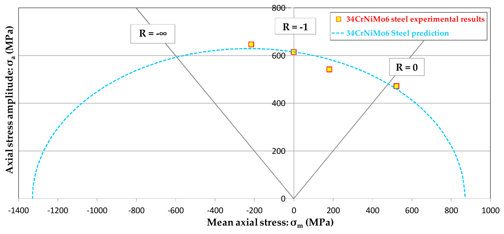
4. Development of an Energetic Fatigue Criterion for a DIN 34CrNiMo6 Quenched and Tempered Steel

As has been commented previously, for engineering applications such as the ones based on treatments which induce compressive residual stresses, it is of paramount importance to have a method that accurately predicts the mean stress effect. Moreover, those residual stresses are generally multiaxial, and the uniaxial empirical methods need some transformations to be adapted to the general multiaxial case.

The formulation of Marin’s method (Equation (11)) is the simplest way to model the axial fatigue problem with mean loads with an energetic approach. However, its application to the axial fatigue loading with mean axial stresses gives a symmetrical Haigh diagram σ_m-σ_a, giving a conservative prediction for the compressive mean stresses. Equation (16) can be interpreted as a balance of distortion energy. The elastic energy of distortion W_D is proportional to the second invariant of the stress deviator tensor J₂. Therefore, Equation (16) equalizes the distortion energy of amplitude to the static distortion energy, where “a” and “b” are constants of the material:

$${\left(\frac{\sqrt{J_{2,\mathrm{a}}}}{\mathrm{a}}\right)}^2+{\left(\frac{\sqrt{J_{2,\mathrm{m}}}}{\mathrm{b}}\right)}^2=1$$

(16)

The constants “a” and “b” of Equation (16) represent respectively the alternating and static von Mises stress at which the material fails [17]. The elliptical shape represented by Equation (16) is suitable for extra ductile materials in which the compressive mean stresses are as damaging as the tensile mean stresses, as it is shown in Figure 1. However, it is widely accepted in the literature that the Haigh diagrams are generally non-symmetrical, even for ductile materials, as it is shown in Figure 2. Therefore the main criticism related to the Marin’s method is the non influence of the sign and magnitude of the hydrostatic stresses [43,44].

In order to take into account the influence of the hydrostatic stresses and the non-symmetrical shape of the Haigh diagram, a new formulation is proposed by modifying the Marin equation, by including the mean value of the first invariant of the stress tensor I_1,m, resulting in Equation (17):

$${\left(\frac{\sqrt{J_{2,\mathrm{a}}}}{\mathrm{a}}\right)}^2+{\left(\frac{\sqrt{J_{2,\mathrm{m}}}}{\mathrm{b}}\right)}^2+{\left(\frac{I_{1,\mathrm{m}}+\Lambda }{\mathrm{c}}\right)}^2=1$$

(17)

The third term of the Equation (17) represents the stored mean hydrostatic energy, which is proportional to the squared value of the first invariant of the stress tensor I_1,m, and related to the energy required to change the volume. The parameter Λ, which can take a value equal or higher than zero, allows a symmetry breaking of the Haigh diagram, as was predicted by the mesoscopic theory of Papadopoulos [43], which states that the hydrostatic stresses create a non-symmetrical Haigh diagram. Moreover, the constant Λ is linked with the hydrostatic stresses in the volume defects, which, according to the Gurson theory, would increase the static strength in compression compared to that in tension [45], as Equation (17) predicts when the parameter Λ takes a value higher than 0.

The parameter “c” of Equation (17) is a material constant which represents the static hydrostatic load at which the material fails, and according to Bridgman’s extensive work [25], this constant should be higher than the constant “b”, as ductile materials are more susceptible to fail from shear stresses than from hydrostatic stresses.

The determination of the parameters can be done with 4 different tests in order to determine the 4 constants “a”, “b”, “c” and “Λ”. Following the procedure of Zenner et al. [46], the four different selected test are the fully reversed axial and torsional fatigue limits σ₋₁ and τ₋₁, the repeated axial and torsional fatigue limits σ₀ and τ₀. The algebraic determination of the values of the constants “a”, “b”, “c” and “Λ” is presented in Appendix A, and their values shown in Equations (18a)–(18d):

$$\mathrm{a}={\mathsf{\tau }}_{-1}$$

(18a)

$$\mathrm{b}=\frac{{\mathsf{\tau }}_0}{2\sqrt{1-\left(\frac{{\mathsf{\tau }}_0}{2\cdot {\mathsf{\tau }}_{-1}}\right)}}$$

(18b)

$$\mathrm{c}=\frac{{\mathsf{\sigma }}_0}{2\cdot \left(\sqrt{1-{\left(\frac{{\mathsf{\sigma }}_0}{2\sqrt{3}}\right)}^2\cdot \left(\frac{1}{{\mathrm{a}}^2}+\frac{1}{{\mathrm{b}}^2}\right)}-\sqrt{1-{\left(\frac{{\mathsf{\sigma }}_{-1}}{\sqrt{3}{\mathsf{\tau }}_{-1}}\right)}^2}\right)}$$

(18c)

$$\Lambda =\mathrm{c}\cdot \sqrt{1-{\left(\frac{{\mathsf{\sigma }}_{-1}}{\sqrt{3}{\mathsf{\tau }}_{-1}}\right)}^2}$$

(18d)

In case that some of the torsional fatigue tests were not available, one can use several correlations. The value of the fully reversed torsional fatigue limit τ₋₁ can be estimated for steels using the mean value of the NRIM (National Research Institute for Metals, Tokyo, Japan) extensive campaign on structural steels [47], Equations (19a) for normalized steels and (19b) for quenched and tempered steels:

$${\mathsf{\tau }}_{-1}\approx 0.30·{\mathsf{\sigma }}_{\mathrm{uts}}$$

(19a)

$${\mathsf{\tau }}_{-1}\approx 0.36·{\mathsf{\sigma }}_{\mathrm{uts}}$$

(19b)

The torsional repeated fatigue limit τ₀ can be estimated for any ductile material through the well-known Zenner formulation [46] by means of Equation (20):

$${\mathsf{\tau }}_0\approx \frac{4\cdot {\mathsf{\tau }}_{-1}}{2\cdot \frac{{\mathsf{\sigma }}_{-1}}{{\mathsf{\sigma }}_0}+1}$$

(20)

The proposed physical method is applied to the 34CrNiMo6 steel, and the parameters for this material are shown in

Table 6. Parameters of the proposed method applied to 34CrNiMo6 steel.

Parameters	σ−1	τ−1	σ0	τ0	a	b	c	Λ
Values for 34CrNiMo6 steel	615	433	961	765	433	819	4092	2337

. The parameter σ₀, which is near to the experimental test σ_0.05 = 994 MPa, has been obtained by means of linear interpolation within the Haigh diagram. The values of torsional fatigue strengths τ₋₁ and τ₀ have been obtained by means of staircase tests following ISO 12107:2012. The application of the approximate Equations (19b) and (20) to estimate the torsional fatigue limits τ₋₁ and τ₀ would have led to errors lower than 1%. Moreover, as it can be observed, the constant “c” is significantly higher than the constant “b”, showing a good agreement with Bridgman’s theory [25]. The physical method prediction is compared to the experimental axial fatigue data in Figure 12.

As can be observed in Figure 12, the predictions from the proposed method yield in a concave downward shape. In

Table 7. Relative errors (%) of the proposed physical theory for N = 2 × 10⁶ cycles. Positive values mean conservative results predicted by the theory, negative values non-conservative results.

R (σmin/σmax)	σm (MPa)	Proposed Theory (Equation (17))
−2	−216	2.6
−0.5	181	−7.5
0.05	522	2.6

, the relative errors (%) of the different theories are presented for N = 2 × 10⁶ cycles. Contrary to the other physical methods, the errors of the proposed physical method are within the range (−10%, 10%).

In order to verify the applicability of the proposed physical method to other steels, the proposed method is applied to several structural steels [6,11,12,13]. The material parameters are shown in

Table 8. Parameters of the proposed method applied to several structural steels extracted from the literature [6,11,12,13]. All the values of τ₀ were estimated by means of Equation (20). The value of τ₋₁ for the 30NiCrMo8 quenched and tempered steel [12] was estimated by means of Equation (19b).

Parameter	σ−1	τ−1	σ0	τ0	a	b	c	Λ
Values for En25 steel [11]	483	301	770	534	301	578	2163	813
Values for 30NiCrMo8 steel [12]	414	311	644	543	311	560	3528	2251
Values for 25CrMo4 steel [13]	361	228	600	414	228	493	2113	857
Values for 0.1C steel [6]	197	114	343	213	114	293	709	94

. The experimental fatigue limits σ₋₁, σ₀ and τ₋₁ were readily available except for the fully reversed torsional fatigue limit τ₋₁ of the 30NiCrMo8 quenched and tempered steel, which was estimated using the Equation (19b). As the repeated torsional fatigue limit τ₀ was not available for the materials of Table 8, the Zenner formula, Equation (20), has been applied. Moreover, as for the 34CrNiMo6 steel, the constant “c” is significantly higher than the constant “b” for all the steels analysed, showing a good agreement with Bridgman’s theory [25]. The predictions and experimental results are shown together in a Haigh diagram in Figure 13. As it can be observed, the method is able to be adapted to each of the experimental data sets with a concave downward shape.

5. Conclusions

The effect of the mean stresses on the fatigue strength is measurable for the studied range of fatigue life, between 2 × 10⁴ and 2 × 10⁶ cycles. The experimental points representing the fatigue strength at 2 × 10⁶ cycles plotted in the Haigh diagram show a non-symmetrical, concave downward shape (Figure 6), which are in good agreement with previous tests with tensile and compressive mean loads on other ductile materials such as quenched and tempered steels or ductile aluminium alloys, as the ones represented in Figure 2.

In order to model the fatigue behaviour with mean stresses, the empirical methods, namely the Gerber [18], Goodman [23], Morrow [24] and Dietmann [28] lines are the most used in the engineering practice. The Gerber parabola predicts the same influence for tensile and compressive mean loads; and the Goodman and Morrow lines predict a continuous increase in the fatigue strength with the growth of the mean compression stress, showing a disagreement with the collected database of materials from the literature [11,12,13,20,21], in which the compressive mean stresses provoke a deleterious effect on the fatigue strength. Amongst the empirical methods, the Dietmann line shows the best agreement with the experimental results on 34CrNiMo6 steel, being the only empirical method whose errors are within the range (−10%, 10%).

The advanced fatigue theories are intended to explain the fatigue process modelling the damage from a physical point of view. The energetic theories of Marin [17] and Froustey [31], based on the elastic strain energy, are suitable for extra-ductile metals, which show a symmetrical Haigh diagram with a nearly elliptical shape. An example of this material is the 25CrMo4 steel represented in Figure 1 and Figure 2. However, the application of these methodologies to the high strength DIN 34CrNiMo6 steel results in non-conservative predictions for tensile mean loads and conservative predictions for compressive mean stresses. Findley’s critical plane theory [32] and Crossland’s method [30] predict a continuous increase in the fatigue limit with the increasing of the mean compression stress.

A new physical-based function for fatigue has been proposed in the present work (Equation (17)), which allows us to fully represent the behaviour of the DIN 34CrNiMo6 steel with an improved agreement over any other physical theory, with prediction errors within the range (−10%, 10%) in the fatigue modelling (Table 7) and showing a non-symmetrical concave downward shape (Figure 12). This function can also be applied to other ductile steels, as is shown in Figure 13, as the parametric formulation presented allows an adaptation to any concave downward shape. Contrary to other previous energetic formulations, such as the ones of Marin [17] and Froustey [31], the proposed method allows accounting for the asymmetric effect of positive or negative mean stresses by incorporating the contribution of the hydrostatic stresses.

The physical-based function for fatigue proposed in the present work, based on a balance of elastic strain energies, could be extended to multiaxial fatigue, as the quantities used in the definition of the function (J_2a, J_2m and I_1m) can be directly applied to a multiaxial fatigue loading case. A multiaxial fatigue campaign is in process to fully assess the energetic function.

References

1. Wöhler, A. Über die Festigkeits-Versuche mit Eisen und Stahl; Zeitschrift für Bauwesen: Frankfurt (Oder), Prussia, 1870; Volume 20, pp. 73–106. [Google Scholar]
2. Papuga, J. A survey on evaluating the fatigue limit under multiaxial loading. Int. J. Fatigue 2011, 33, 153–165. [Google Scholar] [CrossRef]
3. Smith, J.O. The Effect of Range of Stress on the Fatigue Strength of Metals; Bulletin Series No. 334; University of Illinois Engineering Experiment Station: Champaign, IL, USA, 1942. [Google Scholar]
4. Weibull, W. Chapter VIII: Presentation of Results. In Fatigue Testing and Analysis of Results; Pergamon Press Oxford: London, UK; Paris, France, 1961; p. 153. [Google Scholar]
5. Lüpfert, H.P.; Spies, H.J. Fatigue strength of heat-treated steel under static multiaxial compression stress. Adv. Eng. Mater. 2004, 6, 544–550. [Google Scholar] [CrossRef]
6. Ukrainetz, P.R. The Effect of the Mean Stress on the Endurance Limit. Master’s Thesis, The University of Columbia, New York, NY, USA, August 1960. [Google Scholar]
7. Gough, H.J. The Fatigue of Metals; Scott, Greenwood & Son: London, UK, 1924. [Google Scholar]
8. Forrest, P.G. Fatigue of Metals; Pergamon Press Inc.: London, UK, 1962. [Google Scholar]
9. Grover, H.J.; Bishop, S.M.; Jackson, L.R. Axial Load Fatigue Tests of Unnotched Sheet Specimens of 24S-T3 and 75S-T6 Aluminum Alloys and SAE 4130 Steels; Technical Note; National Advisory Committee for Aeronautics: Columbia, SC, USA, 1951.
10. Trapp, W.J.; Schwartz, R.T. Elevated Temperature Fatigue Properties of SAE 4340 Steel. Proc. Am. Soc. Test. Mater. 1953, 53, 825–838. [Google Scholar]
11. O’Connor, H.C.; Morrison, J.L.M. The Effect of Mean Stress on the Push-Pull Fatigue Properties of an Alloy Steel. In Proceedings of the International Conference on Fatigue of Metals, London, UK, 10–14 September 1956; Institution of Mechanical Engineers: London, UK, 1956; pp. 102–109. [Google Scholar]
12. Grün, P.; Troost, A.; Akin, O.; Klubberg, F. Langzeitund Dauerschwingfestigkeit des Vergütungsstahls 25CrMo4 bei mehrachsiger Beanspruchung durch dreischwingende Lastspannungen. Materialwissenschaft Werkstofftechnik 1991, 22, 73–80. [Google Scholar] [CrossRef]
13. Klubberg, F.; Schäfer, H.J.; Hempen, M.; Beiss, P. Mittelspannungsempfindlichkeit metallischer Werkstoffe bei schwingender Beanspruchung. In Roell Amsler Symposium 2001 World of Dynamic Testing; Verlag Mainz: Aachen, Germany, 2001; ISBN 3-89653-983-3. [Google Scholar]
14. Bomas, H.; Bacher-Hoechst, M.; Kienzler, R.; Kunow, S.; Loewisch, G.; Muehleder, F.; Schroeder, R. Crack initiation and endurance limit of a hard steel under multiaxial cyclic loads. Fatigue Fract. Eng. Mater. Struct. 2009, 33, 126–139. [Google Scholar] [CrossRef]
15. Rausch, T. Zum Schwingfestigkeitsverhalten von Gusseisenwerkstoffen unter Einachsiger und Mehrachsiger Beanspruchung am Beispiel von EN-GJV-450. Ph.D. Thesis, Aachen University, Aachen, Germany, 2011. [Google Scholar]
16. Klubberg, P.; Beiss, P.; Broeckmann, C. Schwingfestigkeit von Gusseisen mit Lamellengraphit. Gießtechnik Motorenbau 2009, 2061, 107–118. [Google Scholar]
17. Marin, J. Interpretation of fatigue strengths for combined stresses. In Proceedings of the International Conference on Fatigue of Metals, London, UK, 10–14 September 1956; Institution of Mechanical Engineers: London, UK, 1956; pp. 184–195. [Google Scholar]
18. Gerber, H. Bestimmung der zulassigen Spannungen in Eisenkonstructionen. Z. Bayerischen Architeckten Ingenieur-Vereins 1874, 6, 101–110. [Google Scholar]
19. Sochava, A.I. Approximating the diagram of limiting amplitudes taking into consideration the area of medium compressive stresses. Strength Mater. 1977, 9, 1169–1173. [Google Scholar] [CrossRef]
20. Beiss, P.; Klubberg, F.; Schäfer, H.J.; Krug, P.; Weiß, H. Fatigue Behaviour of High Performance Spray-Compacted Aluminium Alloys. In Proceedings of the 11th International Conference on Aluminium Alloys, Aachen, Germany, 22–26 September 2008; Wiley-VCH: Weinheim, Germany, 2008; Volume 2, pp. 1583–1588. [Google Scholar]
21. Klubberg, F.; Klopfer, I.; Broeckmann, C.; Berchtold, R.; Beiss, P. Fatigue testing of materials and components under mean load conditions. Anales Mecánica Fractura 2011, 1, 419–424. [Google Scholar]
22. Goodman, J. Mechanics Applied to Engineering; Longmans Green: London, UK, 1899. [Google Scholar]
23. Haigh, B.P. Elastic and Fatigue Fracture in Metals. Metal Ind. 1922, 21, 466. [Google Scholar]
24. Morrow, J. Fatigue properties of metals, Section 3.2. In Fatigue Design Handbook; Pub. No. AE-4; SAE: Warrendale, PA, USA, 1968. [Google Scholar]
25. Bridgman, P.W. Studies in Large Plastic Flow and Fracture with Special Emphasis on the Effects of Hydrostatic Pressure, 1st ed.; McGraw-Hill Book Company: New York, NY, USA, 1952; pp. 38–86. ISBN 0674731336. [Google Scholar]
26. Dowling, N.E.; Calhoun, C.A.; Arcari, A. Mean stress effects in stress-life fatigue and the Walker equation. Fatigue Fract. Eng. Mater. Struct. 2009, 32, 163–179. [Google Scholar] [CrossRef]
27. Dowling, N.E. Mean stress effects in strain-life fatigue. Fatigue Fract. Eng. Mater. Struct. 2009, 32, 1004–1019. [Google Scholar] [CrossRef]
28. Dietmann, H. Festigkeitsberechnung bei Mehrachsiger Schwingbeansoruchung. Konstruktion 1973, 25, 181–189. [Google Scholar]
29. Susmel, L.; Tovo, R.; Lazzarin, P. The mean stress effect on the high-cycle fatigue strength from a multiaxial fatigue point of view. Int. J. Fatigue 2005, 27, 928–943. [Google Scholar] [CrossRef]
30. Crossland, B. Effect of Large Hydrostatic Pressure on the Torsional Fatigue Strength of an Alloy Steel. In Proceedings of the International Conference on Fatigue of Metals, London, UK, 10–14 September 1956; Institution of Mechanical Engineers: London, UK, 1956; pp. 138–149. [Google Scholar]
31. Froustey, C. Fatigue multiaxiale en endurance de l’acier 30 NCD 16. Ph.D. Thesis, École Nationale Supérieure d’Arts et Métiers, Bordeaux, France, September 1987. [Google Scholar]
32. Findley, W.N.; Coleman, J.J.; Hanley, B.C. Theory for Combined Bending and Torsion Fatigue with Data for SAE 4340 Steel. In Proceedings of the International Conference on Fatigue of Metals, London, UK, 10–14 September 1956; Institution of Mechanical Engineers: London, UK, 1956; pp. 150–157. [Google Scholar]
33. Findley, W.N. A theory for the effect of mean stress on fatigue of metals under combined torsion and axial load or bending. J. Eng. Ind. Trans. ASME 1959, 81, 301–306. [Google Scholar]
34. Avilés, R.; Albizuri, J.; Rodríguez, A.; López de Lacalle, L.N. Influence of low-plasticity ball burnishing on the high-cycle fatigue strength of medium carbon AISI 1045 steel. Int. J. Fatigue 2013, 55, 230–244. [Google Scholar] [CrossRef]
35. Branco, R.; Costa, J.D.; Antunes, F.V. Low-cycle fatigue behaviour of 34CrNiMo6 high strength steel. Theor. Appl. Fract. Mech. 2012, 58, 28–34. [Google Scholar] [CrossRef]
36. Branco, R.; Costa, J.D.M.; Antunes, F.V.; Perdigão, S. Monotonic and Cyclic Behavior of Din 34CrNiMo6 Tempered Alloy Steel. Metals 2016, 6, 98. [Google Scholar] [CrossRef]
37. Davoli, P.; Bernasconi, A.; Filippini, M.; Foletti, S.; Papadopoulos, I.V. Independence of the torsional fatigue limit upon a mean shear stress. Int. J. Fatigue 2003, 25, 471–480. [Google Scholar] [CrossRef]
38. ASTM. ASTM E466-15, Standard Practice for Conducting Force Controlled Constant Amplitude Axial Fatigue Tests of Metallic Materials; ASTM International: West Conshohocken, PA, USA, 2015. [Google Scholar]
39. Sonsino, C.M. Course of SN-curves especially in the high-cycle fatigue regime with regard to component design and safety. Int. J. Fatigue 2007, 29, 2246–2258. [Google Scholar] [CrossRef]
40. Li, C.; Li, S.; Duan, F.; Wang, Y.; Zhang, Y.; He, D.; Li, Z.; Wang, W. Statistical Analysis and Fatigue Life Estimations for Quenched and Tempered Steel at Different Tempering Temperatures. Metals 2017, 7, 312. [Google Scholar] [CrossRef]
41. Gaur, V.; Doquet, V.; Persent, E.; Mareau, C.; Roguet, E.; Kittel, J. Surface versus internal fatigue crack initiation in steel: Influence of mean stress. Int. J. Fatigue 2016, 82, 437–448. [Google Scholar] [CrossRef]
42. Sakai, T.; Nakagawa, A.; Oguma, N.; Nakamura, Y.; Ueno, A.; Kikuchi, S.; Sakaida, A. A review on fatigue fracture modes of structural metallic materials in very high cycle regime. Int. J. Fatigue 2016, 93, 339–351. [Google Scholar] [CrossRef]
43. Papadopoulos, I.V.; Davoli, P.; Gorla, C.; Filippini, M.; Bernasconi, A. A comparative study of multiaxial high-cycle fatigue for metals. Int. J. Fatigue 1997, 19, 219–235. [Google Scholar] [CrossRef]
44. Morrison, J.L.M. Session 2: Stress Distribution. In Proceedings of the International Conference on Fatigue of Metals, London, UK, 10–14 September 1956; Institution of Mechanical Engineers: London, UK, 1956; pp. 741–742. [Google Scholar]
45. Gurson, A. Continuum theory of ductile rupture by void nucleation and growth: Part I yield criteria and flow rules for porous ductile media. J. Eng. Mater. Technol. 1977, 99, 2–15. [Google Scholar] [CrossRef]
46. Zenner, H.; Simbürger, A.; Liu, J. On the fatigue limit of ductile metals under complex multiaxial loading. Int. J. Fatigue 2000, 22, 137–145. [Google Scholar] [CrossRef]
47. Nishijima, S. Basic Properties of JIS Steels for Machine Structural Use; NRIM Special Report (Technical Report) No. 93-02; National Research Institute for Metals: Tokyo, Japan, 1993. [Google Scholar]
Figure 1. Normalized Haigh diagram showing the experimental results on 11 ferritic materials [6,7,8,9,10,11,12,13,14,15,16] together with the Smith line for brittle metals and the Elliptical relationship for ductile metals.
Metals 08 00213 g001
Figure 2. Haigh diagram with ductile materials [11,12,13,19,20] with tensile and compressive mean stresses, showing concave downward shapes for all the tested materials from 1956.
Metals 08 00213 g002
Figure 3. Microstructure of the quenched and tempered 34CrNiMo6 high strength steel (a) Longitudinal section; (b) Transversal section.
Metals 08 00213 g003
Figure 4. “Hourglass” specimen used in axial fatigue tests. Dimensions in millimeters.
Metals 08 00213 g004
Figure 5. Experimental S-N fatigue curves of DIN 34CrNiMo6 steel for different stress ratios (R).
Metals 08 00213 g005
Figure 6. Haigh diagram with the experimental results at 2 × 10⁶ cycles and a second order polynomial interpolation showing a concave downward shape.
Metals 08 00213 g006
Figure 7. Specimen microscopic cross-section fractures, showing initiation in the surface for the following cases: (a) R = −2; σa = 440 MPa; σm = 0 MPa; Ncycles = 986,700; (b) R = −1; σa = 430 MPa; σm = 0 MPa; Ncycles = 1,722,153; (c) R = −0.5; σa = 430 MPa; σm = 0 MPa; Ncycles = 1,193,924.
Metals 08 00213 g007
Figure 8. Fatigue fracture cross-section of a polished test specimen after 1,101,291 cycles with a maximum stress σmax = 1040 MPa in a R = 0.05 axial test.
Metals 08 00213 g008
Figure 9. Specimen macroscopic fractures at: (a) R = −2; σa = 440 MPa; σm = 0 MPa; Ncycles = 986,700; (b) R = −1; σa = 430 MPa; σm = 0 MPa; Ncycles = 1,722,153; (c) R = −0.5; σa = 430 MPa; σm = 0 MPa; Ncycles = 1,193,924.
Metals 08 00213 g009
Figure 10. Haigh diagram with the empirical lines of Gerber [18], Goodman [23], Morrow [24] and Dietmann [28] and the experimental results at 2 × 10⁶ cycles.
Metals 08 00213 g010
Figure 11. Haigh diagram with the physical lines of Findley [32], Crossland [30], Marin [17] and Froustey [31] and the experimental results at 2 × 10⁶ cycles.
Metals 08 00213 g011
Figure 12. Haigh diagram with the experimental results for several structural steels and their predictions from the proposed method, Equation (17).
Metals 08 00213 g012
Figure 13. Haigh diagram with the experimental results for several structural steels [6,11,12,13] and their predictions from the proposed method, Equation (17).
Metals 08 00213 g013