Article

A Comprehensive CFD Model for Dual-Phase Brass Indirect Extrusion Based on Constitutive Laws: Assessment of Hot-Zone Formation and Failure Prognosis

by
George Pashos
,
George A. Pantazopoulos
* and
Ioannis Contopoulos
ELKEME Hellenic Research Centre for Metals S.A., 61st km Athens—Lamia National Road, 32011 Oinofyta, Viotias, Greece
*
Author to whom correspondence should be addressed.
Metals 2018, 8(12), 1043; https://doi.org/10.3390/met8121043
Submission received: 13 November 2018 / Revised: 27 November 2018 / Accepted: 6 December 2018 / Published: 8 December 2018
(This article belongs to the Special Issue Failure Mechanisms in Alloys)

Abstract

:
A numerical method for the precise calculation of temperature, velocity and pressure profiles of the α-β brass indirect hot extrusion process is presented. The method solves the Navier–Stokes equations for non-Newtonian liquids with strain-rate and temperature-dependent viscosity that is formulated using established constitutive laws based on the Zener–Hollomon type equation for plastic flow stress. The method can be implemented with standard computational fluid dynamics (CFD) software, has relatively low computational cost, and avoids the numerical artifacts associated with other methods commonly used for such processes. A response surface technique is also implemented, and it is thus possible to build a reduced order model that approximately maps the process with respect to all combinations of its parameters, including the extrusion speed and brass phase constitution. The reduced order model can be a very useful tool for production, because it instantaneously provides important quantities, such as the average pressure or the temperature of hot-spots that are formed due to the combined effect of die/billet friction and the generation of heat from plastic deformation (adiabatic shear deformation heating). This approach can assist in the preliminary evaluation of the metal flow pattern, and in the prediction and prevention of critical extrusion failures, thus leading to subsequent process and product quality improvements.

1. Introduction

Brasses are Cu–Zn alloys, characterized by high corrosion resistance, electrical and thermal conductivity, superior mechanical properties, and formability. The main industrial applications of solid or hollow brass rods are based on their superior performance in machining operations, required for high precision and productivity manufacturing processes, especially for alloys with lead [1,2,3,4].
The emerging requirements for the replacement of leaded brasses by new lead-free or low-lead brasses (foreseen by the relevant regulations, especially for drinking water installations), as well as the prevention of critical failures and defects (e.g., during hot working), become strictly specified and necessary for the establishment of sustainable and economically viable processing routes with superior productivity and exceptional product quality. The following actions may be considered mandatory in achieving such goals:
(a) Rigorous review and re-engineering (revision) of brass rod production process conditions and product performance evaluation. The study of the evolution of microstructure and mechanical properties that control service performance, such as fracture resistance of brass rods used in mechanical, electrotechnical and hydraulic applications was systematically studied in Ref. [5,6,7,8].
(b) Assessment and deployment of optimum final machining process conditions, in order to achieve superior machinability properties directly applicable to final product manufacturing, as it is dictated by the widespread applications of solid and hollow brass rods. Such studies were mainly focused in the optimization of various machining criteria under certain machining process parameters variation, using parametric and non-parametric studies, e.g., design of experiments (DOE) and analysis of variance (ANOVA) approaches (see relevant Ref. [9,10,11]).
The production sequence of brass rods embraces the following metallurgical processes/stages [2]: (a) casting, (b) hot extrusion, (c) pickling and (d) cold drawing. Extra heat treatment stages (final or intermediate) may be added depending on the requirements of the final application. An informative flow chart of a typical brass rod production process is illustrated in Ref. [2]. Defects and failures that may be inherited from casting and/or extrusion processes cannot be easily eliminated. On the contrary, critical production defects and failures remain in the final product. These constitute significant sources of quality rejections (during production, “in-process” failures), and are considered as insidious since they could skip final inspection undetected, and thus “pass freely” in the field of application, where the risk of failure and the relevant implications (material, economic and other losses) may be enormous. A review of such brass rods and component defects and failures is presented systematically in Ref. [12]. In this study, the various types of common failures, originating from casting, extrusion, drawing, as well as those originating in the field of service are analytically presented in a “cause-and-effect” approach. More specifically, two main extrusion defects/failures are accounted: the “back-end” defect and the “hot-shortness/overheating” damage, which are both related to metal flow abnormalities during hot extrusion. The latter is a combination of frictional heat dissipation and deformation heat generation, due to intense adiabatic shear, which gives rise to the creation of hazardous “hot-spots”, resulting subsequently in the deterioration of microstructure, softening, strain localization and final rupture. Very often, the local temperature spikes reaches and surpasses solidus temperature, leading to inevitable localized melting and severe cracking.
Highlighting the explicit demand of the product quality optimization, via the defect/failure minimization during hot extrusion, a precise knowledge of the metal-flow pattern and the relationships with the principal process parameters is of paramount importance.
To this end, a simulation of hot extrusion plastic flow was attempted here, treated as a fluid dynamics process, coupled with the theory of plastic deformation of solid materials. This was based on the plausible assumption that the hot metal is past its elastic behavior regime and flows like a viscous fluid, while obeying a certain law of hot creep [13]. Moreover, in order for the computational fluid dynamics (CFD) software to be applicable, it is prerequisite that plastic stress does not depend on the material strain but, instead, it depends only on the strain rate and temperature [14]. In the next section, a model is presented, based on fundamental conservation equations and the Zener–Hollomon parameter, which is of major significance for the mathematical formulation of stress as a function of strain rate. The deployment of fluid dynamics models and governing equations could be utilized for the treatment of plastic flow of metals [15,16,17].
The extrusion of brass for the production of solid and hollow rods covers numerous applications in the field of the manufacturing of mechanical, hydraulic and electrical components. The presence of critical production defects, associated with extrusion abnormalities, could affect acutely the life expectancy of critical parts and compromise the reliability and safety of installations and machine operation during their service time. The brass extrusion process, using material constitutive models, has been already studied [18,19,20]. However, the comprehensive investigation of the indirect extrusion process of dual-phase brass alloys, combining the utilization of a CFD numerical model and constitutive equations (Zener–Hollomon type), in the frame of featuring and predicting potential defects or failures during production, through visualization of flow pattern and temperature distribution is a novel and original approach which has not been published elsewhere according to the best of our knowledge.
The present CFD-based approach of extrusion with constitutive laws is rigorous and original. Its role is to retrieve valuable information and provide preliminary indications of high failure risks by analyzing thoroughly the metal flow pattern. Furthermore, the present study demonstrates a significant industrial value, since the construction of a reduced order model provides sufficient simplicity and functionality, especially in a plant-based environment, expanding the perspectives of product and process quality improvements. Therefore, models based on the above methodology (“metal-flow-mapping”) could result in preliminary predictions of quality and could evaluate failure propensity in the plant environment, thus resulting effectively in the achievement of process consistency and stability leading to the minimization and prevention of final product defects.

2. Numerical Model and Experimental Method

This section presents the fundamentals and technical details of the numerical method as well as some information of the experimental aspects, e.g., in-situ temperature measurements, metallography and fractography. Section 2.1.1 presents the fundamental mathematical formulation, which is essentially a boundary value problem of fluid flow and heat transfer, adjusted to accommodate the rheology of the hot extrusion of brass. This section is complemented by the Appendix A, where the adjustment of the momentum transfer equations is presented in detail. In Section 2.1.2Section 2.1.3 we present the details of the boundary value problem and specifically the computational domain and the boundary conditions. In Section 2.2 we present the utilized model of plastic stress for dual-phase brasses, based on a simple mixture law, together with Zener–Hollomon type equations. Section 2.1.1Section 2.2 fully describe the numerical model and Section 2.3 lists its assumptions. Section 2.4 describes briefly the technique used to yield a reduced order model from the original numerical model and Section 2.5 lists the input and output parameters of the reduced order model. Section 2.6 contains a table with the utilized thermo-physical properties and Section 2.7 provides details of the computational mesh and also some preliminary validation of the model. Finally, Section 2.8 briefly explains the experimental methods used in this work.

2.1. Model Desciption—Mathematical Formulation

2.1.1. Governing Equations

The material is considered incompressible and, therefore, the continuity equation is applied in the following form:
v _ = 0 ,
where v _ is the velocity field. Equation (1) is coupled with the momentum transfer equation:
ρ v _ t + ρ v _ v _ = p + 2 μ ( ε ˙ ,   T ) ε ˙ _ _ ,
where ρ is the density, p is the pressure, ε ˙ _ _ is the rate-of-strain tensor, defined as
ε ˙ _ _ =   1 / 2 ( v _ + ( v _ ) T ) , μ is the dynamic viscosity that is a function of temperature (denoted as T) and the equivalent strain rate (denoted as ε ˙ ); the equivalent strain rate is a magnitude of the tensor, ε ˙ _ _ , which is consistent with the von Mises yield criterion and is computed using the second invariant of ε ˙ _ _ (details in the Appendix A). Equation (2) is similar to the momentum transfer equation for non-Newtonian liquids [15,16]. In fact, we treat the hot plastically deforming metal as a non-Newtonian liquid with variable viscosity that is derived from semi-empirical laws of creep [14,17]. The expression for μ is:
μ ( ε ˙ ,   T ) = σ p ( ε ˙ ,   T ) 3 ε ˙ ,
where σ p is the plastic stress computed from the Garofalo equation; its formula is presented is Section 2.2 (for more details on the association between the dynamic viscosity and the plastic stress through (3) refer to the Appendix A). The simultaneous solution of (1)–(2) with the heat transfer equation is required to obtain the temperature field, T:
ρ c p T t + ρ c p v _ T = k 2 T + 2 C μ ( γ ˙ ,   T ) ε ˙ _ _ v _ ,
where c p is the specific heat and k is the thermal conductivity. The last term on the right-hand side (RHS) of (4) is the heating rate due to viscous dissipation [16]; its contribution is significant in cases of very viscous liquids with high shear rates. The constant, C , is the conversion ratio of viscous shear stresses to heat (a value of C = 0.9 is used [17], i.e., 90% conversion to heat).

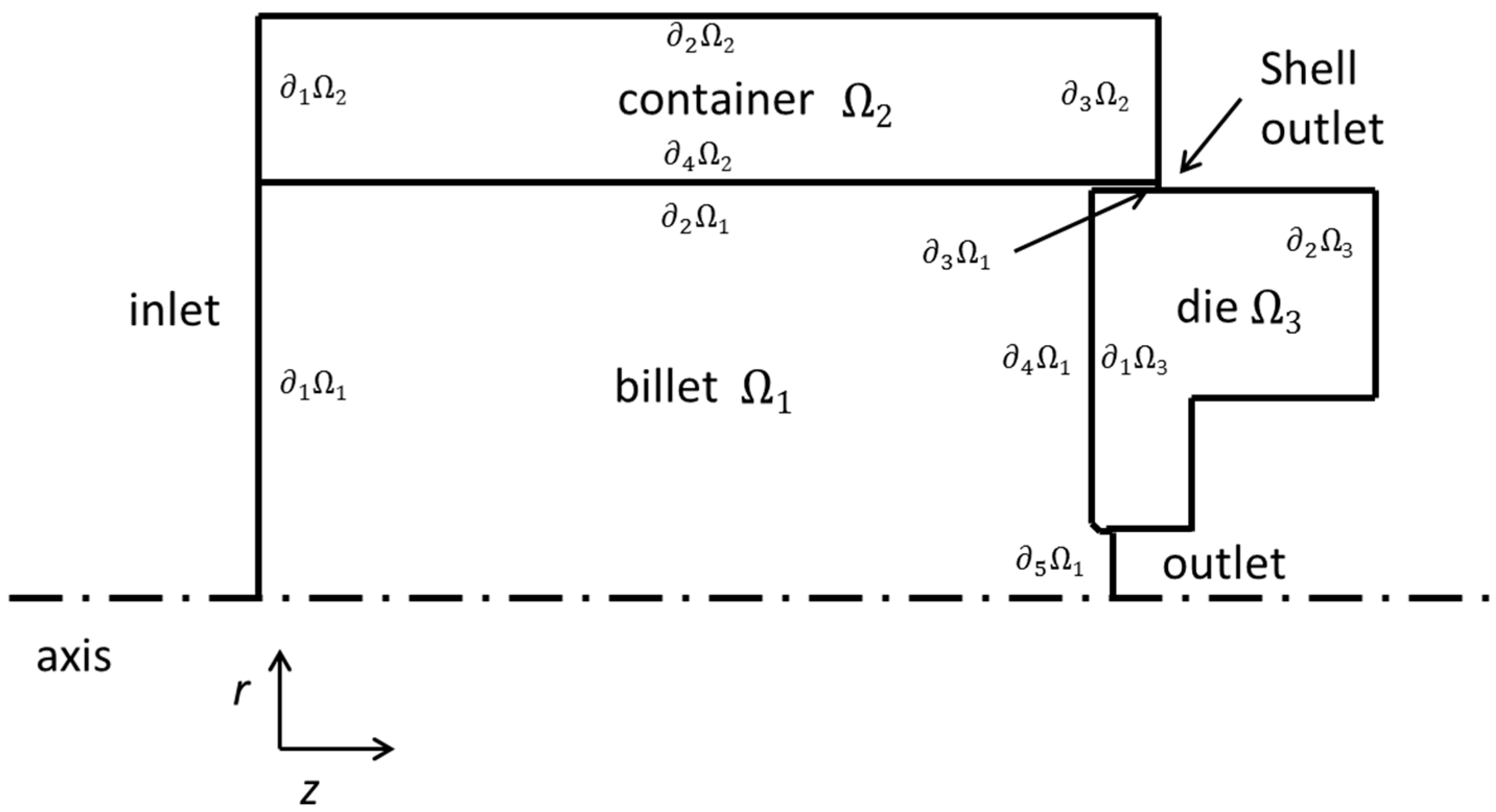
2.1.2. Solution Domain

Equations (1)–(4) are solved in the axisymmetric domain Ω1, depicted in Figure 1 that represents an indirect extrusion process. The process is simulated over a quasi-steady-state window of operation that starts shortly after the press reaches a constant speed and terminates before the ram gets too close to the die. During the steady-state operation all the relevant process quantities (temperature, pressure, etc.) remain constant and therefore, the transient terms on the left hand side (LHS) of (2) and (4) may be ignored.
To simulate the steady-state, a small domain, Ω1, is only required, which captures the flow field near the die. Far from the die, the flow field is uniform. This implies that the billet moves at a constant velocity and does not deform, i.e., at a certain distance from the die, the material is not affected by the process. This is a good approximation for indirect extrusion where the container moves together with the billet and there is virtually no friction between them. If there is significant friction with the container walls, then the entire billet is deformed and the solution domain should contain the entire billet. This is the case for direct extrusion.
The domains Ω2 and Ω3, correspond to the extrusion container and die, respectively. The model includes only the innermost steel layer of the container surface area (liner). The die is modeled as a single uniform item, instead of two distinct steel parts (die & die holder). In Ω3 only the heat transfer Equation (4) is solved, by eliminating all the terms except for the heat conduction term (first term in the RHS), whereas in Ω2 the convective term is retained (second term in the LHS) with uniform horizontal velocity equal to the extrusion speed S, because of the equality between the container and billet speeds.

2.1.3. Boundary Conditions

The conditions imposed on the boundaries of Ω1—denoted ∂iΩ1—are:
Uniform inlet velocity on the left boundary of Ω1,
v r | 1 Ω 1 = 0
v z | 1 Ω 1 = S ,
where v r and v z are the velocity components (radial and axial, respectively) and S is the extrusion speed.
Zero pressure on the outlet:
p | 5 Ω 1 = 0.
The extruded shell sticks to the container walls and therefore, its relative velocity with respect to the container is zero. Since the relative velocity of the container with respect to the die is 0 (radial component) and S (axial component), thereby the velocity of the shell (prescribed at the boundary denoted “shell outlet”) is:
v r | 3 Ω 1 = 0
v z | 3 Ω 1 = S .
It should be noted that by using the boundary conditions (8) and (9), we explicitly restrict any back-extrusion through the gap between the ram and the container. However, we do not observe any back-extrusion in the current process and therefore, Equations (8) and (9) are valid.
Prescribed tangential viscous stress (skin friction) on the die walls is,
τ n t | 4 Ω 1 = f v _   t _ ,
where t _ is the unit tangent vector to the die walls, f is the friction factor derived from a simple model of hydrodynamic lubrication and τ n t is the tangential component of the viscous stress vector ( τ n t = τ n _   t _ = n _   τ _ _   t _ ; n _ is the unit normal vector to the die walls). The lubrication model considers laminar flow between two parallel plates, one of them stationary and the other sliding. Thus, the friction factor is equal to the dynamic viscosity ( μ ) of the lubricant over the size of the gap (L) between the parallel plates.
f = μ L .
For a viscous lubricant such as a graphite paste that is used in the process, a viscosity in the order of 102 Pa s is expected, with a layer thickness in the order of microns. Therefore, the friction factor is expected to be in the order of 108 Ns/m3. It should be noted, however, that f cannot be determined from (11), since the lubrication layer thickness is generally unknown. Instead, we can adjust f to match experimental measurements of the process quantity that is mostly sensitive to it (see Section 3.5), which is the maximum temperature of the extruded product.
Zero tangential viscous stress (slip condition) on the container walls:
τ n t | 2 Ω 1 = 0.
Uniform inlet temperature:
T | 1 Ω 1 = T in .
Temperature continuity on the container and die walls that are in contact with the billet:
T | 2 Ω 1 = T | 4 Ω 2
T | 4 Ω 1 = T | 1 Ω 3 .
Zero conductive heat flux on the outer die walls and on the left/right container walls:
n _ T | 1 Ω 2 = n _ T | 3 Ω 2 = n _ T | 2 Ω 3 = 0.
Heat dissipation on the outer container wall via a simple cooling law:
n _ k T | 2 Ω 2 = h ( T T ) ,
where h is the heat transfer coefficient and T is the ambient temperature; T is prescribed at 27 °C for the present work. It should be noted that the cooling law has little physical meaning here, since ∂2Ω1 is not an outer wall that is exposed to the ambient air, but an inner wall between layers of steel. However, this equation can be used in lieu of a more accurate formulation, with the goal of approximating the average measured temperature of the inner steel liner. In other words, the heat transfer coefficient h is adjusted till the average temperature of Ω2 matches the measured temperature.

2.2. Plastic Stress

The plastic stress in (3) is calculated through the Garofalo equation [18,19]:
A [ sin h ( a σ p ) ] n = Z ,
where A (s−1), a (MPa−1) and n (dimensionless) are parameters that depend on the composition of the material and Z is the Zener–Hollomon parameter [20]:
Z = ε ˙ exp ( Q R T ) ,
where ε ˙ is the equivalent strain rate, Q (J/mol) is the activation energy, R (J/(molK)) is the universal gas constant and T (K) is the absolute temperature. The parameters of Equations (18) and (19) are usually derived from hot torsion experiments with variable temperature and torsion speed [18,19,20,21,22]. By substituting (19) in (18) and solving for σ p , we acquire the plastic stress that is used in (3):
σ p ( ε ˙ ,   T ) = arcsinh ( ( ε ˙ exp ( Q R T ) A ) 1 n ) a
Equation (20) is valid for a single phase alloy. Otherwise, if there are multiple phases with considerably different mechanical properties, e.g., α and β phases of brass, then (20) loses its validity. This happens with the current case of the CW626N alloy, which could be approximated with a CuZn33 brass that also includes other alloying elements. The pure CuZn33 may be an α-brass, but in our case and based on the analysis of the brass billets in production, the equivalent Zn [23] (by virtue of the minor alloying elements and especially Al) is approximately 40%, which corresponds to a binary CuZn40. The equivalent Zn shifts the alloy composition to the regime of (α + β)-brass and as such Equation (20) cannot be used.
Spigarelli et al. [18] suggested that two Garofalo equations could be used instead, one for each brass phase, with a different set of parameters each. The individual plastic stresses, coming from the two equations, contribute to the true plastic stress through a volumetric mixing law:
σ p = ( 1 f β ) σ p , α + f β σ p , β
where f β is the β-phase volume fraction, σ p , α is the α-phase plastic stress and σ p , β is the β-phase plastic stress. The single-phase brass plastic stress ( σ p , α and σ p , β ) is computed using (20), with parameters obtained from hot torsion experiments of single-phase brasses. There is no definite selection of the composition of those brasses, but a reasonable option is to choose single-phase brasses that are close to the transition to dual phase (α + β)-brass. For σ p , β a good selection of pure β-brass is CuZn44 that is marginally close to the transition to dual (α + β)-brass. Similarly for σ p , α a good selection is CuZn36.
We use Equation (21) in the simulations, with σ p , α and σ p , β that correspond to the plastic stresses of α-brass CuZn36 and β-brass CuZn44, respectively. Each individual plastic stress is computed by (20) using the parameters in Table 1 (reported in [19]). The use of a mixing law is essential, because at the process temperature (715 °C) and according to (21), the α-phase is three to four times harder (depending to the strain rate) than the β-phase. This large discrepancy of the mechanical properties between the two phases, reflects on the process parameters as well, especially on the extrusion pressure and temperature. For example, a pure α-phase brass develops an average pressure and maximum temperature during the process, approximately 380 MPa and 820 °C, whereas a pure β-phase develops only 140 MPa and 760 °C (S = 0.015 m/s, Tin = 715 °C).

2.3. Model Assumptions

The following model assumptions were used:
  • Brass phases in the billet are distributed evenly (no spatial variation).
  • There is no phase transition during the extrusion process, i.e., α-brass to β-brass or vice-versa.
  • The temperature of the billet, far from the die (inlet temperature), is uniform.
  • The process is in steady-state regime.
  • Heat generation due to skin friction between the billet and the die is neglected. Heat is only produced due to the deformation of the billet.
  • The alloying elements contribute only to the equivalent Zn.
  • There is no friction between container and billet.
  • The friction between billet and die is based on a simple hydrodynamic lubrication model.

2.4. Reduced Order Model

The CFD model is reduced, using rigorous mathematical techniques (not described here). The reduced order model operates as a replacement of the CFD model and its purpose is to be used by production engineers, without any prior training, neither extensive knowledge of the extrusion process (physics, mathematics, etc.).
The reduced order model is based on the response surface method, initially introduced by Box and Wilson [24] and currently implemented with the DesignXplorer tool (version 18.2, Ansys Inc., Canonsburg, PA, USA) [25]. In essence, it relates output process parameters such as average outlet temperature, extrusion pressure, etc. (in the method nomenclature, these are the response parameters), with input parameters such as the extrusion speed, friction factor, etc. Unlike the CFD model which is computationally intensive and may require execution times from hours to days, the reduced order model, once established, produces results instantaneously and can be used to extensively investigate the process characteristics with respect to several input parameters (see Section 3.6). It should be noted, however, that the establishment of the reduced order model requires design of (computational) experiments (DoE) [25,26] and as such, it is by itself a computationally intensive task.

2.5. Process Parameters

The process parameters are separated in input parameters (imposed on the process, e.g., extrusion speed), and output parameters (dictated by the process and dependent on the input parameters, e.g., average temperature of the extruded product).

2.5.1. Input Parameters

The considered input parameters are shown in Table 2. The extrusion speed, S, is directly set by the control system of the hydraulic press. The inlet temperature, Tin, is equal to the temperature of the billet (considered uniform) right before the start of the extrusion process. It should be noted that currently there are no means to determine whether Tin is in fact equal to the temperature of the billet before it enters the container, e.g., there may be a significant decrease and non-uniformity of the billet temperature if it stays idle in the container.
The β-phase volume fraction, f β , is determined by the equivalent Zn of the billet. The simplest approach to calculate f β , would be to assume phase equilibrium at Tin and consult the binary Cu–Zn phase diagram. Given the equivalent Zn of the brass used in the process (~40%), the volume fraction of β-phase at the extrusion temperature is approximately 0.5.
In the current model, there is no method to determine h and therefore, it was approached in a different manner, described in Section 2.1.3: h was adjusted until the average temperature of the container liner reaches the measured temperature (measurements performed with an optical pyrometer); for this case study the average temperature is ~550 °C and h was determined (by trial-and-error) to about 1.7 W (m2 K).
The friction factor, f, is yet another unknown input parameter that depends on the lubricant type and may be determined using an approach similar to that used for the determination of h. f has a strong impact on the temperature of the extruded product (see Section 3.5) and, thus, it may be adjusted until the calculated average temperature at the outlet of the container, reaches the measured temperature.

2.5.2. Output Parameters

The considered output parameters are shown in Table 3. In order to convert the pressure of the hydraulic press (bar) to the pressure inside the container (extrusion pressure in Pa), it has to be multiplied by 1.68 × 10⁶; this factor is calculated from the specifications of the hydraulic press.

2.6. Thermo-Physical Properties

The thermo-physical properties of the model are shown in Table 4 [27].

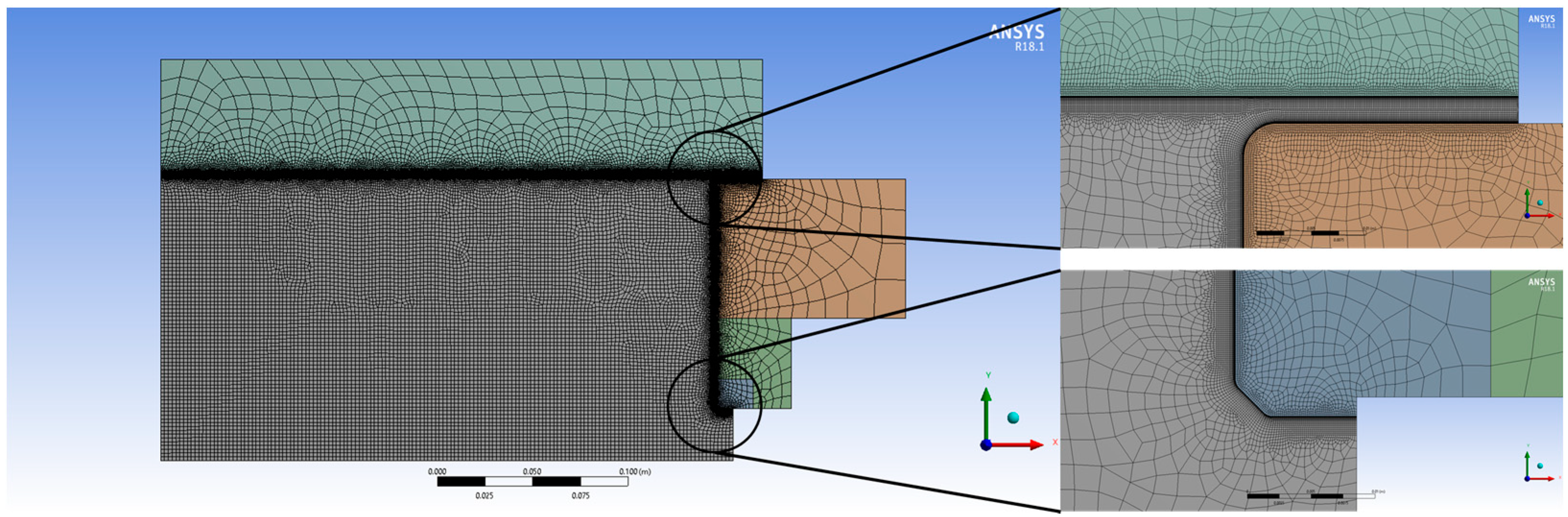
2.7. Mesh Sensitivity—Model Validity

The utilized mesh is shown in Figure 2. It consists of ~100,000 elements with boundary layers of smaller elements at the container and die walls, in order to resolve the steep solution profiles (temperature, velocity, etc.), especially near the abrupt geometrical features of the die. The current mesh is excessively refined, because the computational cost for the solution of a 2D problem is not considerable, even for very refined meshes. In fact, by coarsening the mesh more than half its original size (~40,000 elements), the relative difference of the calculated average pressure was less than 5% and the absolute difference of the calculated maximum and average temperatures of the billet was less than 1 °C. Therefore, we deem the solution independent of the mesh for the purposes of this work.
The accuracy of the model is examined with the aid of ongoing production trials. At the current stage we are able to successfully reproduce the actual hydraulic pressure during the steady-state operation. To elaborate, experiments were performed (Table 5), during the normal production process that involved the measurement of the container liner temperature and the billet temperature, before and after the extrusion. With the establishment of these temperatures that provide the average temperature of important components (billet: 715 °C, liner: 550 °C), along with the steady extrusion speed (1.5 cm/s) and the brass composition, we calculate the hydraulic pressure, which turns out to be identical to the actual one (approximately 160 bar).
The validation of the model will continue using measurements from production, with variations of extrusion speed and/or brass composition.

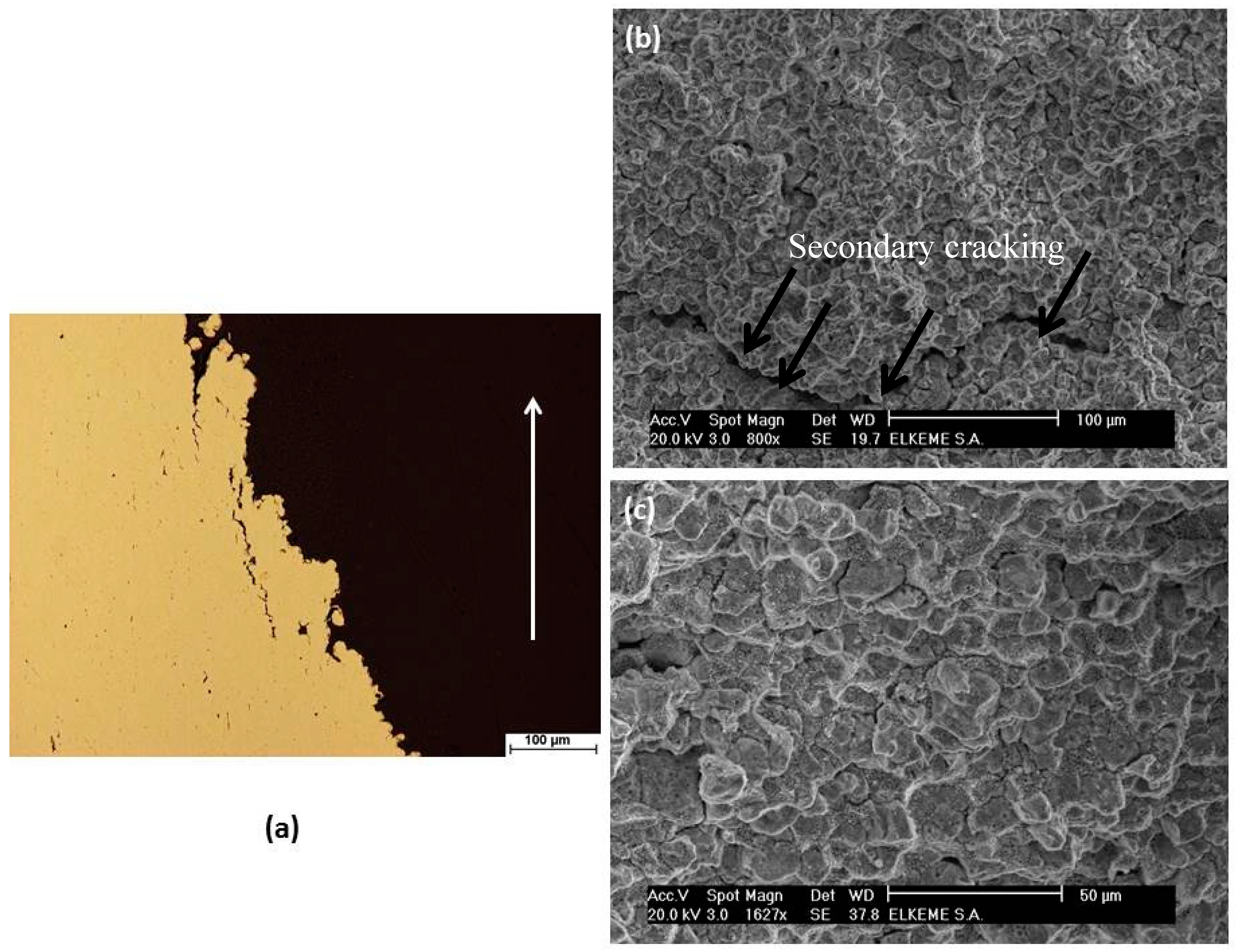
2.8. Experimental Characterization—Metallography and Fractography

Metallographic characterization of a typical dual-phase (α + β) brass was conducted on transverse cross-sections, after wet grinding up to 1200 grit SiC paper, followed by fine polishing using diamond and silica suspensions and finishing with ethanol and compressed-air drying. Subsequently, immersion chemical micro-etching, for approximately 5 s at room temperature, was performed using FeCl3-based solution (Merck, Darmstadt, Germany) according to the ASTM E407 standard. Light optical metallography was performed using a Nikon Epiphot 300 (Nikon, Tokyo, Japan) inverted optical microscope using image analysis software, Image Pro Plus Version 7.0 (Rockville, MD, USA) for phase (area) fraction measurements. High-magnification fracture surface observations, utilizing a FEI XL40 SFEG scanning electron microscope (FEI, Eindhoven, The Netherlands), were realized using secondary electron (SE) imaging under 20 kV accelerating voltage.

3. Results and Discussion
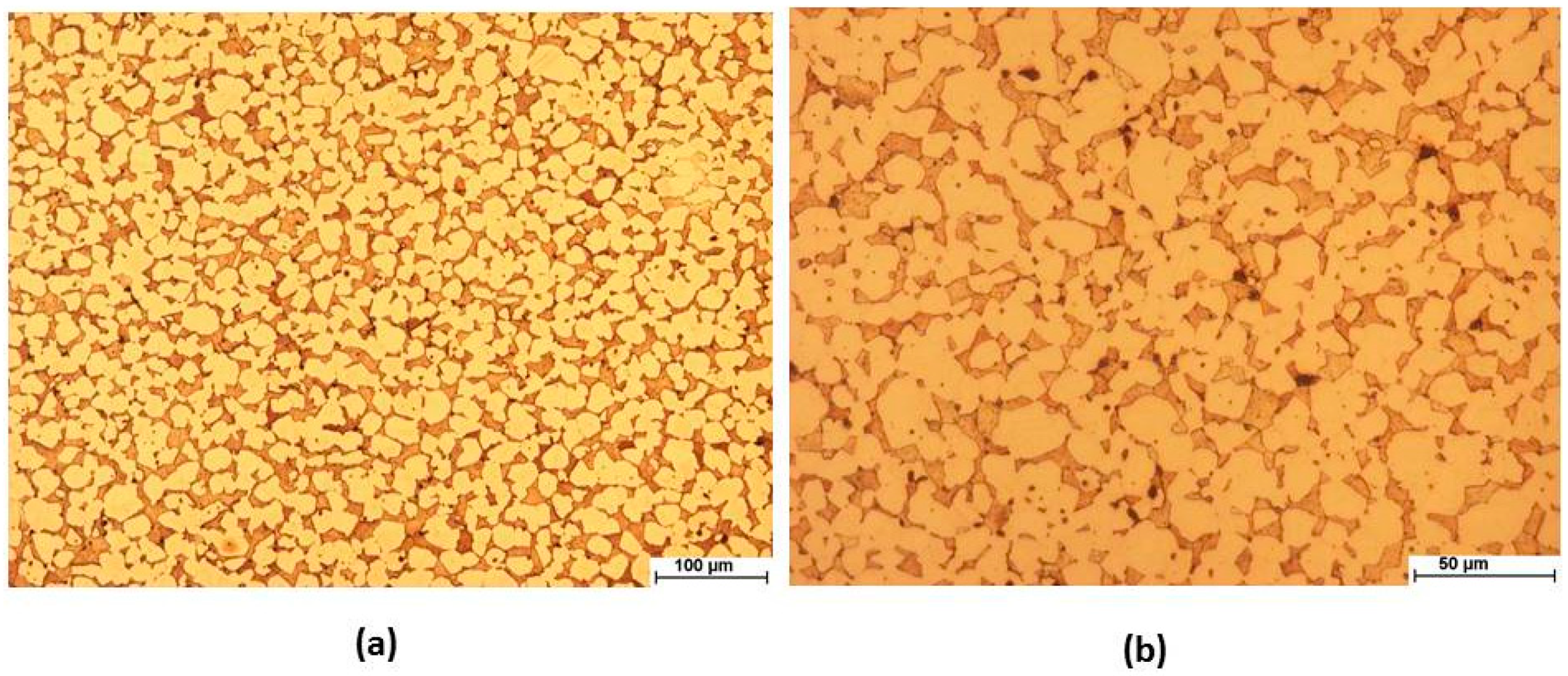
3.1. Microstructure

A typical dual phase structure of a common dual phase brass alloy is shown in Figure 3. The phase structure consisted of approximately 65% α-phase and 35% β-phase. The α-phase represents the Cu solid solution with Zn (exhibiting a face-centered-cubic crystal lattice), while β-phase is the ordered non-stoichiometric intermetallic compound CuZn possessing a body-centered-cubic (bcc) lattice. Lead particles (seen as black-dots of size of 1 μm approximately) are well distributed mainly in the α/β interface areas, which act as high surface energy positions. The phase structure for these alloys depends on alloy chemical composition as well as on casting and hot working conditions, i.e., casting temperature, casting speed, extrusion temperature and cooling rate. Pb-particle size and distribution is predominantly influenced by casting and solidification conditions, while the phase structure, such as volume fraction of β-phase and grain size, is influenced mainly by hot extrusion conditions. The presence of β-phase significantly affects the mechanical behavior and machinability of the extruded brass [5,28].

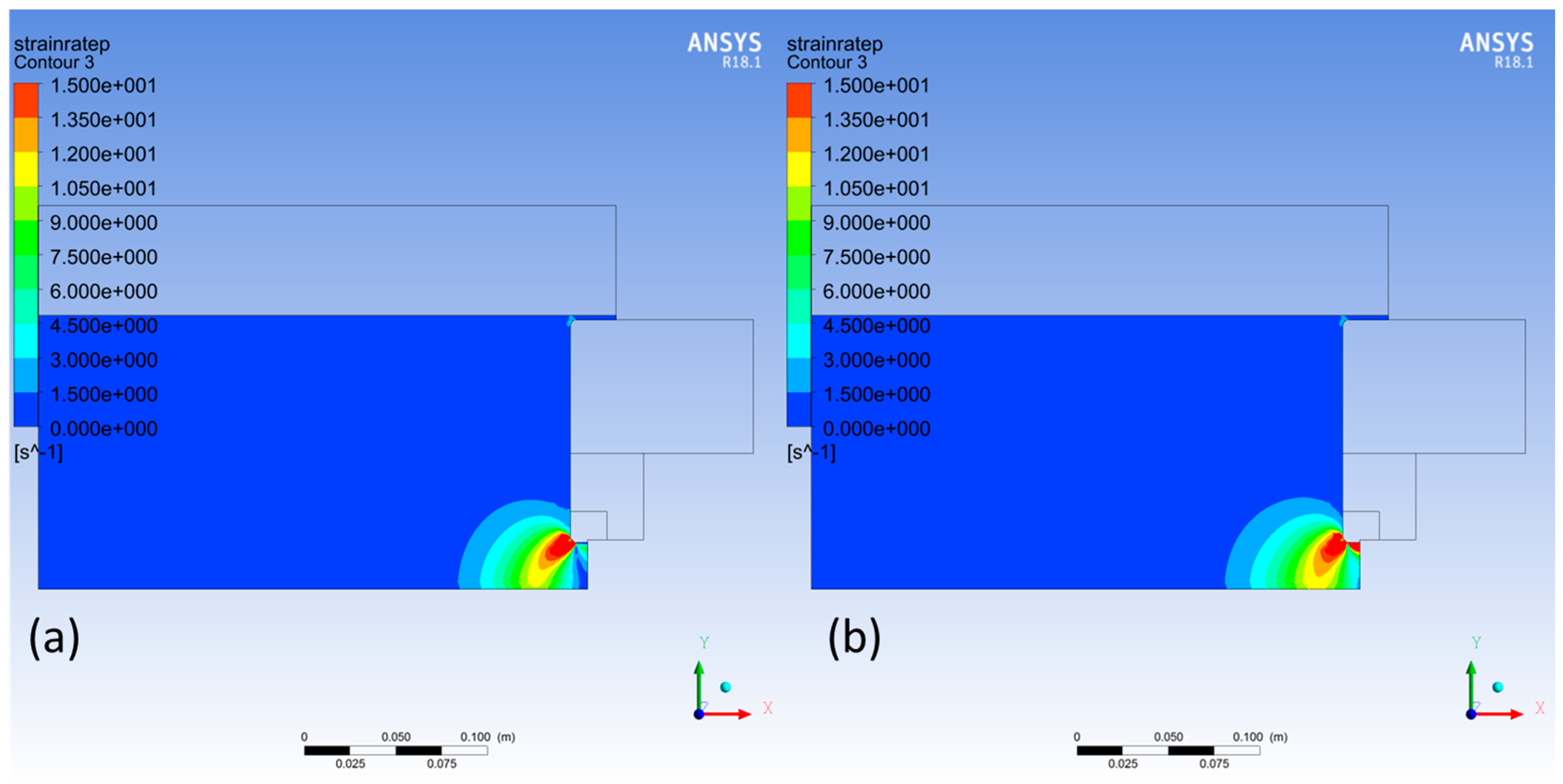
3.2. Equivalent Strain Rate
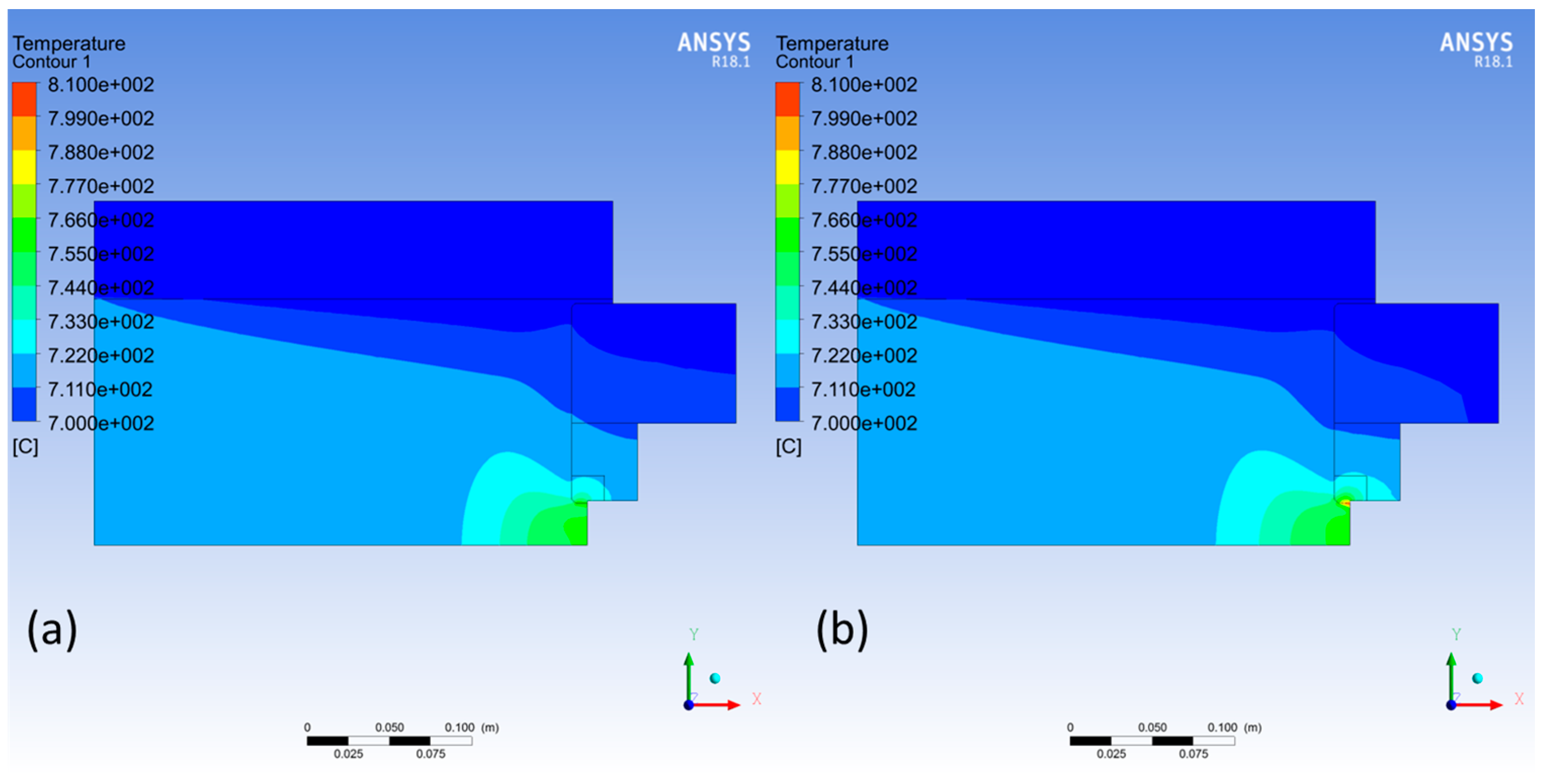
An important calculated quantity that affects the process characteristics and especially the extrusion pressure and the generation of heat due to deformation, is the equivalent strain rate (appears in Equations (2)–(4)). The equivalent strain rate has a typical profile shown in Figure 4a. The strain rate is large near the die and especially at locations, where there is an abrupt change of the die geometry (edges and slopes). Also, in cases where there is a high friction factor on the die walls, we observe large strain rates on the horizontal die walls near the outlet (Figure 4b). This occurs because the extruded metal sticks to the die, thus straining the metal layers adjacent to the die walls. The locally high strain rates near the die are also responsible for elevating the temperature considerably at the outer layers of the extruded product (see Section 3.3). The phase structure of the reference dual phase alloy consists of 65% α and 35% β under room temperature conditions. The β-phase fraction ( f β ) is taken to be approximately equal to 0.5, which corresponds to an equi-volume phase structure, consisting of 50% α and 50% β at the extrusion temperature (Tin = 715 °C).

3.3. Temperature

The temperature of the billet decreases near the container walls, due to the conduction of heat through the steel liner, but also increases near the die, due to the plastic deformation energy that is converted to heat (see heat transfer Equation (4)). The model shows a significant increase of temperature at the outlet—compared to the inlet temperature—in the neighborhood of 50 °C (average temperature of the extruded product).
The temperature increases towards the outlet (Figure 5a), where the equivalent strain rate is large, regardless of the friction of the billet with the die walls. If however, the friction factor is large, then the local strain rate is large near the horizontal die walls as well (Figure 4b), which consequently translates to the formation of hot spots in the outer layers of the extruded product (Figure 5b). The temperature of the hot spots may surpass the inlet temperature by more than 100 °C, depending on the process parameters (extrusion speed, friction factor, etc.).
This may be detrimental to the process, because a very high temperature at the surface of the extruded product may cause severe defects, such as surface cracks (hot shortness); see [29] and Section 3.7.

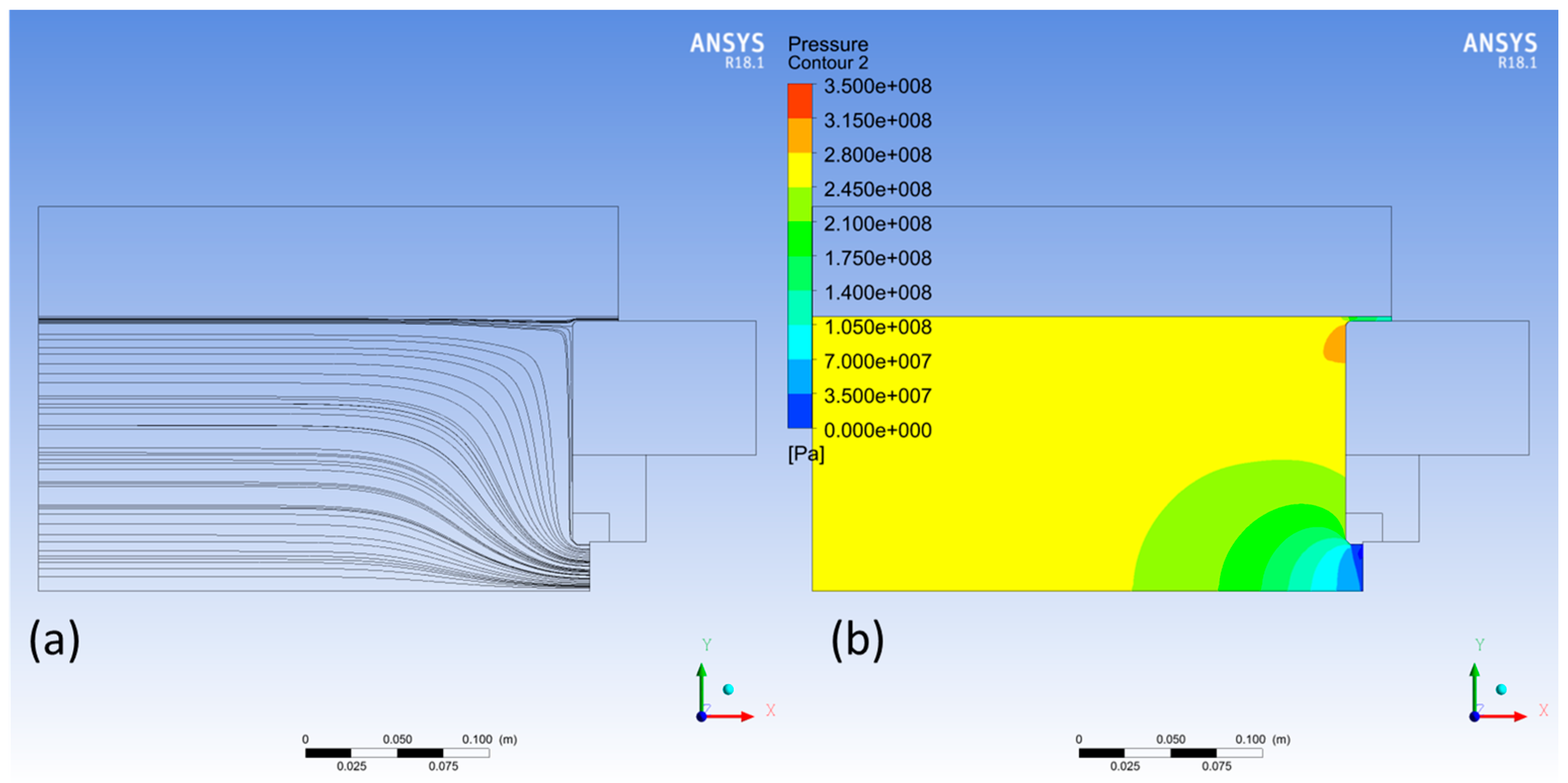
3.4. Pressure/Flow Profile

A typical flow profile is shown in Figure 6a. The streamlines begin to converge towards the outlet at about ~15 cm from die. This suggests that the billet moves as an unyielding solid body, until it reaches a threshold at a certain distance before the die. This justifies our decision to simulate the process only in a small computational domain containing only the region beyond the threshold.
Moreover, streamlines diverge near the shell outlet, forming a flow stagnation point on the surface of the die holder, which translates in a localized pressure increase (Figure 6b). Far from the die, the pressure is virtually uniform and equal to the extrusion pressure, which as we discussed above is related to the measured pressure of the hydraulic press (see Section 2.5.2).

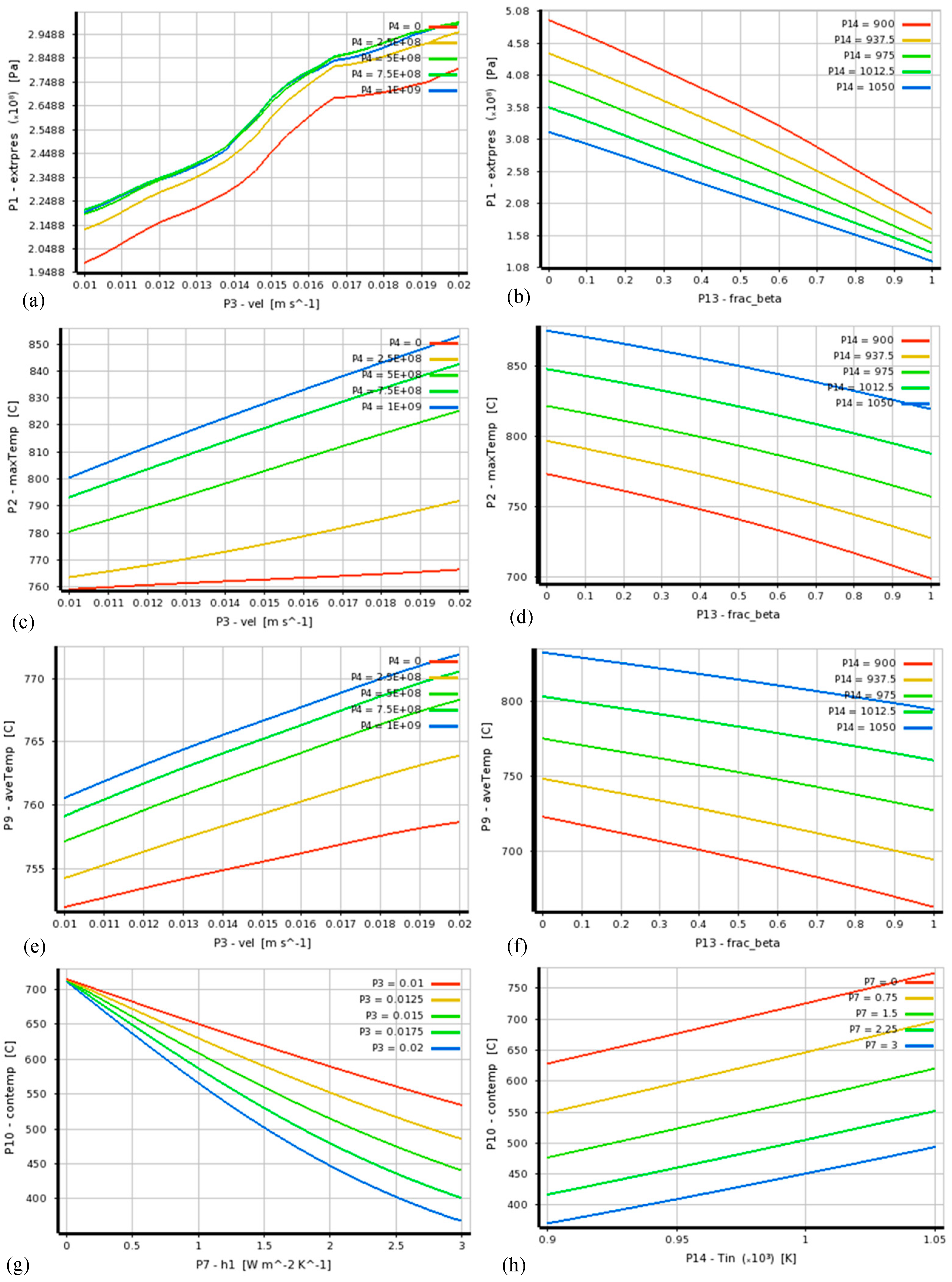
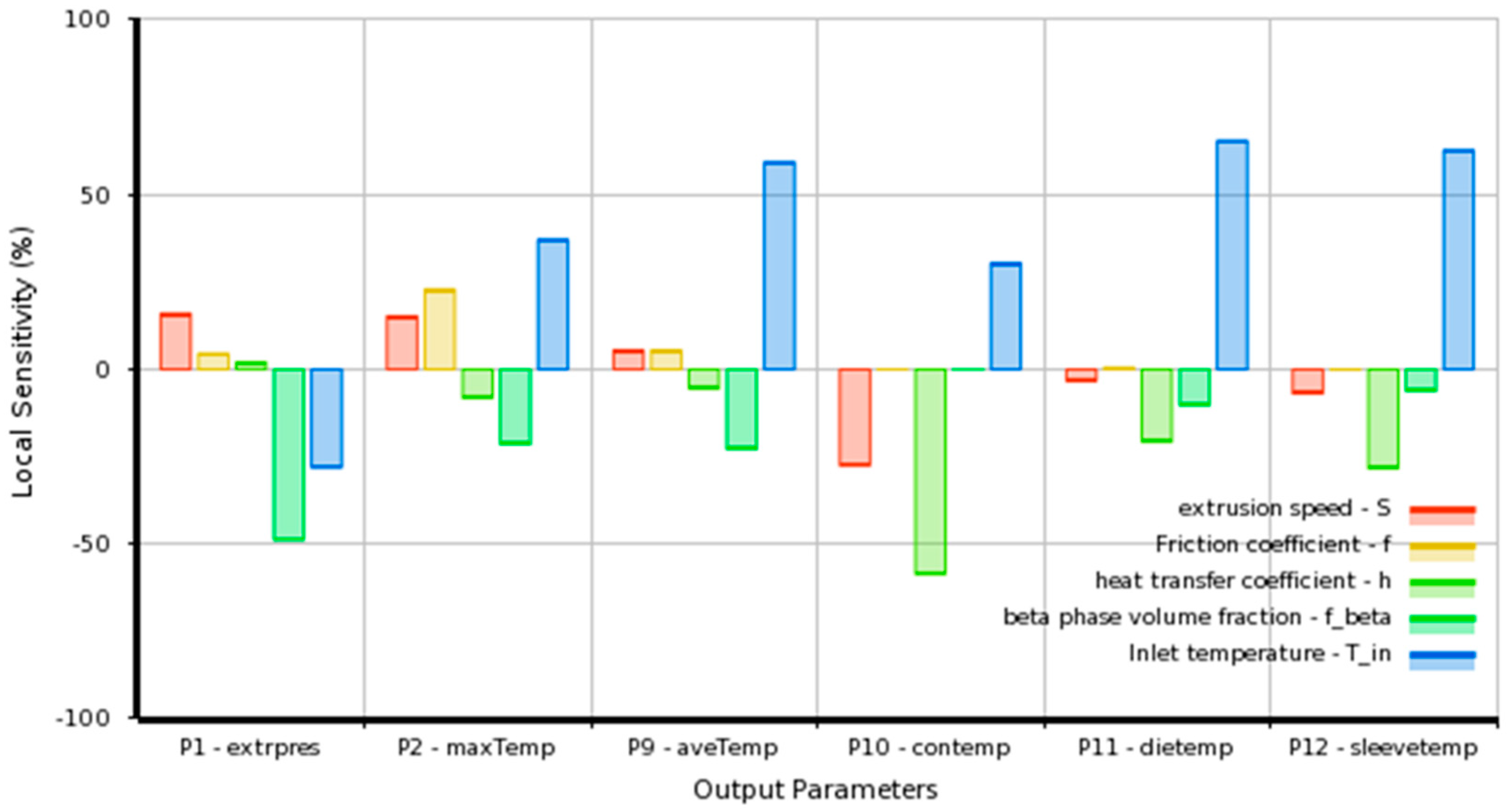
3.5. Sensitivity Analysis

The sensitivity of the output parameters to changes of the input parameters is presented in Figure 7. Each bar represents the change of a single output parameter with respect to the change of a single input parameter for a given interval, e.g., we allow that the extrusion speed goes from 0.01 to 0.02 m/s. For that change of extrusion speed, the extrusion pressure increases by an amount represented by the first red bar. On the other hand, we allow that fβ changes from 0 to 1, which has the effect of lowering the extrusion pressure by an amount represented by the first inverted green bar (negative effect). The green bar is longer than the red bar and therefore, by going from pure α-phase to pure β-phase, the impact on the extrusion pressure is larger than by increasing the speed from 0.01 to 0.02 m/s. The intervals of the input parameters that are used for the construction of the chart in Figure 7, are shown in Table 6.

3.6. Parametric Study

The reduced order model enables a very extensive parametric study. In Figure 8 selected charts of the process output parameters vs. input parameters were presented, produced by the reduced order model. These charts encapsulate the importance of the reduced order model, since we can acquire results on-demand without using a complex numerical model. For example, let us consider an increase of extrusion speed for the sake of increasing the production capacity. The increase is only modest (~13%), going from 1.5 cm/s to 1.7 cm/s. From Figure 8a,c, using the default parameter values, we gather that the speed increase results in ~8% increase of the extrusion pressure and the increase of the maximum temperature by ~10 °C. Another example would be the reduction of the preheating furnace temperature down to 664 °C from 715 °C. By consulting Figure 8b, we find that this alteration results in the increase of the extrusion pressure up to 310 MPa and therefore 184 bar hydraulic pressure.

3.7. Phenomenological Aspects of Flow-Induced Extrusion Failures

High and/or localized impurity levels may result in cracking and discontinuities after extrusion. Bismuth (Bi) in the alloy can lead to the formation of brittle inter-granular films that aggravate hot shortness and adversely affect the hot workability of the alloy. On the other hand, excess antimony (Sb) impairs cold workability [30,31].
A back-defect that generally appears as a hole at the end of the extruded rod results from a combination of the metal flow-pattern and the introduction of surface oxides into the interior of the rod [29]. The flow pattern established by the differences in flow rates draws surface oxides into the center of the rod and the successive metal layers cannot weld together. The lack of “welding” between the mating surfaces results in the formation of such discontinuities and central rod defects.
Removing a certain length from the end of the extruded rod restricts the inheritance of this defect to the downstream processes and eventually to the final product. The back-defect is not common for indirect extrusion processes.
Hot-shortness failures appear in the form of surface cracks along the length of the extrusion. Hot-shortness results from overheating due to the high localized temperature (hot-spots), as a result of billet/die friction. This phenomenon raises the metal temperature to the point where localized regions of segregation may melt or become hot-short. The frictional heat dissipated during extrusion may also cause hot-tears on the metal surface. The surfaces of such tears oxidize and do not re-join during the metal processing operations. The non-bonded regions lead to further cracking or delaminations.
Other studies highlight the importance of the average shear strain rate criterion during the extrusion of brass (e.g., CuZn30), see Ref. [31]. Exceeding a certain threshold (e.g., 0.9 s−1 for CuZn30), the risk of transverse cracking is significant, as it can be illustrated by the relevant extrusion ratio-speed process curves that show a characteristic safe/failure boundary. A decrease in the extrusion temperature and in the extrusion speed will generally eliminate defects introduced due to hot shortness phenomena that result in intergranular fractures [12,32,33]. Typical intergranular fracture morphology of brass rod, induced due to high speed extrusion which resulted in overheating is illustrated in Figure 9. The presence of Pb might exaggerate the hot-shortness phenomena that are a result of localized melting and subsequent tearing due to “internal” liquid metal embrittlement. The presence of Pb particles could lead to the generation of voids, followed by growth, realized by an adsorption-induced decohesion, or dislocation emission process that will finally result in coalescence and necking (as is diligently outlined in Ref. [34]).
The utilization of the CFD-based extrusion model is expected to become a plant-based practice aiming to predict and prevent extrusion temperature rises that lead to the aggravation of hot-shortness/overheating-related defects formation. This is a preliminary step that will find promising applications only following systematic validation in actual production.

4. Conclusions

A CFD-based model of dual phase brass extrusion was presented that is based on constitutive laws and the Zener–Hollomon parameter that connects plastic stress and strain rate. The main scope of the present research work is the investigation of the metal-flow pattern during indirect extrusion, and the calculation of the main output parameters such as extrusion pressure and temperature. The main results of the present study can be summarized as follows:
(1) A reduced order model was attempted, which is an approximation of the CFD model that relates the process input and output parameters, such as extrusion pressure vs speed (velocity). The reduced order model can be readily used by plant production personnel, since it can be embedded in a simple spreadsheet.
(2) The CFD model accommodates the rigorous theory of plastic deformation, and takes also into account the different plastic responses during extrusion of the two phases in equilibrium (α and β).
(3) The CFD model predicts the formation of hot-zones near the die (due to the local high strain rates), which may induce severe defects in the final product.
Knowledge of the extrusion metal flow pattern, as this is derived solving the constitutive laws together with the ad hoc assumption of dual phase plastic stress behavior (“rule of mixtures”) and its relation to viscosity, could become a promising first step for the development of an integrated defect/failure prognostic tool that will effectively assist in the improvement of the product and process quality. Further adjustment/validation of the CFD model is required, based on crucial plant information that will associate the model output parameters and the formation of critical defects.

Author Contributions

Conceptualization and Simulation, G.P.; Supervision, I.C.; Project Consulting, Review and Paper Editing, G.A.P.

Funding

This research received no external funding.

Acknowledgments

The authors wish to express special thanks to the Management and Quality Division of FITCO Metal Works S.A. for the continuous support assisting in the project’s realization and completion and for granting permission for the current publication.

Conflicts of Interest

The authors declare no conflict of interest.

Appendix A. Relationship between Plastic Stress and Viscosity

The foundation of the approach that converts the plastic stress of a yielded solid material to an equivalent viscosity—with the purpose of using fluid dynamics to simulate the extrusion of a solid material—is based on the von Mises yield criterion. According to this, a solid material yields (i.e., flows plastically), when a function of the second invariant of the deviatoric stress tensor, referred to as equivalent von Mises stress, reaches a critical value, referred to as yield stress. Therefore, when the solid material yields, the equivalent von Mises stress is equal to the yield stress, or according to our notation, it is equal to the plastic stress:
σ v = σ y σ p ,
where σ v is the equivalent von Mises stress and σ y is the yield stress, which is identical to the plastic flow stress, σ p .
The von Mises theory has two fundamental quantities that describe the stresses and strain rates in solids under multiaxial loading conditions. Those are the equivalent stress, σ v (described above), and the equivalent strain rate, ε ˙ . They are formulated as [35]:
σ v = 3 2 τ _ _ τ _ _
and
ε ˙ = 2 3 ε ˙ _ _ ε ˙ _ _ ,
where τ _ _ is the deviatoric stress tensor, also called viscous stress tensor in the field of fluid dynamics and ε ˙ _ _ is the rate-of-strain tensor. It should be noted that σ v and ε ˙ come from more general relations, involving the second invariant of their corresponding tensors, e.g., (A2) comes from σ v = 3 J 2 , where J 2 is the second invariant of τ _ _ . This yields σ v = 3 [ 1 2 tr ( τ _ _ 2 ) ] , given that τ _ _ is traceless ( tr ( τ _ _ ) = 0 ), and hence σ v = 3 2 τ _ _ τ _ _ . A similar procedure is applied for (A3) also, however, ε ˙ _ _ is not generally traceless and as such (A3) would not hold. However, under the constraint of incompressibility (Equation (1)), tr ( ε ˙ _ _ ) = 0 and (A3) is valid.
We use a general equation from fluid dynamics, connecting τ _ _ with ε ˙ _ _ [16] that reads:
τ _ _ = 2 μ ε ˙ _ _ ,
where μ is the dynamic viscosity. The substitution of (A4) in (A2), yields:
σ v = 6 μ 2 ε ˙ _ _ ε ˙ _ _ .
The combination of (A5) and (A3) yields:
σ v = 3 μ ε ˙ .
And finally the introduction of (A1) into (A6), yields the expression for the viscosity,
μ = σ p 3 ε ˙

References

  1. Kuyucak, S.; Sahoo, M. A review of the machinability of copper-base alloys. Can. Met. Q. 1996, 35, 1–15. [Google Scholar] [CrossRef]
  2. Pantazopoulos, G. Leaded brass rods C38500 for automatic machining operations. J. Mater. Eng. Perform. 2002, 11, 402–407. [Google Scholar] [CrossRef]
  3. Gane, N. The effect of lead on the friction and machining of brass. Philos. Mag. 1981, 43, 545–566. [Google Scholar] [CrossRef]
  4. Garcia, P.; Rivera, S.; Palacios, M.; Belzunce, J. Comparative study of the parameters influencing the machinability of leaded brasses. Eng. Fail. Anal. 2010, 17, 771–776. [Google Scholar] [CrossRef]
  5. Pantazopoulos, G.; Toulfatzis, A. Fracture modes and mechanical characteristics of machinable brass rods. Met. Microstruct. Anal. 2012, 1, 106–114. [Google Scholar] [CrossRef]
  6. Toulfatzis, A.; Pantazopoulos, G.; Paipetis, A. Fracture behavior and characterization of lead-free brass alloys for machining applications. J. Mater. Eng. Perform. 2014, 23, 3193–3206. [Google Scholar] [CrossRef]
  7. Toulfatzis, A.; Pantazopoulos, G.; Paipetis, A. Microstructure and properties of lead-free brasses using post-processing heat treatment cycles. Mater. Sci. Technol. 2016, 32, 1771–1781. [Google Scholar] [CrossRef]
  8. Toulfatzis, A.; Pantazopoulos, G.; Paipetis, A. Fracture mechanics properties and failure mechanisms of environmental-friendly brass alloys under impact, cyclic and monotonic loading conditions. Eng. Fail. Anal. 2018, 90, 497–517. [Google Scholar] [CrossRef]
  9. Toulfatzis, A.; Pantazopoulos, G.; David, C.; Sagris, D.; Paipetis, A. Final heat treatment as a possible solution for the improvement of machinability of lead-free brass alloys. Metals 2018, 8, 575. [Google Scholar] [CrossRef]
  10. Toulfatzis, A.I.; Pantazopoulos, G.A.; Besseris, G.J.; Paipetis, A.S. Machinability evaluation and screening of leaded and lead-free brasses using a non-linear robust multifactorial profiler. Int. J. Adv. Manuf. Technol. 2016, 86, 3241–3254. [Google Scholar] [CrossRef]
  11. Toulfatzis, A.; Pantazopoulos, G.; David, C.; Sagris, D.; Paipetis, A. Machinability of eco-friendly lead-free brass alloys: Cutting-force and surface-roughness optimization. Metals 2018, 8, 250. [Google Scholar] [CrossRef]
  12. Pantazopoulos, G. A review of defects and failures in brass rods and related components. Pract. Fail. Anal. 2003, 3, 14–22. [Google Scholar] [CrossRef]
  13. Valberg, H.S. Applied Metal Forming—Including FEM Analysis; Cambridge University Press: Cambridge, UK, 2010. [Google Scholar]
  14. Bozzi, S.; Vedani, M.; Lotti, D.; Passoni, G. Extrusion of aluminium hollow pipes: Seam weld quality assessment via numerical simulation. Met. Sci. Technol. 2009, 27, 20–29. [Google Scholar]
  15. Mitsoulis, E. Flows of viscoplastic materials: Models and computations. Rheol. Rev. 2007, 2007, 135–178. [Google Scholar]
  16. Bird, R.B.; Stewart, W.E.; Lightfoot, E.N. Transport Phenomena, 2nd ed.; Wiley: Hoboken, NJ, USA, 2002. [Google Scholar]
  17. Schmitter, E.D. Modelling massive forming processes with thermally coupled fluid dynamics. In Proceedings of the COMSOL Multiphysics User’s Conference, Bostion, MA, USA, 23–25 October 2005. [Google Scholar]
  18. Spigarelli, S.; El Mehtedi, M.; Cabibbo, M.; Gabrielli, F.; Ciccarelli, D. High temperature processing of brass: Constitutive analysis of hot working of Cu–Zn alloys. Mater. Sci. Eng. A 2014, 615, 331–339. [Google Scholar] [CrossRef]
  19. Spigarelli, S.; El Mehtedi, M.; Cabibbo, M. Characterization of Hot Deformation of CW602N Brass. Acta Phys. Pol. 2015, 128, 726–729. [Google Scholar] [CrossRef]
  20. Pernis, R.; Kasala, J.; Boruta, J. High temperature plastic deformation of CuZn30 brass—Calculation of the activation energy. Kov. Mater. 2010, 48, 41–46. [Google Scholar] [CrossRef]
  21. Yang, L.-C.; Pan, Y.-T.; Chen, I.-G.; Lin, D.-Y. Constitutive relationship modeling and characterization of flow behavior under hot working for Fe–Cr–Ni–W–Cu–Co super-austenitic stainless steel. Metals 2015, 5, 1717–1731. [Google Scholar] [CrossRef]
  22. Orman, L. Tensile Behaviour of Alpha Brasses at Elevated Temperature. Master’s Thesis, Department Metallurgical Engineering, University of British Columbia, Salt Lake City, UT, USA, 1982. [Google Scholar]
  23. Gulyaev, A.P. Physical Metallurgy; MIR Publishers: Moscow, Russia, 1980; Volume 2. [Google Scholar]
  24. Box, G.E.P.; Wilson, K.B. On the experimental attainment of optimum conditions (with discussion). J. R. Stat. Soc. Ser. B 1951, 13, 1–45. [Google Scholar]
  25. Ansys Inc. DesignXplorer User’s Guide; Ansys Inc.: Canonsburg, PA, USA, 2017. [Google Scholar]
  26. Fluent, A. Theory Guide; Ansys Inc.: Canonsburg, PA, USA, 2017. [Google Scholar]
  27. Valencia, J.J.; Quested, P.N. Thermophysical properties. In ASM Handbook; ASM International: Novelty, OH, USA, 2008; Volume 15, pp. 468–481. [Google Scholar]
  28. Pantazopoulos, G.; Vazdirvanidis, A. Characterization of microstructural aspects of machinable α-β phase brass. Microsc. Anal. 2008, 22, 13–16. [Google Scholar]
  29. Laue, K.; Stenger, H. Extrusion—Processes Machinery, Tooling; ASM International: Novelty, OH, USA, 1981. [Google Scholar]
  30. Higgins, R. Engineering Metallurgy-Applied Physical Metallurgy, 6th ed.; Edward Arnold: London, UK, 1998. [Google Scholar]
  31. Pernis, R.; Kasala, J.; Pernis, I. Surface defects of brass bars. In Proceedings of the International Conference “Metal 2011”, Brno, Czech Republic, 18–20 May 2011. [Google Scholar]
  32. Pantazopoulos, G.; Vazdirvanidis, A. Failure analysis of a fractured leaded-brass (CuZn39Pb3) extruded hexagonal rod. J. Fail. Anal. Prev. 2008, 8, 218–222. [Google Scholar] [CrossRef]
  33. Pantazopoulos, G.; Vazdirvanidis, A. Fracture analysis and embrittlement phenomena of machined brass components. Procedia Struct. Integr. 2017, 5, 476–483. [Google Scholar] [CrossRef]
  34. Lynch, S.P. Failures of structures and components by metal-induced embrittlement. J. Fail. Anal. Prev. 2008, 8, 259–274. [Google Scholar] [CrossRef]
  35. Sugimoto, M.; Igaki, H.; Saito, K. Equivalent stress (rate) and equivalent strain rate for work-hardening materials: Theory of anisotropic plasticity based on maximum shear stress hypothesis. Trans. Jpn. Soc. Mech. Eng. 1973, 39, 1164–1174. [Google Scholar] [CrossRef]
Figure 1. Solution domain for the steady-state indirect extrusion problem. Only a small segment of the billet near the die is considered, where the effects of the process are significant; far from the die the billet is relatively unaffected by the process. The domain consists of three subdomains, Ω1, Ω2 and Ω3 (billet, container and die respectively), with their corresponding boundaries denoted as ∂iΩ1, ∂iΩ2 and ∂iΩ3.
Metals 08 01043 g001
Figure 2. Computational mesh consisting of ~100,000 elements. The mesh is refined near the container and die walls, with 20 layers that span ~1.5 mm; the wall adjacent layer has a thickness of 10 μm.
Metals 08 01043 g002
Figure 3. (a) Optical micrograph of the microstructure of a typical dual-phase brass on transverse section. (b) Detail of (a). Bright areas represent α-phase and dark areas represent β-phase. In (a) there is an appreciable amount of Pb particles, which appeared as black dots. Immersion etching in FeCl3-based solution.
Metals 08 01043 g003
Figure 4. Contours of the equivalent strain rate (values larger than 15 s−1 are clipped to the red color contour). (a) Solution with no friction f = 0 Ns/m3, S = 1.5 cm/s, fβ = 0.5, Tin = 715 °C, h = 1.7 W/(m2 K). (b) Solution with friction f = 5 × 10⁸ Ns/m3, S = 1.5 cm/s, fβ = 0.5, Tin = 715 °C, h = 1.7 W/(m2 K).
Metals 08 01043 g004
Figure 5. Contours of temperature (values smaller than 700 °C are clipped to the blue color contour). (a) Solution with no friction f = 0 Ns/m3, S = 1.5 cm/s, fβ = 0.5, Tin = 715 °C, h = 1.7 W/(m2 K). (b) Solution with friction f = 5 × 10⁸ Ns/m3, S = 1.5 cm/s, fβ = 0.5, Tin = 715 °C, h = 1.7 W/(m2 K). Notice the formation of a small hot spot—due to high friction—near the outlet and on the outer layer of the extruded product.
Metals 08 01043 g005
Figure 6. (a) Streamlines. (b) Pressure contours. Parameter values: f = 5 × 10⁸ Ns/m3, S = 1.5 cm/s, fβ = 0.5, Tin = 715 °C, h = 1.7 W/(m2 K).
Metals 08 01043 g006
Figure 7. Sensitivity chart of the output parameters (designated by column—horizontal axis) with respect to the input parameters (designated by color bars). The analysis is performed in the neighborhood of a reference point with input parameter values: f = 5 × 10⁸ Ns/m3; S = 1.5 cm/s, fβ = 0.5, Tin = 715 °C, h = 1.7 W/(m2 K).
Metals 08 01043 g007
Figure 8. Process charts showing the dependence of the process output parameters on the input parameters. (a) Extrusion pressure (P1) vs. extrusion speed (S). (b) Extrusion pressure (P1) vs. β-phase fraction (fβ). (c) Max. extrusion temperature (P2) vs. extrusion speed (S). (d) Max. extrusion temperature (P2) vs. β-phase fraction (fβ). (e) Average extrusion temperature (P9) vs. extrusion speed (S). (f) Average extrusion temperature (P9) vs. β-phase fraction (fβ). (g) Container temperature (P10) vs. heat transfer coefficient (h). (h) Container temperature (P10) vs. inlet temperature (Tin). The input parameters have the default values: f = 5 × 10⁸ Ns/m3, S = 1.5 cm/s, fβ = 0.5, Tin = 715 °C, h = 1.7 W/(m2 K), unless otherwise stated by each chart.
Metals 08 01043 g008
Figure 9. (a) Optical micrograph (as-polished/bright field illumination) showing extensive surface cracking occurred in extruded brass CW614N-CuZn39Pb3 (hexagonal rod of 6 mm across flats), (b) and (c) scanning electron microscope (SEM) fractographs (secondary electron imaging) showing a typical intergranular fracture mode and secondary, transverse cracking due to overheating. The white arrow shows the extrusion direction. This failure case history was presented in detail in Ref. [32].
Metals 08 01043 g009
Table 1. Parameters of Equation (20) for the single-phase brasses, CuZn36 (α-brass) and CuZn44 (β-brass).
BrassQ (J/mol)A (s−1)n (Dimensionless)a (MPa−1)
CuZn36157,0006.60 × 1094.56.58 × 10−3
CuZn4492,0001.44 × 1073.09.21 × 10−3
Table 2. Input parameters.
Input ParameterNotationAlternate Notation (Reduced Order Model)Units
Extrusion speedSP3m/s
Friction factorfP4Ns/m3
Heat transfer coefficient on the liner outer wallshP7W/(m2 K)
β-phase volume fraction f β P13dimensionless
Inlet (initial) temperature of the billetTinP14K
Table 3. Output parameters.
Output ParameterNotationAlternate Notation (Reduced Order Model)Units
Extrusion pressureextrpressP1Pa
Maximum temperature (hot spots—see Section 3.2)maxTempP2°C
Average temperature of the extruded productaveTempP9°C
Average temperature of the container linercontempP10°C
Average temperature of the diedietempP11°C
Average temperature of the brass shellsleevetempP12°C
Table 4. Thermo-physical properties. The specific heat and thermal conductivity of CW626N is approximated with that of CuZn30. Typical thermo-physical properties of tool steels were used.
PropertyBrass—CW626NSteel (Die & Container)
Density (kg/m3)85008030 *
Specific heat (J/(kg·K))355 + 0.136T [27]502.48 *
Thermal conductivity (W/(m·K))140.62 + 0.011214T [27]25 **
Viscosity (Pa·s)Equation (3)N/A
* ANSYS Fluent Database; ** Typical value for tool steel grades.
Table 5. Validation experiments in the production process. The measurements of the hydraulic pressure are juxtaposed with the model results. The measured hydraulic pressure is obtained via a pressure gage with an estimated precision of 2.5 bar. The inlet temperature is the average of three measurements at the front, middle and back of the billet, using an optical pyrometer with estimated precision of 0.5 °C.
Billet NumberInlet Temperature (°C)Extrusion Speed (cm/s)Hydraulic Pressure (bar)Calculated Hydraulic Pressure (bar)
1713.51.45155154.2
2716.01.45150152.9
3717.01.50155157.6
4721.51.45150150.1
Table 6. Input parameter intervals.
Input parameterIntervalUnits
S[0.01, 0.02]m/s
f[0, 109]Ns/m3
h[0, 3]W/(m2 K)
fβ[0, 1]dimensionless
Tin[900, 1050]K

