Material Behavior Description for a Large Range of Strain Rates from Low to High Temperatures: Application to High Strength Steel

Abstract

Current needs in the design and optimization of complex protective structures lead to the development of more accurate numerical modelling of impact loadings. The aim of developing such a tool is to be able to predict the protection performance of structures using fewer experiments. Considering only the numerical approach, the most important issue to have a reliable simulation is to focus on the material behavior description in terms of constitutive relations and failure model for high strain rates, large field of temperatures and complex stress states. In this context, the present study deals with the dynamic thermo-mechanical behavior of a high strength steel (HSS) close to the Mars^® 190 (Industeel France, Le Creusot, France). For the considered application, the material can undergo both quasi-static and dynamic loadings. Thus, the studied strain rate range is varying from 10⁻³–10⁴ s⁻¹. Due to the fast loading time, the local temperature increase during dynamic loading induces a thermal softening. The temperature sensitivity has been studied up to 473 K under quasi-static and dynamic conditions. Low temperature measurements (lower than the room temperature) are also reported in term of $\sigma -{\epsilon |}_{\dot{\epsilon },T}$ curves. Experimental results are then used to identify the parameters of several constitutive relations, such as the model developed initially by Johnson and Cook; Voyiadjis and Abed; and Rusinek and Klepaczko respectively termed Johnson–Cook (JC), Voyiadjis–Abed (VA), and Rusinek–Klepaczko (RK). Finally, comparisons between experimental results and model predictions are reported and compared.

1. Introduction

Mechanical response of steels can be very sensitive to the strain rate and the temperature, as shown by numerous studies such as [1,2,3]. The use of these materials for protective systems to ballistic impacts requires the knowledge of their mechanical behavior, due to the fact that these structures undergo a wide range of solicitation. Moreover, the development of such protection includes several material, leading to complex structures. In fact, the number of parameters to consider (thickness, arrangement and orientation of layers, type of materials, projectile shapes, etc.) is too significant to perform a parametric study using expensive and time-consuming experimental tests. Therefore, the design and optimization of such multi-layered structures is made possible through the use of numerical simulations.

Nevertheless, in numerical models, constitutive relations are used to describe the material mechanical behavior and consequently have a strong influence on interpretation of the results. Therefore, reliability of these models is essential. These material constitutive relations usually represent the equivalent plastic stress σ of a material as a function of the equivalent plastic strain ε_p, strain rate ${\dot{\epsilon }}_p$, and temperature T. Many relations have been developed through recent decades and are still under consideration. One can distinguish two main types of constitutive relations. The first ones are phenomenological, as they do not take into account any physical phenomenon and are only based on experimental observations. These relations have the main advantage of having a low number of constants. Nevertheless, their validity is reduced to a limited range of conditions in term of strain rate and temperature. A well-known and widely implemented in finite element (FE) codes is the Johnson–Cook constitutive model [4]. Johnson and Cook used a phenomenological model that is widely used in most applications for predicting the behavior of the flow stress at different strain rates and temperatures. In this model, the strain rate and temperature effects on the flow stress are uncoupled which implies that the strain rate sensitivity is independent of temperature which is in contrast to that observed by most metals. It is an empirical equation of state [5] which is widely used due to its ease in computational implementation. The second category is semi-physical constitutive relations. Although these models are more complex to handle because of their higher number of parameters, they allow a better representation of material behavior and an extended range of validity, as they take into account some physical considerations. The choice of a constitutive model depends therefore on the phenomena which have to be represented. Strain rate and thermal history effects are used as internal state variables to represent the material behavior [6,7,8,9]. In addition, Milella [10] presented a constitutive equation based on experimental results at different temperatures and strain rates. It was pointed out that all these linear trends at different strain rates point towards a lower common value that represents the athermal component of the yield strength.

Use of the high-strain-rate behavior of metals is paramount in modeling in high-speed machining, impact, penetration [11,12], and shear localization. Considerable progress has been made in understanding the role of rate controlling dislocation mechanisms on the temperature and strain rate dependence of the flow stress for metals and alloys. In the work of Hoge and Murkherjee [13] the effect of both temperature and strain rates are studied on the lower yield stress of Tantalum and they proposed a model incorporating the combined operation of the Peierls mechanism and dislocation drag process. It was concluded from the stress–temperature relationship and the variation of the activation volume with stress and strain that the rate controlling mechanism for deformation could be rationalized in terms of Pereils’ mechanism. Steinberg and co-workers employed a constitutive model for use with hydrodynamic codes in order to account for the dependence of shear modulus and yield strength on high strain rates, temperature, and pressure-dependent melting. Their model is mostly used at high strain rates, and their formulation did not specifically include strain rate effects.

Dislocation mechanics was used by Zerilli and Armstrong [14] and Voyiadjis and Abed [15] to develop a model that accounts for strain, strain rate and temperature in a coupled manner, which can be incorporated in dynamics related computer codes. These models consider two different forms for two different classes of metals body cubic-centered (bcc) and face-centered cubic (fcc). This is mainly due to the differences in dislocation characteristics for each particular structure. The Voyiadjis–Abed and the Zerilli–Armstrong models as compared to the Johnson–Cook model give better correlation with experimental results.

This study is focused on the thermoviscoplastic behavior of a high strength steel. The first part details the experimental mechanical characterization and the sensitivities observed by varying the temperature and the strain rate. Then the selected constitutive relations are described in a second part of this paper. Moreover, an extended version of the Voyiadjis–Abed model is proposed to obtain better agreement with the experimental observations. Finally, the last part of this work deals with some comparisons between the models, their reliability, and their limits.

2. Experimental Study

2.1. Experimental Procedures

In order to determine the hardening, the strain rate, and temperature dependency of the studied material, compression tests were performed. The studied range of strain rate was varying from 10⁻³–10⁴ s⁻¹. Regarding the temperature sensitivity, experiments at various temperatures were performed both in quasi-static and dynamic conditions. Regarding the quasi-static case, the strain rate was fixed at 0.001 s⁻¹ through a strain rate control and the temperature was varying from room temperature up to 473 K. In dynamic conditions, the strain rate was in the order of 10³ s⁻¹ and the temperature was varying from 173 K up to 473 K with a step of 50 K. The compression samples used for the quasi-static experiments were cylindrical specimens with an initial diameter d₀ of 6 mm and an initial length l₀ of 6 mm. For the split Hopkinson pressure bar (SHPB) and direct impact experiments, compression specimens had an initial diameter d₀ of 8 mm and an initial length l₀ of 4 mm. This enables one to obtain a ratio of s₀ = l₀/d₀ = 0.5, required to reduce the inertia effect [16,17,18]. For experiments under quasi-static loading or at various temperatures, each condition was performed three times. Each experiment at room temperature and high strain rate was considered as a unique condition, due to the difficulty of obtaining identical strain rates with accuracy.

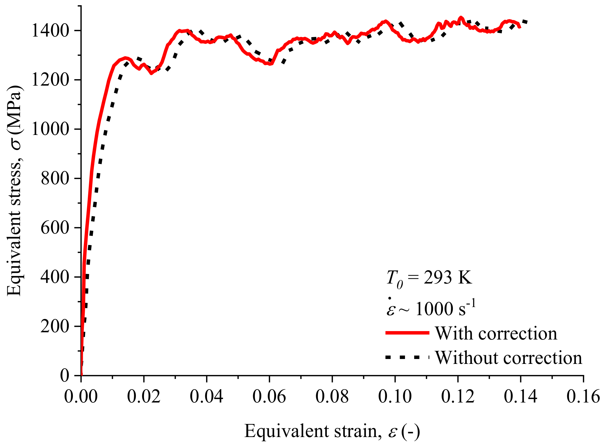
2.1.1. Experiments at Room Temperature

Uniaxial quasi-static experiments were performed using an electromechanical press. The use of the internal load cell sensor and an extensometer allowed to measure the values of the force F(t) and displacement δ(t) respectively. Experiments at strain rates ~500 and ~2000 s⁻¹ were done using a SHPB set-up. It is composed of a striker, an input and an output bar. All these parts have a diameter of 20.6 mm. The input and output bars are respectively 1900 mm and 1300 mm long, while the length of the striker is varying from 200–600 mm to change the loading time and the strain level induced into the specimen. From the gage measurement of the incident (${\epsilon }_i$), reflected (${\epsilon }_r$), and transmitted (${\epsilon }_t$) waves, the true stress and the true strain are calculated using the elastic waves propagation theory. The strain rate depending on time is defined as follows, Equation (1)

$$\dot{\epsilon }\left(t\right)=\frac{C_0}{l_0}\left({\epsilon }_i-{\epsilon }_r-{\epsilon }_t\right) \mathrm{where} C_0= \sqrt{\frac{E_{bar}}{{\rho }_{bar}}}$$

(1)

where $\dot{\epsilon }$ represents the nominal strain rate, $C_0$ the elastic wave velocity in the bars, and $E_{bar}$ and ${\rho }_{bar}$ the Young’s modulus and the density of the bars, respectively. The nominal strain, Equation (2) is obtained using the previous equation Equation (1) as

$$\epsilon \left(t\right)={{\displaystyle \int }}_0^t\dot{\epsilon }\left(\tau \right)d\tau$$

(2)

Moreover, for material such as high strength steel (HSS), punching effect can induce an overestimation of the strain level induced to the specimen. An analytic solution was developed by Safa and Gary [19] to take into account this effect, Figure 1. A comparison is reported using or not this correction. The variation of strain Δε is proportional to the stress level and therefore increases with strain for material with positive hardening. Thus, it is observed that the puncture effect is reduced to Δε^max ≈ 0.004 corresponding to ~2.6% for a strain level of ε^max = 0.15. For this reason, the correction is applied during the test analyses.

Concerning the true stress in dynamic compression, it is obtained using the transmitted wave ${\epsilon }_t$, Equation (3). This relation assumes the mechanical equilibrium during the test.

$$\sigma \left(t\right)=\frac{S_{\mathrm{bar}}}{S_0}{E}_{\mathrm{bar}}{\epsilon }_t\left(t\right)$$

(3)

where S_bar is the section of the bars and S₀ the section of the specimen. In general, the stress value is affected by the friction value μ between the bars and the specimen. Moreover, inertia may act on the stress in addition to friction. Due to these two effects, the stress level measured during the test must be corrected. Details of the related correction can be found in [16]. Highest strain rate experiments were performed using direct impact experiments [18,20]. The stress was obtained by the same procedure as the one used for SHPB and the strain was determined by optical measurement.

During dynamic experiments, a part of the plastic work is converted into heat and cannot be dissipated along the specimen, contrary to quasi-static loading. In the last case, the temperature is therefore assumed as constant and equal to the initial temperature imposed to the specimen. In dynamic conditions corresponding to adiabatic conditions, the temperature increases ΔT during the process of plastic deformation is defined in Equation (4) as

$$T\left(\epsilon \right)=T_0+\Delta T=T_0+\frac{\beta }{C_p{\rho }_s}{{\displaystyle \int }}_{{\epsilon }_e}^{{\epsilon }_p}\sigma d\epsilon$$

(4)

where $C_p$ is the specific heat at constant pressure, and ${\rho }_s$ is the specimen density. The parameter β is the Taylor–Quinney coefficient and corresponds to the part of the plastic work converted into heat and assumed for metals equal to 0.9. The values used in this work are reported in

Table 1. Material properties of the investigated high strength steel.

Es (GPa)	ρs (kg·m−3)	Cp (J·kg−1·K−1)	β (-)
210	7800	470	0.9

.

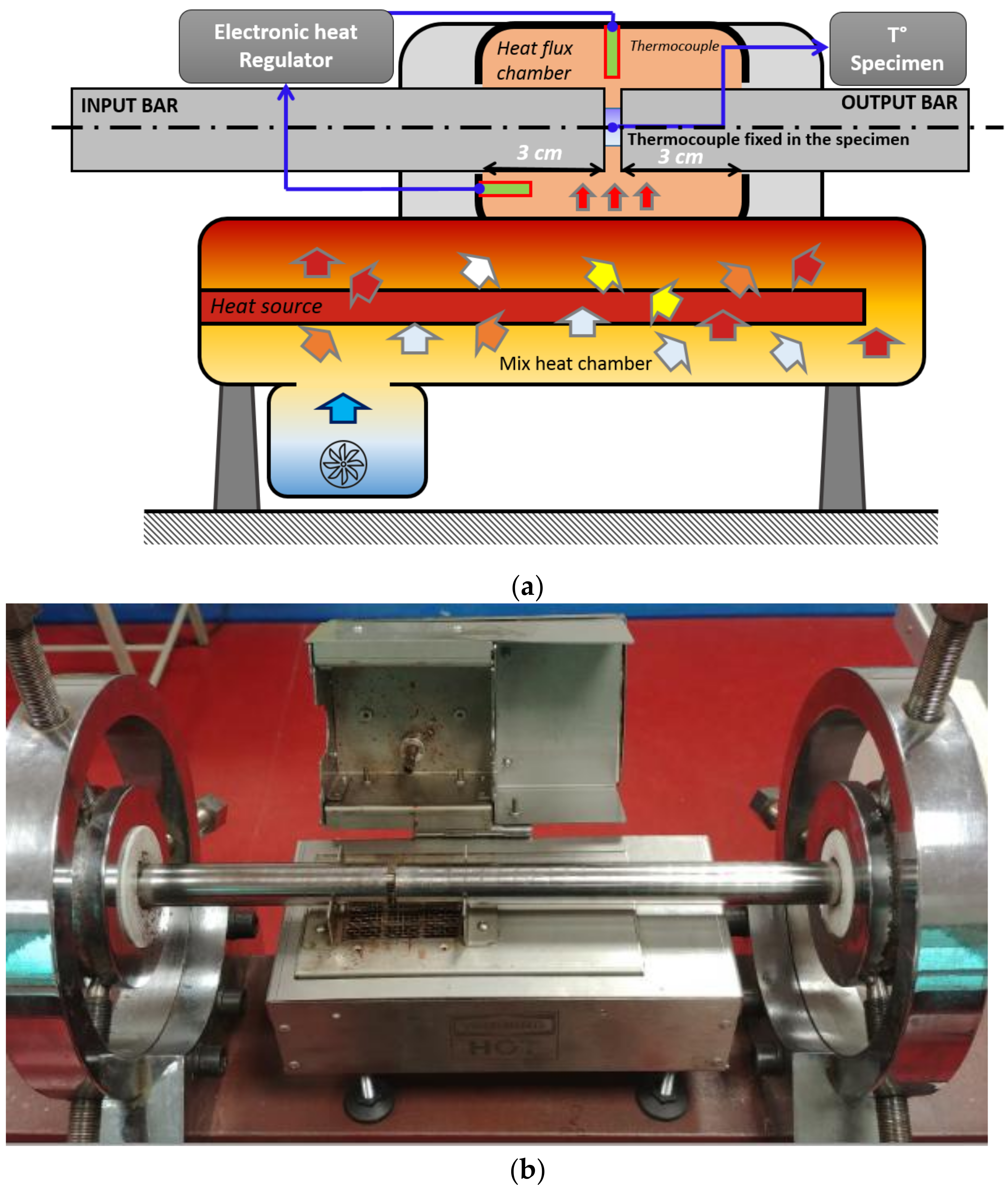
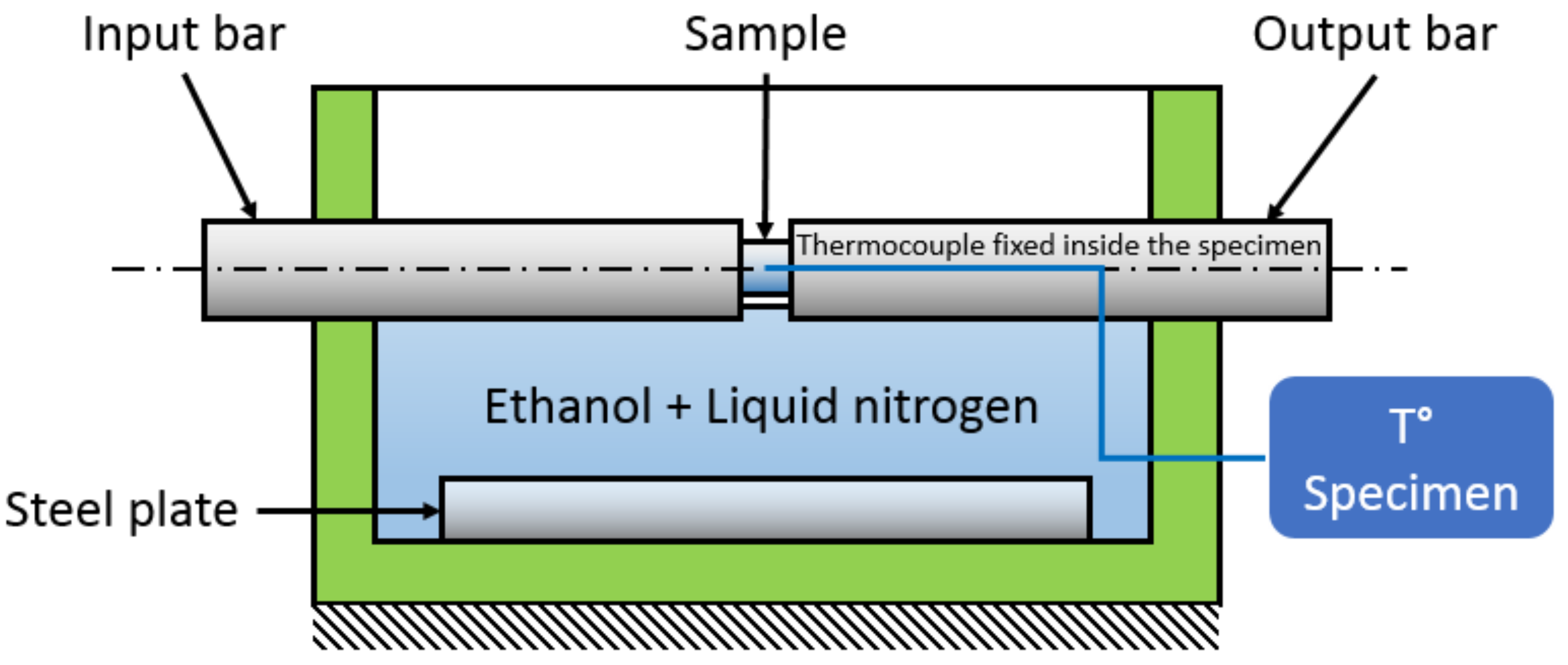
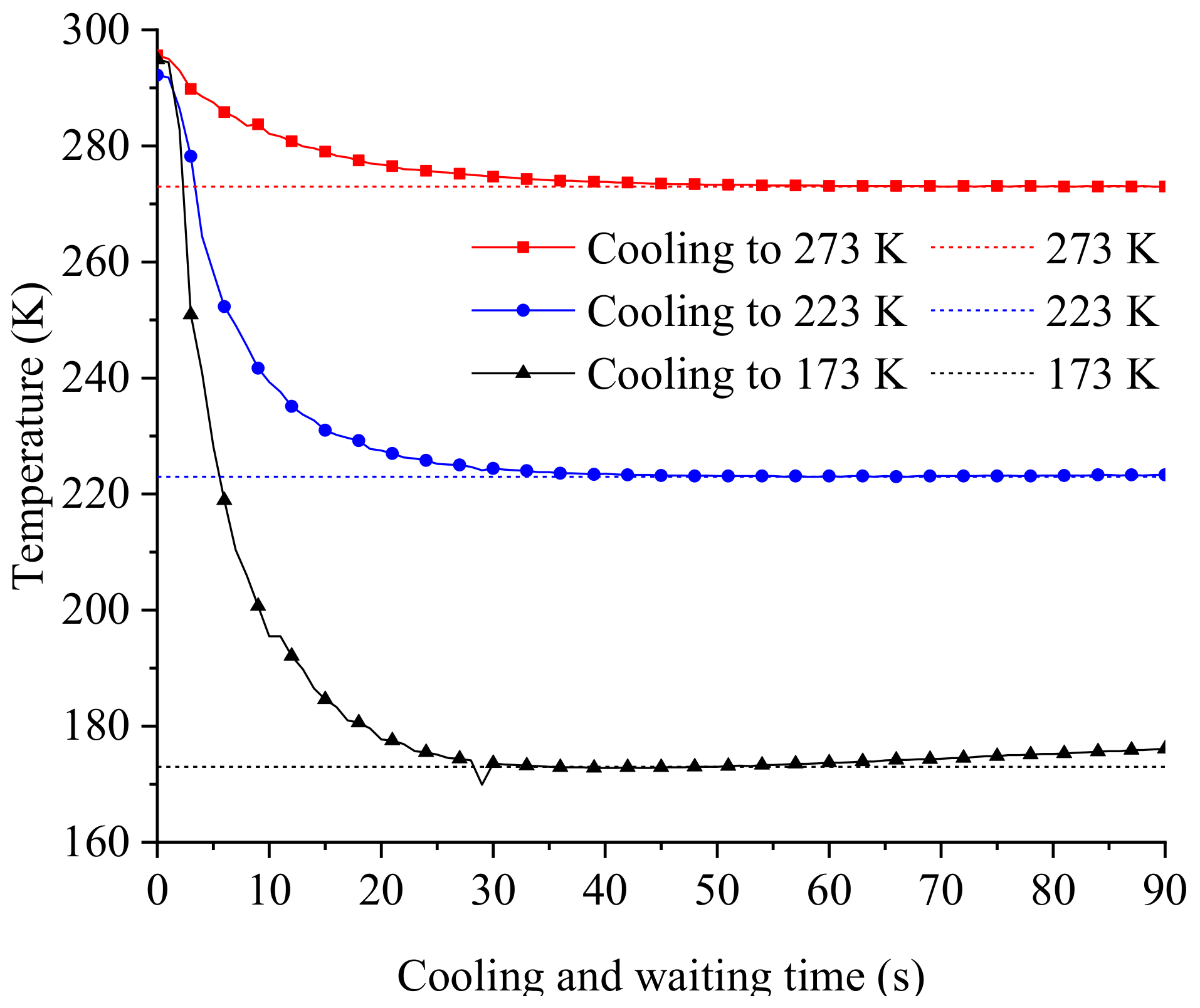
2.1.2. Experiments at Various Temperatures

In addition, and as discussed previously, thermal softening appears at high strain rates for deformations larger than 0.1. Therefore, an experimental study was carried out to determine the temperature sensitivity of the studied HSS material. Experiments at high temperatures for a strain rate equal to 0.001 s⁻¹ have been performed using a climatic chamber surrounding the sample and the compression platens. These platens were heated to an imposed temperature, and the specimen was then placed and heated during 30 min before the test. This procedure was used to avoid cooling the specimen by thermal conduction with the compression tools. The tests were performed with a constant strain rate controlled by an extensometer fixed on the compression platens. Each test was performed three times to ensure the repeatability of the experiments. High temperature experiments under dynamic conditions were carried out using a specific furnace heating the specimen and the bar ends. This furnace is similar to the one used by Rusinek et al. [21]. A description of this apparatus is given in Figure 2. If a hot specimen is placed in contact with the bars at room temperature, the thermal conduction induces a fast cooling of the specimen as described in [18]. To avoid this problem, the ends of the bars were heated in the furnace. All parts were heated for 30 min to reach a homogeneous temperature distribution within the specimen.

Experiments at low temperature were also carried out in the dynamic regime, using liquid nitrogen mixed with ethanol to adjust the temperature. Ethanol was chosen because of its melting temperature close to 159 K. The bars were in contact with the mixture to decrease their temperature, as described in Figure 3. This study assumes that the evolution of the elastic properties is negligible for these temperatures [22]. Moreover, no bending of the bars was observed during the test. The specimen was not in contact with the mixture, but was cooled by conduction. An instrumented specimen with a thermocouple was used to determine the temperature and the waiting time required before dynamic compression testing. The temperature was set by adding either liquid nitrogen or ethanol. Moreover, a thick steel plate was placed at the bottom of the cooling box to increase the thermal inertia of the mixture.

Once the temperature is stabilized, the instrumented specimen was removed and a sample was placed between the bars. The temperature recorded inside the instrumented specimen is shown in Figure 4. A stable temperature is reached by conduction after a cooling time between 30 and 40 s once the specimen is placed between the bars. Moreover, as the bars are cooled prior to the test, their thermal inertia allows one to maintain the temperature of the specimen for a duration long enough to perform the test. For example, for a target temperature of 173 K, the specimen is maintained between 172 K and 174 K for 35 s (from 30–65 s). For a target temperature of 273 K and 223 K, the temperature of the specimen is maintained (at ±1 K) for more than a minute.

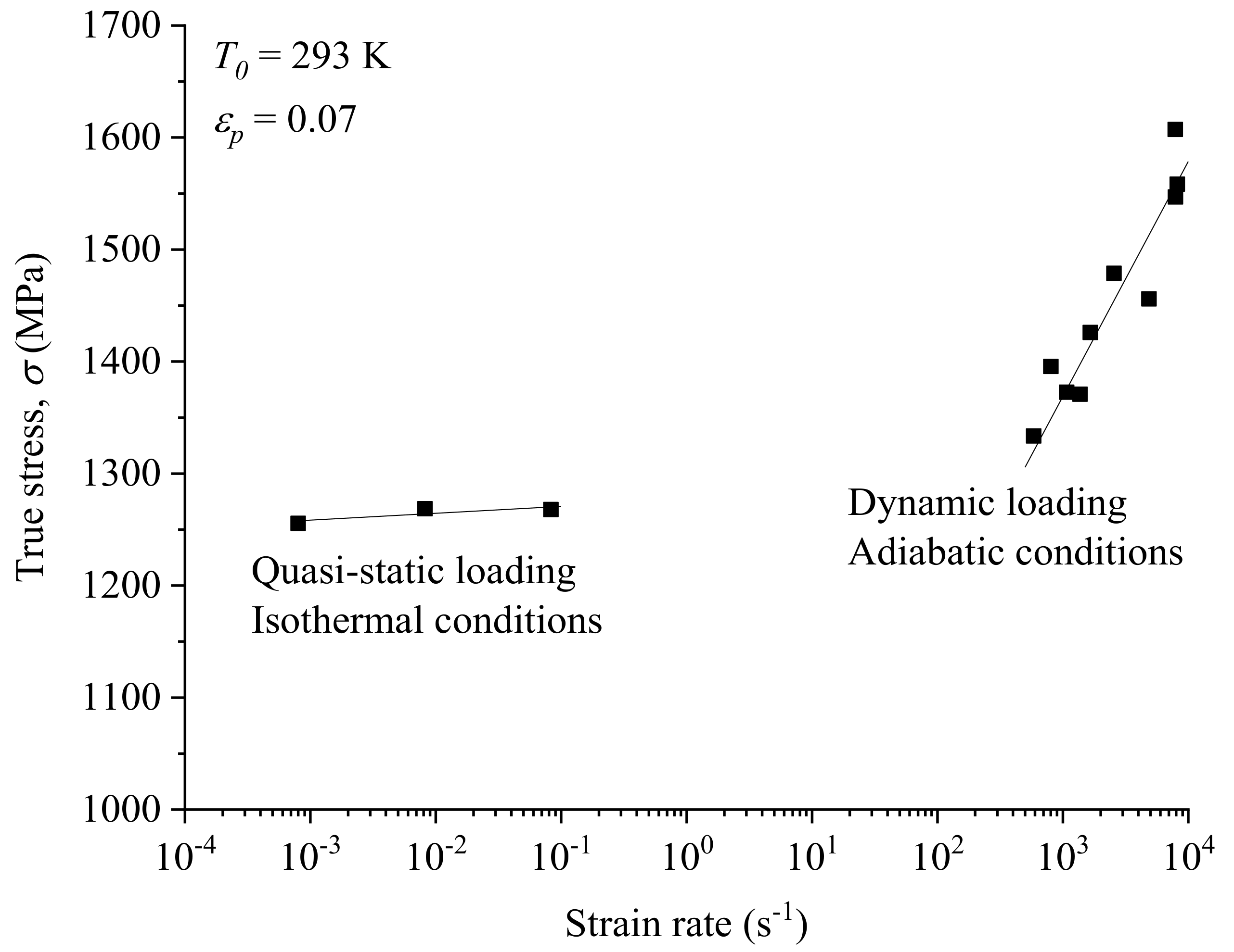
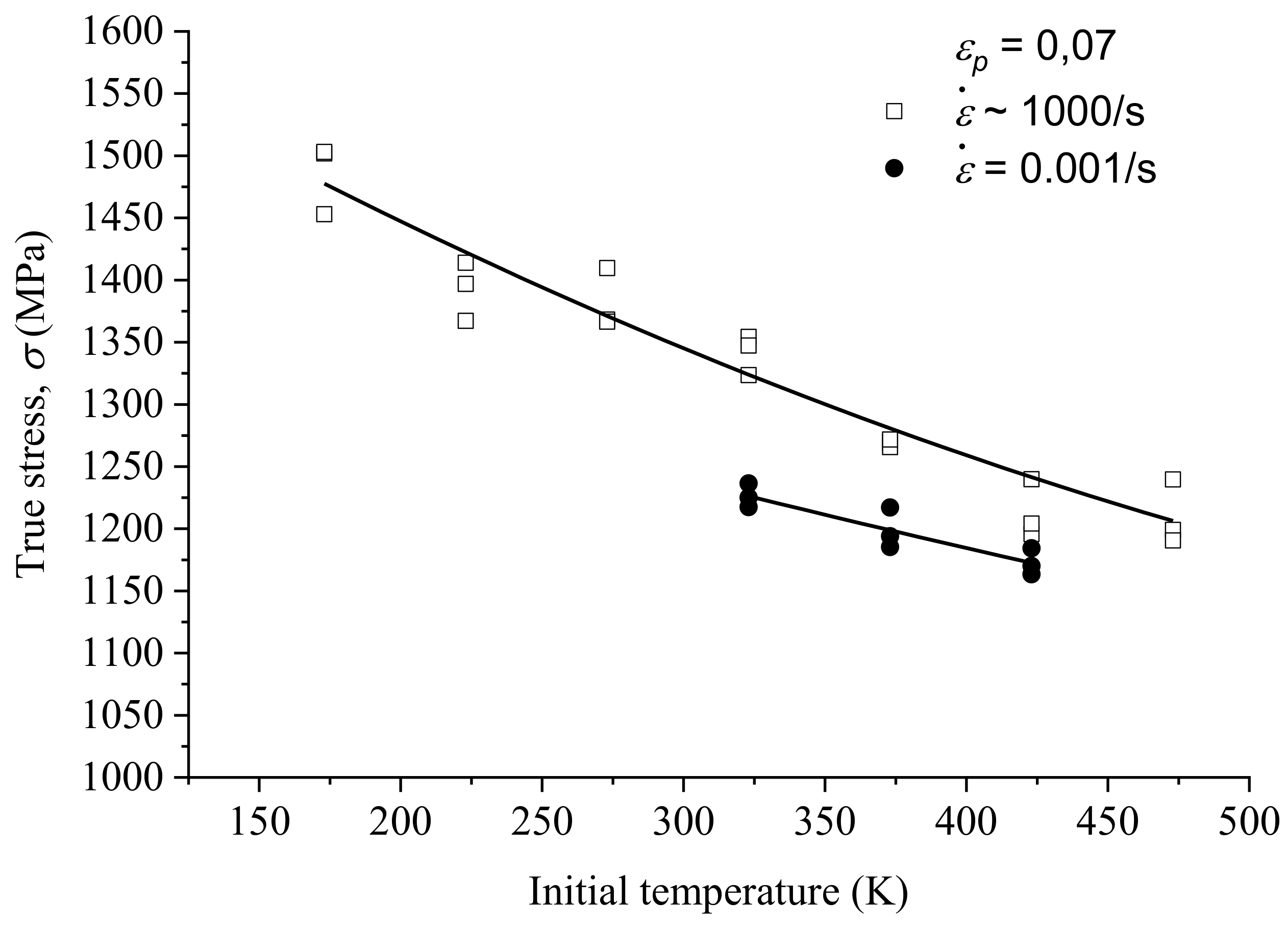
2.2. Experimental Results

The true stress values for each strain rate for a given strain level are represented in Figure 5. A plastic strain value below 0.1 was chosen to reduce the adiabatic heating effect on the stress. Therefore, the thermal softening effect is assumed to be negligible for this strain level. These experiments highlight a stress increase with the strain rate. Moreover, it has to be noticed that the strain rate sensitivity is much higher under dynamic conditions in comparison with low strain rates. The strain rate sensitivity, defined by $m=\partial \log \sigma /\partial \log \dot{\epsilon }$, is equal to 0.0021 for quasi-static loading and reaches 0.058 for dynamic loading. Thus, a nonlinear strain rate sensitivity is observed for the studied material and in general for metals [23,24,25].

The true stress values for each temperature and an imposed plastic strain level are reported in Figure 6. It has to be noted that the considered temperatures are corresponding to the initial temperatures (at the beginning of the test). The stress decreases as the temperature increases. The temperature sensitivity, defined by $\nu =\partial \log \sigma /\partial \log T$, is equal to −0.21 in dynamic loading conditions and decrease to −0.17 in quasi-static conditions.

Experiments have highlighted the effect of strain rate and temperature on the mechanical behavior of the studied HSS material.

2.3. Material Characterization of the Experimental Results

As discussed in the introduction, the theory of dislocation splitting the stress in two distinct parts is used to define the thermoviscoplastic behavior of materials. The equivalent stress for body cubic-centered (bcc) material is defined as τ = τ_μ + τ^* (with τ_μ corresponding to the athermal stress and τ^* the thermal stress), assuming an additive contribution of each part. Each component corresponds to a barrier preventing the dislocation motion. Two main categories are distinguished: long-range and short-range obstacles. The stress required to overcome the long-range barrier is represented by the athermal stress τ_μ and considers the obstacles such as grain boundaries or other dislocations. Therefore, this stress is related to the dislocation density into the considered material. For bcc metals, τ_μ is weakly affected by the strain rate or the temperature. The other component called the thermal stress τ^*, is representing the stress required to overcome the short-range obstacles. These obstacles correspond to the easiness for a dislocation to move from one site to the next, at an atomic level. At this scale, the motion of the dislocations requires to overcome the Peierls–Nabarro stress [23]. This stress corresponds to that required for the dislocation to move from one equilibrium position to the next. The energy required to overcome this barrier is temperature and strain rate dependent. On one hand, the temperature increase reduces the required energy by increasing the amplitude of atom vibrations which in turn facilitates the jump of individual atoms. On the other hand, higher strain rate induces a higher dislocation velocity and then a reduced time for the dislocations to move from one position to another. Therefore, the contribution of the thermal energy to overcome this barrier is weaker. These mechanisms are called thermally activated mechanisms. At T = 0 K, there is no contribution of the thermal energy, and the stress corresponding to the thermally activated mechanisms is maximum. This stress is called the mechanical threshold stress. This theoretical change of the equivalent flow stress with the temperature is represented in Figure 7 [26]. Below a critical temperature T_c, the flow stress corresponds to the addition of the thermal stress τ^* and the athermal stress, τ_μ. For temperature higher than T_c, the thermal stress vanishes and the flow stress is equal to the athermal stress.

Moreover, beyond a value of strain rate, dislocation motions become continuous. Their motion is then controlled by their interactions with phonons and electrons and corresponds to the phenomena of viscous drag. In these conditions, stress opposing to the dislocation motion is directly proportional to their velocity [27]. Nevertheless, the performed experiments did not reach strain rates high enough to observe such phenomenon.

The following section describes the constitutive relations studied in this work and the procedure used to define their constants based on previous experiments.

3. Constitutive Models

In this section, several models are compared with experiments to estimate their limits in term of strain rate and temperature. In this study, four models are analyzed. The first one is the well-known and widely used phenomenological Johnson–Cook model. The other models are defined as semi-physical since they are originally based on the dislocation theory discussed previously. The models described in this paper are the original versions proposed by Voyiadjis and Abed [15] and the Rusinek–Klepaczko models [1]. Moreover, two versions are proposed to update the model of Voyiadjis and Abed to describe in a more precise way the observed temperature and strain rate sensitivities.

3.1. Johnson–Cook Constitutive Model

The Johnson–Cook constitutive relation is a phenomenological model allowing one to describe the mechanical behavior of materials, Equation (5) [4]. It consists of splitting the different effects as the hardening, the temperature sensitivity, and the strain rate sensitivity in three multiplicative terms. Therefore, the first term represents the strain hardening, while the strain rate sensitivity and the thermal effect are introduced using respectively the second and third terms as shown below

$$\sigma \left({\epsilon }_p, {\dot{\epsilon }}_p,T\right)=\left(A+B{\epsilon }_p{}^n\right)\left[1+C\log \left(\frac{{\dot{\epsilon }}_p}{{\dot{\epsilon }}_0}\right)\right]\left(1-T^{*}{}^m\right)$$

(5)

where A, B, C, n and m are the model parameters and T^* is the homologous temperature. The parameters A, B and n represent respectively the yield stress, the modulus of plasticity and the hardening coefficient. The constant parameters are determined by fitting the true stress vs. true plastic strain curve for an assumed strain rate ${\dot{\epsilon }}_0$ and temperature T₀. The parameter C, representing the strain rate sensitivity, is determined by considering the stress level obtained for an imposed plastic strain level and different strain rates as shown in Figure 8a. The same procedure is applied to determine the parameter m, which represents the temperature sensitivity, as shown in Figure 8b.

The values of the parameters for the studied HSS material are reported in

Table 2. Parameters of the Johnson–Cook constitutive relation for the studied high strength steel.

A (MPa)	B (MPa)	n (-)	C (-)	m (-)	${\dot{\mathit{\epsilon }}}_0 \left(\mathit{s}{-}^1\right)$	T0 (K)	Tm (K)
1040.56	412.17	0.245	0.0122	0.98	0.0008	293	1785

. Considering this Johnson–Cook (JC) model, the parameters are easy to identify but its validity is limited. The term related to the strain rate assumes a linear sensitivity. This statement is valid for either the quasi-static or the dynamic observations, but does not fit the experimental data over the whole studied range. Moreover, a poor description of the strain rate sensitivity induces mistakes when instabilities are considered [28].

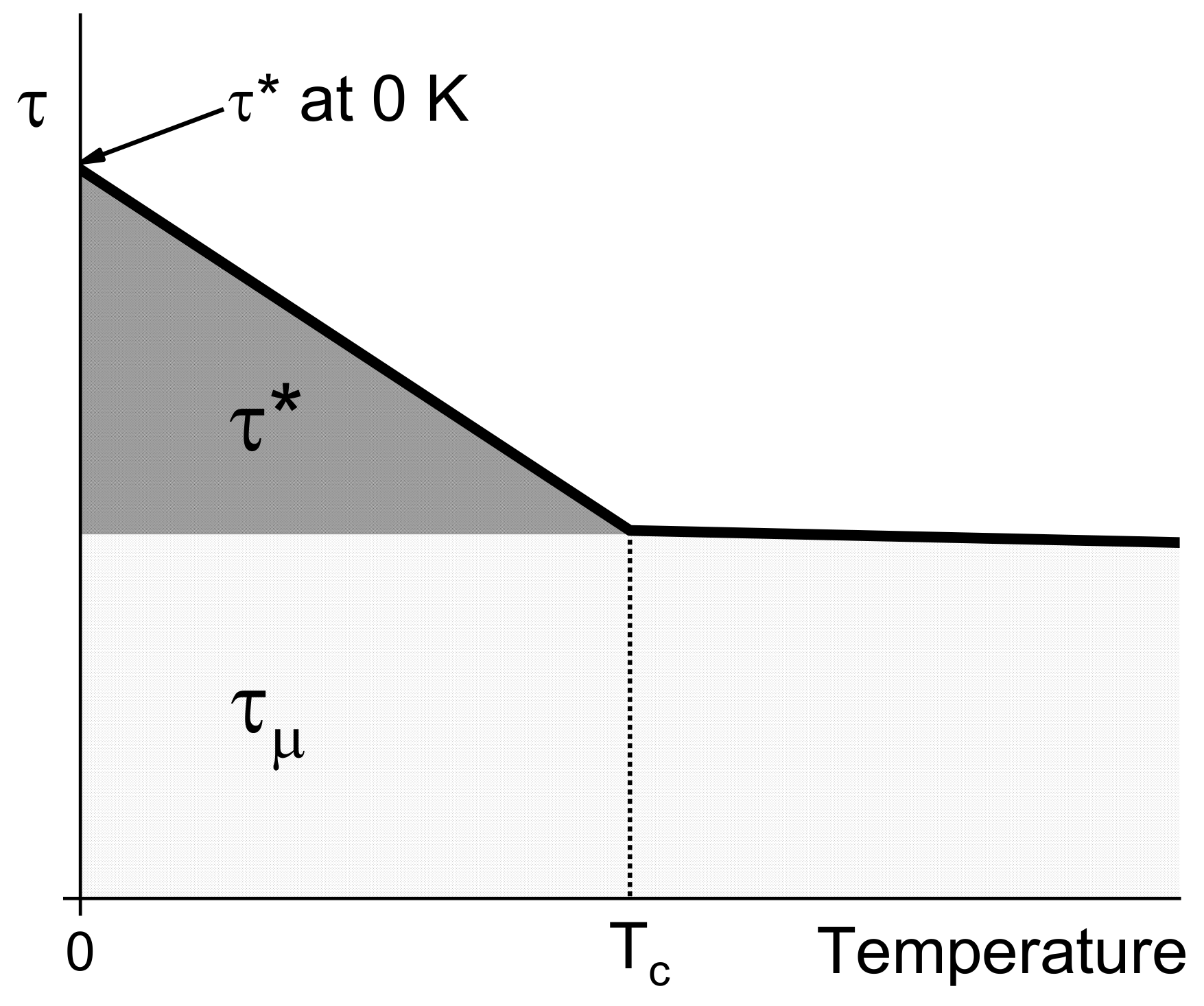
3.2. Voyiadjis–Abed Constitutive Model

The semi-physical model proposed by Voyiadjis and Abed [15] is based on the dislocations theory and the split of the equivalent stress into an athermal stress ${\sigma }_a$ and a thermal stress ${\sigma }_{th}$. The authors developed four specific constitutive relations, for body-centered cubic (bcc), face-centered cubic (fcc), hexagonal close-packed (hcp), and stainless steel microstructure. This study deals with the version developed for bcc metals. For most of these metals, the hardening is weakly influenced by the strain rate and the temperature [14]. Taking into account this consideration, the athermal stress is defined only as a function of the plastic strain. On the contrary, the thermal stress does not depend on the equivalent plastic strain, but depends on the strain rate and the temperature. Therefore, the constitutive relation is defined as follows, in Equation (6) as

$$\sigma \left({\epsilon }_p, {\dot{\epsilon }}_p,T\right)={\sigma }_a\left({\epsilon }_p\right)+{\sigma }_{th}\left({\dot{\epsilon }}_p,T\right)$$

(6)

where the previously discussed athermal stress ${\sigma }_a$, is defined using the first part of the Johnson–Cook constitutive model, Equation (7)

$${\sigma }_a\left({\epsilon }_p\right)=Y_a+B{\epsilon }_p{}^n$$

(7)

where $Y_a$ represents the yield stress, B is the modulus of plasticity, and n is the hardening coefficient. The thermal part ${\sigma }_{th}$ is defined by Equation (8). More details may be found in the work of Voyiadjis and Abed [15].

$${\sigma }_{th}\left( {\dot{\epsilon }}_p,T\right)=\tilde{\sigma }{\left(1-{\left({\beta }_{1}T-{\beta }_{2}T\ln \left({\dot{\epsilon }}_p\right)\right)}^{\frac{1}{q}}\right)}^{\frac{1}{p}}$$

(8)

where $\tilde{\sigma }$ represents the mechanical threshold stress, ${\beta }_1$ and ${\beta }_2$ are constants related to the dislocation density and $p$ and $q$ are constants related to the obstacles shape that dislocations have to overcome [29]. Thus, eight parameters have to be defined to model the behavior of the considered HSS material.

This constitutive relation assumes that the contribution of thermally activated mechanisms vanishes beyond a certain temperature. This assumption is used to identify the first three parameters $Y_a$, B, and n. As the stress observed for various temperatures do not evolve between 423 K and 473 K, it is assumed that for these temperatures, there is only a contribution of the athermal stress ${\sigma }_a$. Therefore, the results obtained at 473 K are used to identify $Y_a$, B, and n. The parameters $p$ and $q$ take the typical values as: p ∊ [0,1] and q ∊ [1,2]. In this work, 0.5 and 1.5 have been chosen for $p$ and $q$, respectively as proposed by [29]. The mechanical threshold stress $\tilde{\sigma }$, then corresponds to the value added to the athermal stress ${\sigma }_a$ in order to obtain the flow stress at 0 K. Consequently, for a fixed ${\dot{\epsilon }}_p$, the term ${\left(\sigma -Y_a-B{\epsilon }_p^n\right)}^p$ is plotted as a function of $T^{1/q}$ and approximated using a linear function, Figure 9. At T = 0 K, the following equality is reached ${\left(\sigma -Y_a-B{\epsilon }_p^n\right)}^p={\tilde{\sigma }}^p$, allowing to determine ${\tilde{\sigma }}^p$, as shown in Figure 9.

In order to determine ${\beta }_1$ and ${\beta }_2$, the term ${\left(1-{\left(\left(\sigma -Y_a-B{\epsilon }_p^n\right)/\tilde{\sigma }\right)}^p\right)}^q$ versus $\ln \left({\dot{\epsilon }}_p\right)$ is plotted for a fixed temperature. The results are reported in Figure 10a. The linear approximation is supposed to be equal to ${\beta }_1{T}_{room}-{\beta }_2{T}_{room}\ln \left({\dot{\epsilon }}_p\right)$ with T_room assumed as equal to 293 K. Nevertheless, the experimental data do not exhibit a linear behavior, especially under dynamic loading conditions. Therefore, all the domains defined in terms of strain rate may not be correctly modeled, as shown in Figure 10a. To obtain a better correlation with experimental observations a nonlinear approach is proposed, allowing one to model the non-linearity of the stress at high strain rates and to increase the strain rate sensitivity, as shown in Figure 10b. The thermal part, ${\sigma }_{th}$ is defined in this case using Equation (9) as

$${\sigma }_{th}\left( {\dot{\epsilon }}_p,T\right)=\tilde{\sigma }{\left(1-{\left({\beta }_{1}T-{\beta }_{2}T{\dot{\epsilon }}_p\right)}^{\frac{1}{q}}\right)}^{\frac{1}{p}}$$

(9)

The logarithm of the strain rate has been deleted as proposed in the modified JC model to avoid the stress linearity behavior with the strain rate [23,24,25].

However, using the second approach (Equation (9)) the quasi-static part is not well described. The solution to fit correctly the studied domain and to be in agreement with experiments is to combine the two previously detailed analytical relations Equations (8) and (9). This implies to define two domains corresponding to the quasi-static and dynamic regimes. Thus, the relation describing the strain rate sensitivity is composed of two parts. To ensure the continuity of the strain rate sensitivity definition between the two domains, it is necessary to impose the following conditions, Equations (10) and (11)

$${{\beta }_1^{Static}-{\beta }_2^{Static}\ln ({\dot{\epsilon }}_p^{Transition})={\beta }_1^{Dynamic}-{\beta }_2^{Dynamic}{\dot{\epsilon }}_p^{Transition}|}_{T_{room}}$$

(10)

$${\dot{\epsilon }}_p^{Transition}={\frac{{\beta }_2^{Static}}{{\beta }_2^{Dynamic}}|}_{T_{room}}\approx 403 {\mathrm{s}}^{-1}$$

(11)

The results are reported in Figure 11. Thus, the strain rate transition is defined by only the two coefficients ${\beta }_1$ and ${\beta }_2$. Using the HSS material, the transition strain rate to define the continuity of the strain rate sensitivity is equal to 403 s⁻¹.

Therefore, coupling Equation (8) and Equation (9), it is possible to fit experimental results performed at room temperature for a large range of strain rates with an improved accuracy. It has to be noted that a strain rate transition in order of 10² s⁻¹ is frequently observed for metals to describe the change between isothermal and adiabatic conditions. It induces a quick increase of the stress level with the strain rate [23,24,25]. Except for ${\beta }_1$ and ${\beta }_2$, these three versions of the constitutive relations developed by Voyiadjis and Abed have the same parameters, as reported in

Table 3. Common parameters of the three versions of Voyiadjis–Abed constitutive relations for the investigated high strength steel (HSS).

Ya (MPa)	B (MPa)	n (-)	$\tilde{\mathit{\sigma }}$ (MPa)	p (-)	q (-)
700	727.2	0.137	1018.39	0.5	1.5

.

The values for ${\beta }_1$ and ${\beta }_2$ for each approach are reported in

Table 4. Parameters ${\beta }_1$ and ${\beta }_2$ for each approach.

Approximation Used		β1	β2
Linear approach (original)		1.89 × 10−3	7.62 × 10−5
Nonlinear approach (modified)		2.07 × 10−3	1.56 × 10−7
Mixed approach	Linear part	2.04 × 10−3	4.02 × 10−5
	Nonlinear part	1.84 × 10−3	9.97 × 10−8

.

3.3. Rusinek–Klepaczko Constitutive Model

The Rusinek–Klepaczko semi-physical model reported in [1] is initially based on the theory of dislocations and the model proposed by Klepaczko [30]. This study deals with the original version reported in [1], although several authors [31,32,33] have proposed an extended version of this model. It decomposes the equivalent stress in an internal stress ${\sigma }_{\mu }$, related to long-range obstacles and an effective stress ${\sigma }^{*}$, related to short range obstacles, as in Equation (12)

$$\sigma \left({\epsilon }_p, {\dot{\epsilon }}_p,T\right)=\frac{E\left(T\right)}{E_0}\left[{\sigma }_{\mu }\left({\epsilon }_p, {\dot{\epsilon }}_p,T\right)+{\sigma }^{*}\left({\dot{\epsilon }}_p,T\right)\right]$$

(12)

where $E\left(T\right)$ and $E_0$ represent respectively the Young’s modulus depending on the temperature and at T = 0 K. Although this value can vary, the evolution of the Young’s modulus for steel [18] is assumed to be low enough (between 173 K and 473 K) in order to assume it as constant. The internal stress ${\sigma }_{\mu }$ is expressed by Equation (13)

$${\sigma }_{\mu }\left({\epsilon }_p, {\dot{\epsilon }}_p,T\right)=B\left({\dot{\epsilon }}_p,T\right){\left(\epsilon +{\epsilon }_0\right)}^{n\left({\dot{\epsilon }}_p,T\right)}$$

(13)

where ${\epsilon }_0$ is the strain level defining the yield stress, B and n are strain rate and temperature dependent coefficients and are defined as follows, in Equations (14) and (15)

$$B\left({\dot{\epsilon }}_p,T\right)=B_0{\left[\left(\frac{T}{T_m}\right)\log \left(\frac{{\dot{\epsilon }}_{max}}{{\dot{\epsilon }}_p}\right)\right]}^{-\nu }$$

(14)

$$n\left({\dot{\epsilon }}_p,T\right)=n_0\langle 1-D_2\left(\frac{T}{T_m}\right)\log \left(\frac{{\dot{\epsilon }}_p}{{\dot{\epsilon }}_{min }}\right)\rangle$$

(15)

Finally, the effective stress ${\sigma }^{*}$ is given by Equation (16)

$${\sigma }^{*}\left({\dot{\epsilon }}_p,T\right)={\sigma }_0^{*}\langle 1-D_1\left(\frac{T}{T_m}\right)\log {\left(\frac{{\dot{\epsilon }}_{max}}{{\dot{\epsilon }}_p}\right)\rangle }^{m^{*}}$$

(16)

where $B_0, \nu , n_0, D_2, {\sigma }_0^{*}, D_1$, and $m^{*}$ are the model parameters, ${\dot{\epsilon }}_{\max }$ and ${\dot{\epsilon }}_{\min }$ are the strain rate limits of the model and $T_m$ is the melting temperature. The Macaulay brackets are defined as: $x=x$ if x > 0 and $x=0$ otherwise. The internal stress ${\sigma }_{\mu }$ mimics the evolution of the dislocation density (creation and annihilation) which is affected by the strain (hardening), the strain rate and the temperature [34]. On the contrary, the effective stress ${\sigma }^{*}$ describes the coupling and the reciprocity between the strain rate and the temperature. From a physical point of view, it represents the difficulty of a dislocation to overcome an obstacle. This additional stress increases with the strain rate but tends to vanish as the temperature increases [35]. Therefore, the model neglects the effective stress at low strain rates at room and at high temperatures.

The first step consists in defining $D_1$, assuming that the effective stress ${\sigma }^{*}$ is equal to zero at low strain rate (10⁻³ s⁻¹ in the present case) and 293 K as suggested by Equation (17)

$$D_1={\left[\left(\frac{293}{T_m}\right)\log \left(\frac{{\dot{\epsilon }}_{max}}{0.001}\right)\right]}^{-1}$$

(17)

Assuming that the effective stress is equal to zero at low strain rate, it allows to determine a first approximation of B(0.001,293) and n(0.001,293). As the effective stress ${\sigma }^{*}$ corresponds to an instantaneous effect and the internal stress ${\sigma }_{\mu }$ to a history effect, the next step is to estimate the stress increase with strain rate for an imposed plastic strain level. Thus, Equation (18) allows one to determine the values of ${\sigma }_0^{*}$ and $m^{*}$.

$$\Delta {\sigma }_0^{*}\left({\dot{\epsilon }}_p,T\right)=\sigma \left({\epsilon }_p,{\dot{\epsilon }}_p,T\right)-\sigma \left({\epsilon }_p,0.001,293\right)$$

(18)

Once the effective stress ${\sigma }^{*}$ is defined, the values of $B\left({\dot{\epsilon }}_p,T\right)$ and $n\left({\dot{\epsilon }}_p,T\right)$ for different sets of conditions can be identified. Finally, Equation (14) and (15) are used to determine $B_0, \nu , n_0$, and $D_2$. Parameter values determined for this model are given in

Table 5. Parameters of the Rusinek–Klepaczko model for the investigated high strength steel.

${\mathit{D}}_1 (-)$	${\mathit{\sigma }}_0^{*} \left(\mathbf{MPa}\right)$	${\mathit{m}}^{*} (-)$	${\mathit{B}}_0 \left(\mathbf{MPa}\right)$	$\mathit{\nu } (-)$	${\mathit{n}}_0 (-)$	${\mathit{D}}_2 (-)$	${\mathit{\epsilon }}_0 (-)$	${\dot{\mathit{\epsilon }}}_{\mathit{m}\mathit{i}\mathit{n}} \left(\mathit{s}{-}^1\right)$	${\dot{\mathit{\epsilon }}}_{\mathit{m}\mathit{a}\mathit{x}} \left(\mathit{s}{-}^1\right)$	${\mathit{T}}_{\mathit{m}} \left(\mathbf{K}\right)$
0.33	1491.22	11.15	1473.2	0.0101	0.056	0	0.005	10−5	105	1785

.

4. Comparison of the Experiments with the Identified Constitutive Relations

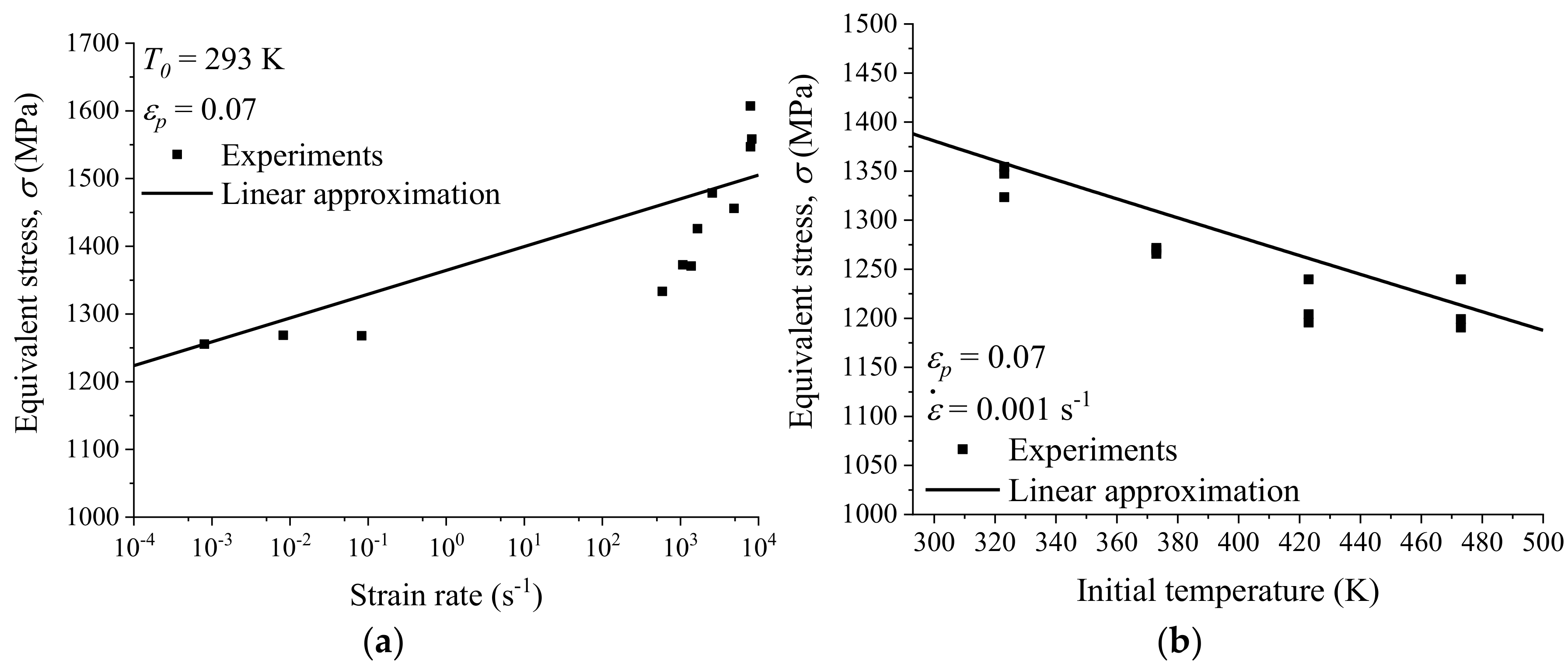
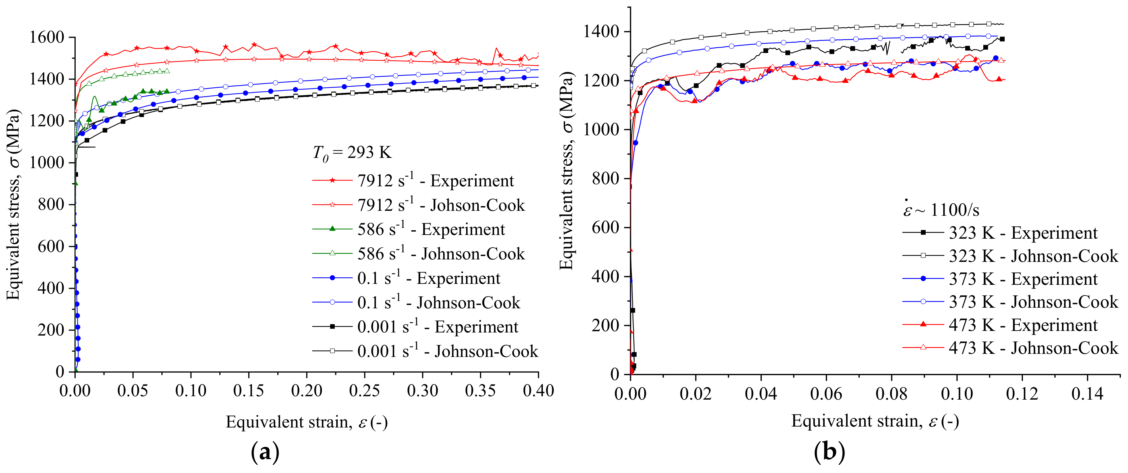
4.1. Comparison of the Experiments with the Johnson–Cook Model

A comparison between experiments and the Johnson–Cook model is shown in Figure 12a for different strain rates. As the strain rate varies during dynamic experiments, an average value has been calculated. It can be seen that hardening is well represented by the model in quasi-static loading, emphasizing that the first term of Equation (5) provides a good description of the material behavior in these conditions. Nevertheless, in the dynamic regime, one can observe that this constitutive relation does not fit the experimental data. It overestimates the stress at the lowest strain rates and underestimates at the highest. The Johnson–Cook model assumes a linear strain rate sensitivity of the stress, which is in contrast with experiments (Figure 8a). The comparison between the model and experiments is shown in Figure 12b for different temperatures. Experiments at various temperatures were performed at an average strain rate of about 1100 s⁻¹. This strain rate induces an overestimation of the flow stress due to the poor description of the strain rate sensitivity. Nevertheless, this model provides a correct description of the temperature sensitivity.

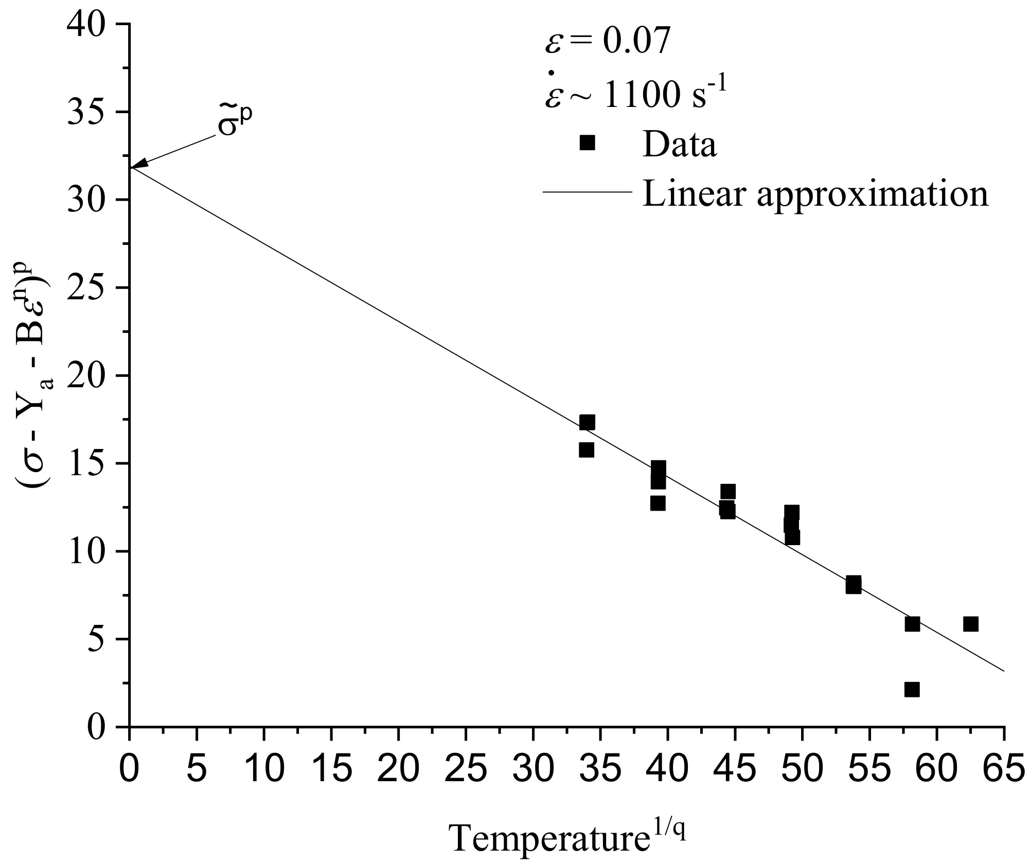
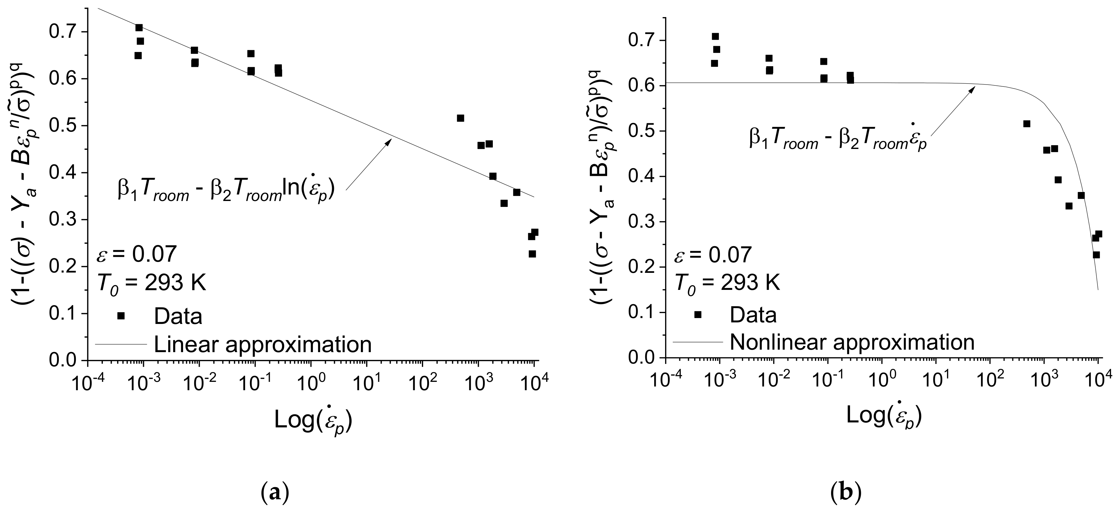
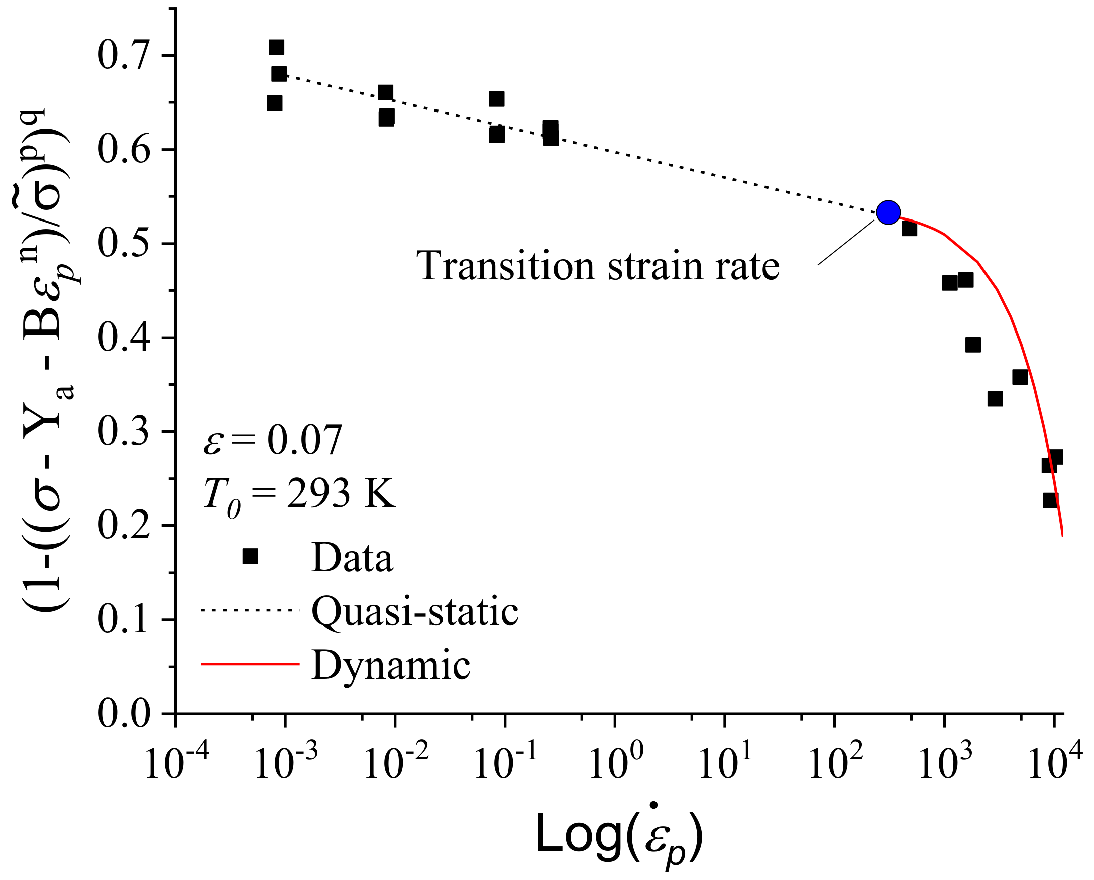
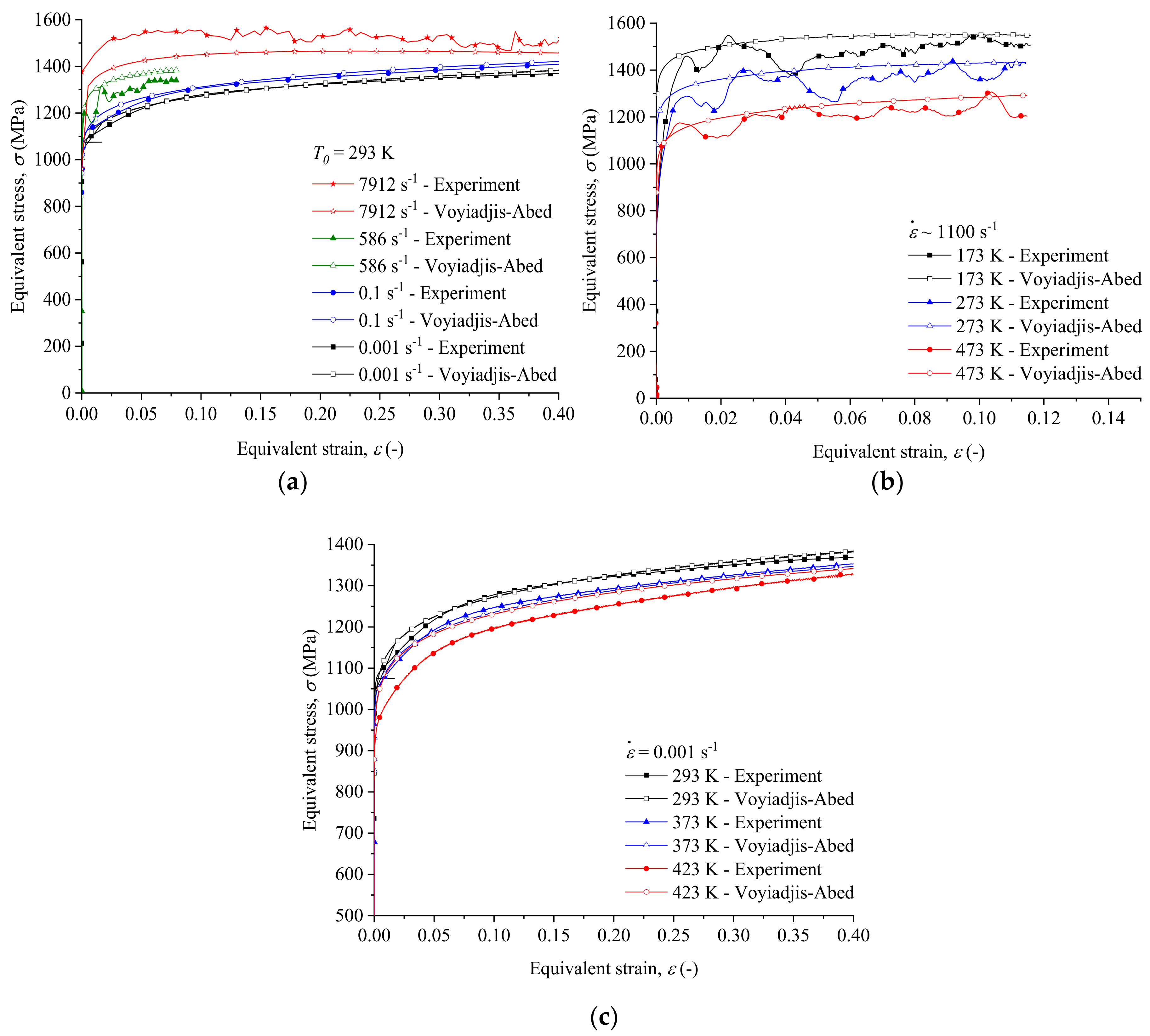
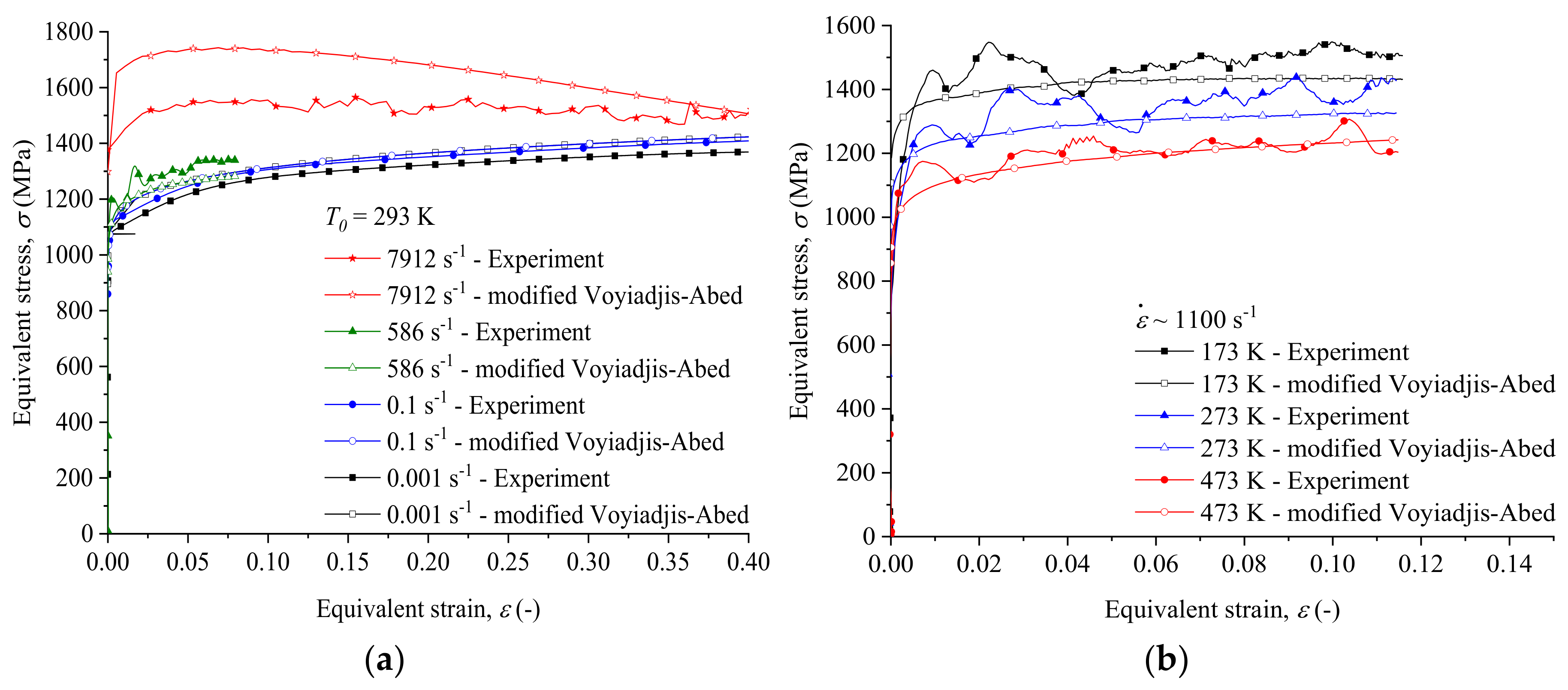
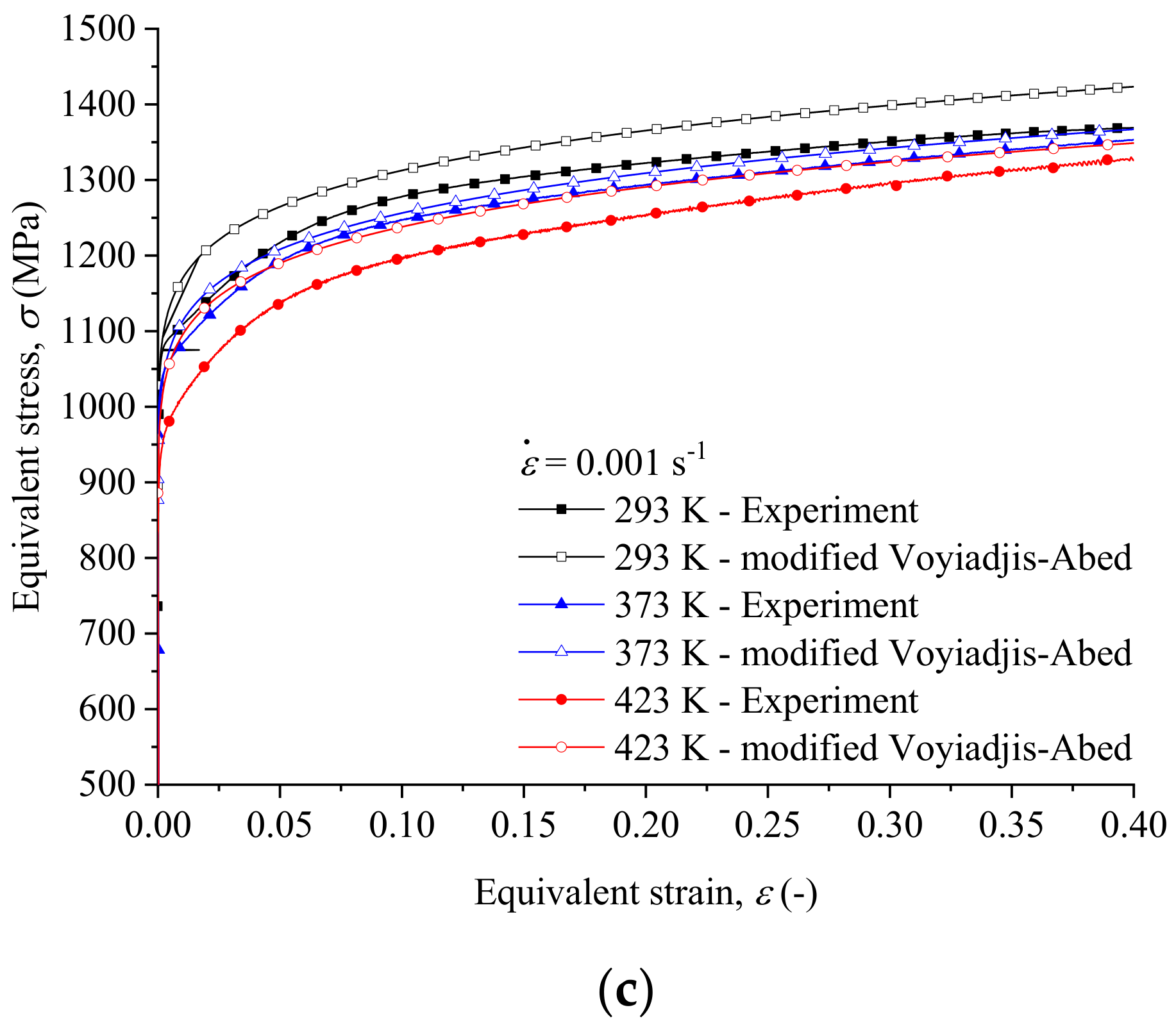
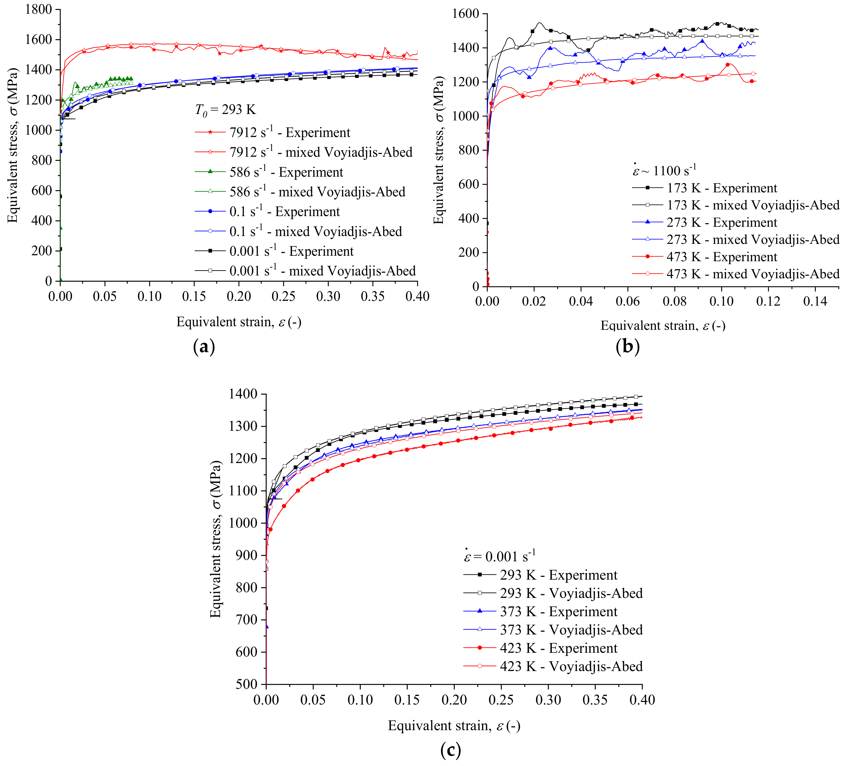
4.2. Comparison of Experiments with the Voyiadjis–Abed Model using Different Approaches

The comparison between constitutive relations and experiments are shown in Figure 13, Figure 14 and Figure 15 for the original linear, the modified non-linear and the mixed approaches. The strain rate sensitivity is not be well represented for a dynamic loading in the original version, Figure 13a. This is due to the linear sensitivity assumed by this model, as expressed in Equation (8). The flow stress value described by this model at 7912 s⁻¹ is ~50 MPa higher than the description at 586 s⁻¹, although experiments showed an increase of ~200 MPa. The non-linear modification brought to this model provides an overestimation of the strain rate sensitivity, as observed in Figure 14a. The flow stress at the highest reported strain rate (7912 s⁻¹) is overestimated. In dynamic conditions, the mixed approach uses the same equation of the thermal part of the flow stress, ${\sigma }_{th}$, defined by Equation (9). Therefore, the results obtained using the mixed approach are better than those obtained with previous versions, as shown in Figure 15a. The experimental values of the dynamic compression tests at various temperatures are well represented by these models, including at low temperature. The related comparisons are shown in Figure 13b, Figure 14b and Figure 15b. Regarding the temperature sensitivity at low strain rate, shown in Figure 13c, Figure 14c and Figure 15c, a correct description of the experiments is obtained at room temperature and for T₀ =373 K. However, the flow stress is overestimated at 423 K for all of the approaches.

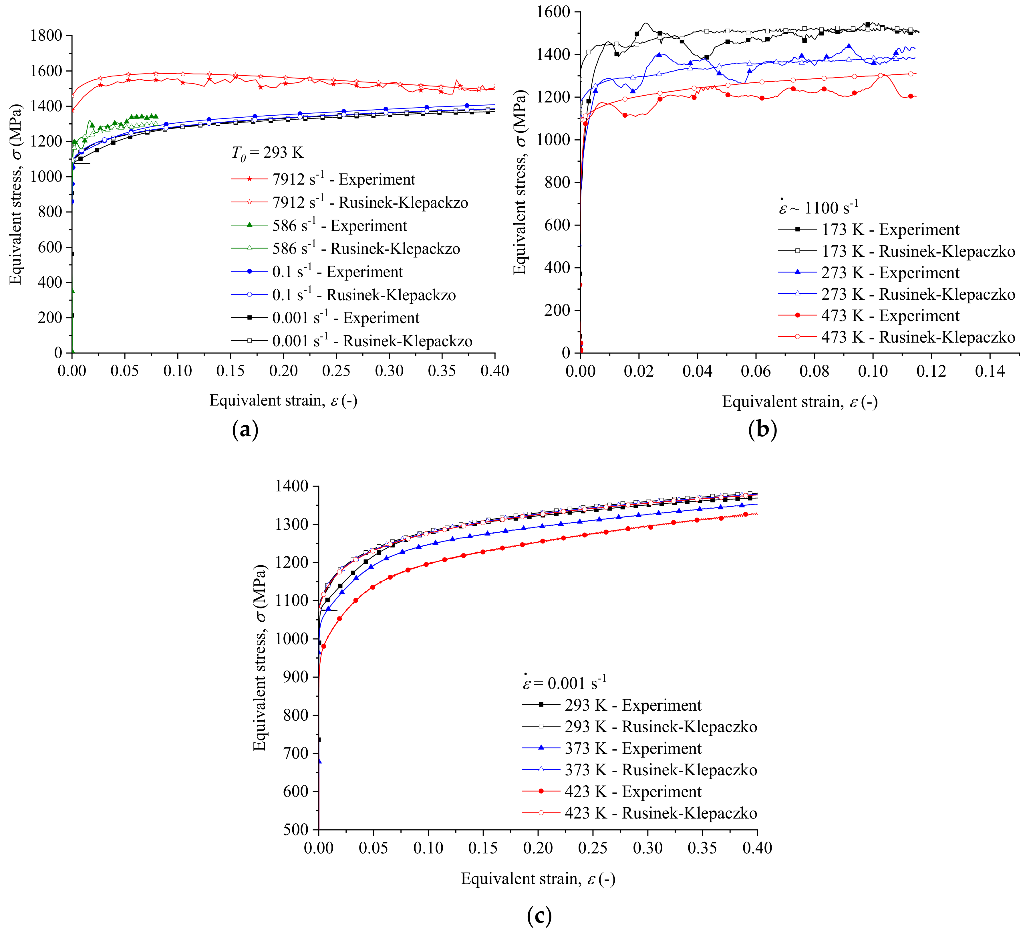
4.3. Comparison of Experiments with Rusinek–Klepaczko Model

A comparison, at different strain rates, between experiments and the model is shown in Figure 16a. The representation of the dynamic regime is similar to the one obtained with the modified Voyiadjis–Abed constitutive relation. Although the sensitivity in the quasi-static case is too low in comparison with experiment performed at 0.1 s⁻¹, this model is in good agreement with experimental measurements in most of the studied cases. Regarding experiments at various temperatures, this model provides a good description of the temperature sensitivity and the thermal softening (see Figure 16b). Figure 16c provides a comparison of the experimental results and the constitutive relation for the quasi-static compression tests at high temperature. The temperature sensitivity described by this model at 0.001 s⁻¹ is lower than the one observed experimentally.

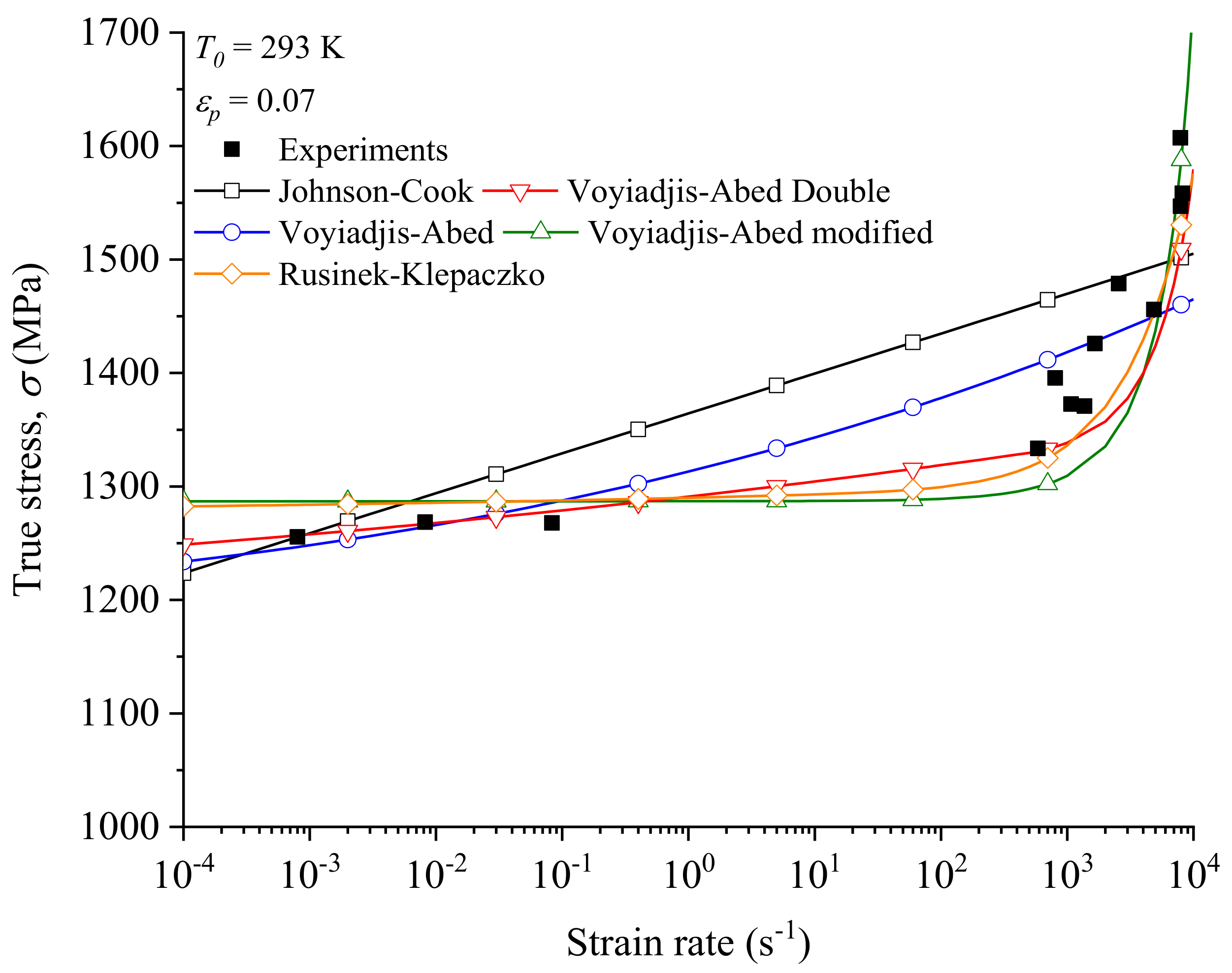
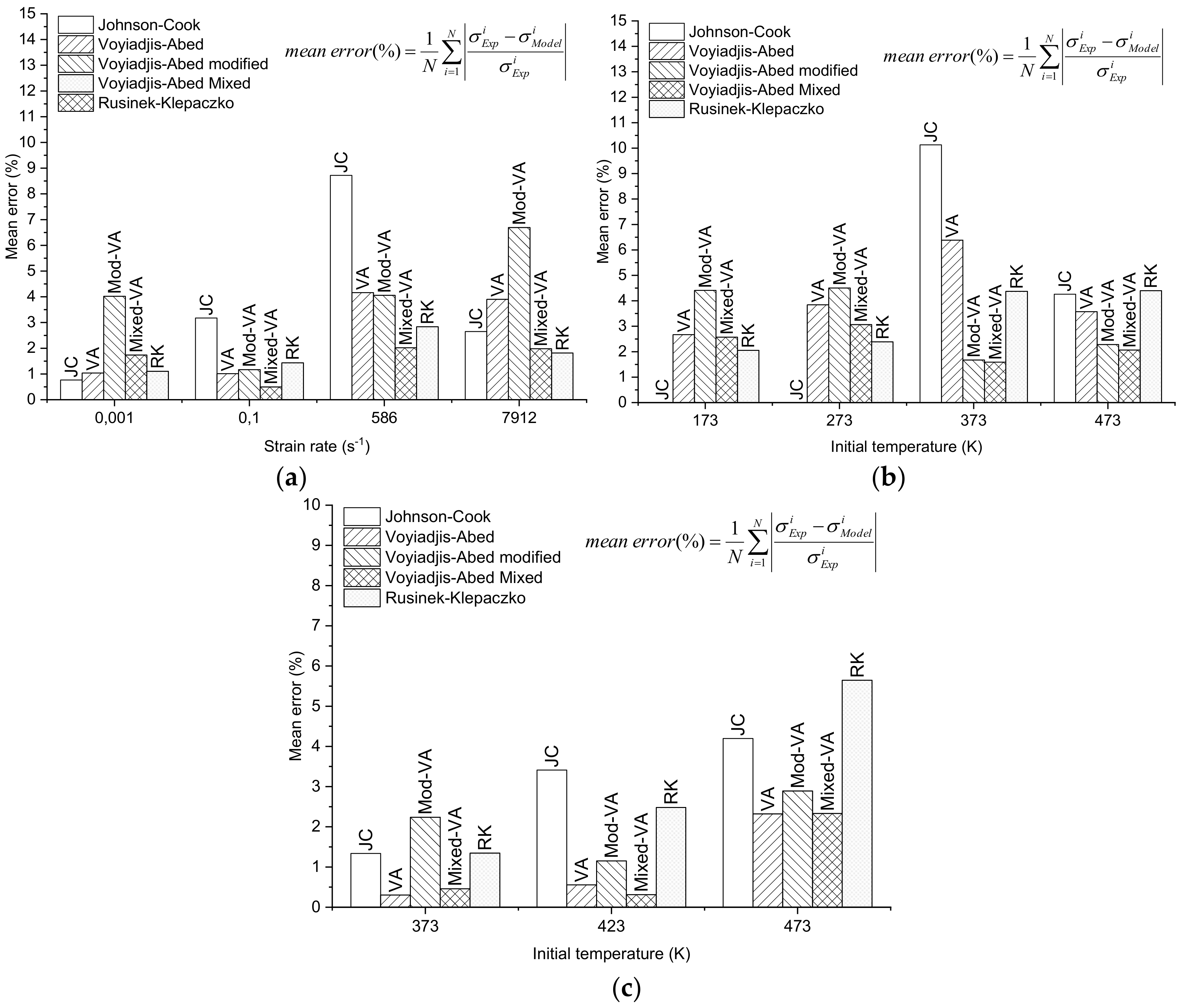
4.4. Comparison between Constitutive Relations and Limits

A comparison of the constitutive relations described previously is reported in Figure 17. It compares the macroscopic strain rate sensitivity described by the different models. It is observed that the Johnson–Cook model and the model defined originally by Voyiadjis and Abed do not allow to define the nonlinear strain rate sensitivity observed experimentally for metals as reported in [23,24,25]. To overcome this limitation, the model proposed by Rusinek and Klepaczko and the constitutive relation proposed by Voyiadjis and Abed (modified and using mixed approach) may be used. The three models are sensibly giving the same trends, Figure 17.

The modified Voyiadjis–Abed model presents a strain rate sensitivity at ${\epsilon }_p=0.07$ which is too low for low strain rates, and too high for high strain rates. The expression of the thermal part, ${\sigma }_{th}$ (Equation (9)) was chosen to represent the strong sensitivity observed for dynamic loadings. This explains the poor description obtained for quasi-static cases. Moreover, the parameters identification takes into account experiments at low strain rates and therefore increases the inaccuracies for dynamic loadings. The mixed approach used provides a compromise between the linear sensitivity observed at low strain rates and the nonlinear sensitivity at high strain rates. The Rusinek–Klepaczko constitutive relation provides a better representation of high strain rates experiments, but underestimates the sensitivity for quasi-static cases. It has to be noted that the values of Figure 17 represent the flow stress for fixed strain level. In order to compare the efficiency of the models, the mean error expressed in Equation (19) was calculated for several cases for each constitutive relation.

$$Mean error (\%)=\frac{1}{N}{\displaystyle \sum }_{i=1}^N\left(\frac{{\sigma }_{exp}^i-{\sigma }_{model}^i}{{\sigma }_{exp}^i}\right)\times 100$$

(19)

The comparison of errors obtained for various strain rates at room temperature for each constitutive relation is shown in Figure 18a. For a strain rate value of $\dot{\epsilon }$= 0.001 s⁻¹, the Johnson–Cook constitutive relation provides a better description than the others models. This is explained by the fact that this loading conditions (0.001 s⁻¹, 293 K) was taken as a reference to identify the parameters of this model. The errors obtained are globally higher for high strain rates. The mixed approach of the Voyiadjis–Abed model and the Rusinek–Klepaczko constitutive relation present best agreement for dynamic cases. The error comparisons obtained for various temperatures at ~1100 s⁻¹ for each constitutive relation is shown in Figure 18b. Regarding the Johnson–Cook model, no comparison can be established between this model and experiments below the reference temperature used during the parameters identification (293 K). Other models provide a good description of the temperature sensitivity for dynamic loading. The gaps obtained for various temperatures at 0.001 s⁻¹ for each constitutive relation is shown in Figure 18c. As shown in Figure 6, the thermal sensitivity of this material is strain rate dependent. The Johnson–Cook model assumes a constant thermal sensitivity regardless of the strain rate. Moreover, the Rusinek–Klepaczko underestimates this sensitivity at 0.001 s⁻¹. This explains higher errors observed in quasi-static conditions compared to the other constitutive relations. The other models provide good description of the temperature sensitivity for quasi-static loading. For every model, the highest error is observed at the highest studied temperature, in quasi-static conditions. As a consequence, when studying the case of impact loading, the best compromise can be found with the mixed approach of the Voyiadjis–Abed constitutive relation due to its ability to describe high strain rate phenomena without degrading low strain rate representation.

5. Conclusions

The mechanical behavior of a high strength steel was studied, with experiments performed over a wide range of strain rates varying from 10⁻³–10⁴ s⁻¹ and various temperatures starting from 173 K to 473 K. This experimental investigation allowed to highlight the different sensitivities of this high strength steel. The parameters of five different constitutive relations were identified and the results were compared to the experiments. The first one is the Johnson–Cook constitutive model. This model provides a good description of the temperature sensitivity, but only for temperatures above the reference temperature (293 K in this work). Furthermore, it assumes a linear strain rate sensitivity, which is not the case of the studied material, and cannot represent any coupling effect between the strain rate and the temperature. Nevertheless, among the considered relation, its parameters are the easiest to determine and it allows a correct description of the material mechanical behavior at conditions close to those chosen as references. In order to overcome these limitations, two semi-physical models are considered. The constitutive relation developed by Voyiadjis and Abed gives a better description of the thermal sensitivities over a wide range of strain rates. Nevertheless, the strain rate sensitivity is not well fitted, especially at high strain rates. A modified nonlinear version for dynamic cases has been suggested. Nevertheless, this modification degrades the representation of low strain rates. Therefore, a mixed approach using a transition between low and high strain rates has been suggested. This model provides a better description at high strain rates and is more consistent with the observed trend. Moreover, it offers a good correlation with tests at various temperatures. The last studied model has been developed by Rusinek and Klepaczko. This constitutive relation allows description of the sensitivities observed experimentally but presents higher mean errors than the mixed approach of the Voyiadjis and Abed model for temperature sensitivity description. It should be noted that the modified and the mixed versions of the Voyiadjis–Abed model have a maximal strain rate limit at ~10⁴ s⁻¹. From a physical point of view, other phenomena, such as viscous drag, become preponderant beyond this value and are not taken into account in these models. Regarding the Rusinek–Klepaczko model, an extension has been studied in [33] to introduce this effect.

References

1. Rusinek, A.; Klepaczko, J.R. Shear testing of a sheet steel at wide range of strain rates and a constitutive relation with strain-rate and temperature dependence of the flow stress. Int. J. Plast. 2001, 17, 87–115. [Google Scholar] [CrossRef]
2. Nemat-Nasser, S.; Guo, W.G. Thermomechanical response of DH-36 structural steel over a wide range of strain rates and temperatures. Mech. Mater. 2003, 35, 1023–1047. [Google Scholar] [CrossRef]
3. Rusinek, A.; Rodríguez-Martínez, J.A.; Klepaczko, J.R.; Pecherski, R.B. Analysis of thermo-visco-plastic behaviour of six high strength steels. Mater. Des. 2009, 30, 1748–1761. [Google Scholar] [CrossRef]
4. Johnson, G.R.; Cook, W.H. A constitutive model and data for metals subjected to large strain, high strain rates and high temperatures. In Proceedings of the 7th International Symposium on Ballistics, Hague, The Netherlands, 19–21 April 1983. [Google Scholar]
5. Johnson, G.R. Implementation of simplified constitutive models in large computer codes. In Dynamic Constitutive/Failure Models; Rajendran, A.M., Nicholas, T., Eds.; University of Dayton report: Dayton, OH, USA, 1988; pp. 409–418. [Google Scholar]
6. Mecking, H.; Kocks, U.F. Kinetics of flow and strain-hardening. Acta Met. 1981, 29, 1865–1875. [Google Scholar] [CrossRef]
7. Follansbee, P.S.; Kocks, U.F. A constitutive description of the deformation of copper based on the use of the mechanical threshold stress as an internal state variable. Acta Met. 1988, 36, 81–93. [Google Scholar] [CrossRef] [Green Version]
8. Bammann, D.J. Modeling Temperature and Strain Rate Dependent Large Deformations of Metals. Appl. Mech. Rev. 1990, 43, S312. [Google Scholar] [CrossRef]
9. Bammann, D.J.; Johnson, G.C.; Chiesa, M.L. A Strain Rate Dependent Flow Surface Model of Plasticity; SAND90-8227; Sandia National Laboratory Report: Livermore, CA, USA, 1990.
10. Milella, P.P. On the Dependence of the Yield Strength of Metals on Temperature and Strain Rate. The Mechanical Equation of the Solid State. AIP Conf. Proc. 2002, 620, 642–648. [Google Scholar] [CrossRef]
11. Rodríguez-martínez, J.A.; Rusinek, A.; Pesci, R.; Zaera, R. Experimental and numerical analysis of the martensitic transformation in AISI 304 steel sheets subjected to perforation by conical and hemispherical projectiles. Int. J. Solids Struct. 2013, 50, 339–351. [Google Scholar] [CrossRef] [Green Version]
12. Rodríguez-martínez, J.A.; Pesci, R.; Rusinek, A.; Arias, A.; Zaera, R.; Pedroche, D.A. Thermo-mechanical behaviour of TRIP 1000 steel sheets subjected to low velocity perforation by conical projectiles at different temperatures. Int. J. Solids Struct. 2010, 47, 1268–1284. [Google Scholar] [CrossRef] [Green Version]
13. Hoge, K.G.; Mukherjee, A.K. The temperature and strain rate dependence of the flow stress of tantalum. J. Mater. Sci. 1977, 12, 1666–1672. [Google Scholar] [CrossRef]
14. Zerilli, F.J.; Armstrong, R.W. Dislocation-mechanics-based constitutive relations for material dynamics calculations. J. Appl. Phys. 1987, 61, 1816–1825. [Google Scholar] [CrossRef] [Green Version]
15. Voyiadjis, G.Z.; Abed, F.H. Microstructural based models for bcc and fcc metals with temperature and strain rate dependency. Mech. Mater. 2005, 37, 355–378. [Google Scholar] [CrossRef]
16. Malinowski, J.Z.; Klepaczko, J.R. A Unified Analytic and Numerical Approach to Specimen Behaviour in the Split-Hopkinson Pressure bar. Int. J. Mech. Sci. 1986, 28, 381–391. [Google Scholar] [CrossRef]
17. Davies, E.D.; Hunter, S.C. The Dynamic Compressios Testing of Solids by the Method of the Split Hopkinson Pressure Bar. J. Mech. Phys. Solids 1963, 11, 155–179. [Google Scholar] [CrossRef]
18. Ramesh, K.T. High rates and impact experiments. In Handbook of Experimental Solid Mechanics; Sharpe, W.N., Jr., Ed.; Springer: Boston, MA, USA, 2008; pp. 929–959. [Google Scholar]
19. Safa, K.; Gary, G. Displacement correction for punching at a dynamically loaded bar end. Int. J. Impact Eng. 2010, 37, 371–384. [Google Scholar] [CrossRef] [Green Version]
20. Malinowski, J.Z.; Klepaczko, J.R.; Kowalewski, Z.L. Miniaturized compression test at very high strain rates by direct impact. Exp. Mech. 2007, 47, 451–463. [Google Scholar] [CrossRef]
21. Rusinek, A.; Bernier, R.; Boumbimba, R.M.; Klosak, M.; Jankowiak, T.; Voyiadjis, G.Z. New devices to capture the temperature effect under dynamic compression and impact perforation of polymers, application to PMMA. Polym. Test. 2018, 65, 1–9. [Google Scholar] [CrossRef]
22. Ledbetter, H.M.; Weston, W.F.; Naimon, E.R. Low-temperature elastic properties of four austenitic stainless steels. J. Appl. Phys. 1975, 46, 3855–3860. [Google Scholar] [CrossRef]
23. Meyers, M. Dynamic Behavior of Materials; John Wiley & Sons, Inc.: Hoboken, NJ, USA, 1994; ISBN 047158262X. [Google Scholar]
24. Regazzoni, G.; Kocks, U.F.; Follansbee, P.S. Dislocation kinetics at high strain rates. Acta Metall. 1987, 35, 2865–2875. [Google Scholar] [CrossRef]
25. Schulze, V.; Vöhringer, O.; Halle, T. Plastic Deformation: Constitutive Description. Mater. Sci. Mater. Eng. 2017. [Google Scholar] [CrossRef]
26. Hull, D.; Bacon, D.J. Introduction to Dislocations; Elsevier Ltd.: New York, NY, USA, 2011. [Google Scholar]
27. Granato, A.V. Microscopic Mechanisms of Dislocation Drag. In Proceedings of the Metallurgical Effects at High Strain Rates, Albuquerque, NM, USA, February 5–8 1973; Rohde, R.W., Butcher, B.M., Holland, J.R., Karnes, C.H., Eds.; Plenum Press: New York, NY, USA, 1973. [Google Scholar]
28. Hart, E.W. Theory of the tensile test. Acta Metall. 1967, 15, 351–355. [Google Scholar] [CrossRef]
29. Kocks, U.F. Realistic constitutive relations for metal plasticity. Mater. Sci. Eng. A 2001, 317, 181–187. [Google Scholar] [CrossRef]
30. Klepaczko, J.R. Physical-state variables-Key to constitutive modeling in dynamic plasticity. Nucl. Eng. Des. 1991, 127, 103–115. [Google Scholar] [CrossRef]
31. Rodríguez-martínez, J.A.; Rusinek, A.; Klepaczko, J.R. Constitutive relation for steels approximating quasi-static and intermediate strain rates at large deformations. Mech. Res. Commun. 2009, 36, 419–427. [Google Scholar] [CrossRef]
32. Rodríguez-martínez, J.A.; Rodríguez-millán, M.; Rusinek, A.; Arias, A. A dislocation-based constitutive description for modeling the behavior of FCC metals within wide ranges of strain rate and temperature. Mech. Mater. 2011, 43, 901–912. [Google Scholar] [CrossRef] [Green Version]
33. Rusinek, A.; Rodríguez-Martínez, J.A. Thermo-viscoplastic constitutive relation for aluminium alloys, modeling of negative strain rate sensitivity and viscous drag effects. Mater. Des. 2009, 30, 4377–4390. [Google Scholar] [CrossRef]
34. Klepaczko, J. Thermally activated flow and strain rate history effects for some polycrystalline fcc metals. Mater. Sci. Eng. 1975, 18, 121–135. [Google Scholar] [CrossRef]
35. Klepaczko, J.R.; Rusinek, A.; Rodríguez-Martínez, J.A.; Pecherski, R.B.; Arias, A. Modelling of thermo-viscoplastic behaviour of DH-36 and Weldox 460-E structural steels at wide ranges of strain rates and temperatures, comparison of constitutive relations for impact problems. Mech. Mater. 2009, 41, 599–621. [Google Scholar] [CrossRef] [Green Version]
Figure 1. Comparison of the results obtained with and without the punching correction in dynamic compression.
Metals 08 00795 g001
Figure 2. Description (adapted from [21]) (a) and picture (b) of the furnace used for high temperature dynamic compression tests.
Metals 08 00795 g002
Figure 3. Description of the technique used to perform dynamic compression at low temperature.
Metals 08 00795 g003
Figure 4. Evolution of the temperature inside a specimen placed between the cold bars.
Metals 08 00795 g004
Figure 5. True stress vs. strain rate for a strain level of ε p = 0.07 ε p = 0.07 at room temperature during compression tests.
Metals 08 00795 g005
Figure 6. True stress vs. initial temperature, in quasi-static and dynamic conditions, under compression.
Metals 08 00795 g006
Figure 7. Temperature effect on the flow stress decomposed using additive description.
Metals 08 00795 g007
Figure 8. Identification of the parameters C (a) and m (b) of the Johnson–Cook model Equation (5).
Metals 08 00795 g008
Figure 9. Linear approximation to find σ ˜ p .
Metals 08 00795 g009
Figure 10. Determination of β 1 and β 2 : (a) initial approach, linear approximation β 1 T r o o m β 2 T r o o m ln ( ε ˙ p ) ; (b) new approach to introduce strain rate sensitivity, approximation β 1 T r o o m β 2 T r o o m ε ˙ p .
Metals 08 00795 g010
Figure 11. Determination of β 1 and β 2 using mixed approach and Equation (10) to describe the continuity condition.
Metals 08 00795 g011
Figure 12. Comparison of the Johnson–Cook model and the experimental data: (a) for different strain rates, at T0 =293 K, (b) for different temperatures, at ε ˙   ~1100 s−1.
Metals 08 00795 g012
Figure 13. Comparison of the original Voyiadjis–Abed model and the experimental data: (a) for different strain rates, at T0 =293 K; (b) for different temperatures, at ε ˙   ~1100 s−1; and (c) for different temperatures, at ε ˙   = 0.001 s−1.
Metals 08 00795 g013
Figure 14. Comparison of the modified Voyiadjis–Abed model and the experimental data: (a) for different strain rates, at T0 =293 K; (b) for different temperatures, at ε ˙   ~1100 s−1; and (c) for different temperatures, at ε ˙   = 0.001 s−1.
Metals 08 00795 g014aMetals 08 00795 g014b
Figure 15. Comparison of the mixed Voyiadjis–Abed model and the experimental data: (a) for different strain rates, at T0 =293 K; (b) for different temperatures, at ε ˙   ~1100 s−1 and (c) for different temperatures, at ε ˙   = 0.001 s−1.
Metals 08 00795 g015
Figure 16. Comparison of the Rusinek–Klepaczko model and the experimental data: (a) for different strain rates, at T0 =293 K; (b) for different temperatures, at ε ˙   ~1100 s−1 and (c) for different temperatures, at ε ˙   = 0.001 s−1.
Metals 08 00795 g016
Figure 17. Equivalent stress vs. strain rate for a strain level of ε p = 0.07 at room temperature.
Metals 08 00795 g017
Figure 18. Comparison of mean error: (a) for different strain rates, at T0 =293 K; (b) for different temperatures, at ~ 1100 s−1 and (c) for different temperatures, at ε ˙   = 0.001 s−1.
Metals 08 00795 g018