Article

The Role of Glide during Creep of Copper at Low Temperatures

by
Arash Hosseinzadeh Delandar
,
Rolf Sandström
* and
Pavel Korzhavyi
Materials Science and Engineering, KTH Royal Institute of Technology, SE-100 44 Stockholm, Sweden
*
Author to whom correspondence should be addressed.
Metals 2018, 8(10), 772; https://doi.org/10.3390/met8100772
Submission received: 13 August 2018 / Revised: 13 September 2018 / Accepted: 18 September 2018 / Published: 27 September 2018
(This article belongs to the Special Issue Creep and High Temperature Deformation of Metals and Alloys)

Abstract

:
Copper canister will be used in Scandinavia for final storage of spent nuclear fuel. The copper will be exposed to temperatures of up to 100 °C. The creep mechanism at near ambient temperatures has been assumed to be glide of dislocations, but this has never been verified for copper or other materials. In particular, no feasible mechanism for glide based static recovery has been proposed. To attack this classical problem, a glide mobility based on the assumption that it is controlled by the climb of the jogs on the dislocations is derived and shown that it is in agreement with observations. With dislocation dynamics (DD) simulations taking glide but not climb into account, it is demonstrated that creep based on glide alone can reach a quasi-stationary condition. This verifies that static recovery can occur just by glide. The DD simulations also show that the internal stress during creep in the loading direction is almost identical to the applied stress also directly after a load drop, which resolves further classical issues.

1. Introduction

Copper shows creep deformation at as low a temperature as 75 °C. A number of creep strain versus time curves have been recorded at this temperature. The appearance of the creep curves is quite similar to those recorded at higher temperatures. Distinct primary, secondary, and tertiary stages are found [1,2].
Recovery creep theory is the basis of our understanding of the mechanisms during plastic deformation at elevated temperatures. A stationary condition is obtained when there is balance between work hardening and recovery. At high temperatures, recovery is based on climb of dislocations that can move in a non-conservative way. In this way, dislocations of opposite sign can attract and annihilate each other. When the climb rate is estimated with the climb mobility derived by Hirth and Lothe [3], the rate is so low at lower temperatures that it does not contribute significantly to the creep process. Any recovery must then be based on glide. It has also been assumed in general that the dislocation mobility is controlled by glide at low temperatures [1,4].
It is important to distinguish between two types of recovery: dynamic and static. The terminology for recovery varies in the literature. In this paper dynamic and static recovery are defined in the following way. Dynamic recovery occurs during deformation, where dislocations are forced together and in this way reduce the total dislocation content [5]. Static recovery is a time dependent process where dislocations of opposite sign attract each other and eventually annihilate [6]. The two types of recovery occur in parallel. In many papers, only one type of recovery is considered. Then it is usually assumed that dynamic recovery takes place during deformation at ambient temperatures and static recovery at high temperatures. However, there are important cases where both types of recovery must be taken into account. One such case is the creep of cold deformed materials [7]. For example, the extended tertiary stage that can appear in heavily cold worked material would be difficult to explain otherwise.
We can distinguish between three levels of recovery. In an ordinary tensile test at constant strain rate, the deformation stops when the load does not increase any more. In this case only dynamic recovery (strain controlled) takes place but no static recovery (time controlled). At high stresses close to the tensile strength at room temperature, logarithmic creep occurs in some alloys, for example austenitic stainless steels. Due to the logarithmic time dependence of the creep strain, the observable deformation ceases after some time. Although the mechanisms are not fully clarified [8,9], also some static recovery must be involved. However, the amount of static recovery is not sufficient to avoid a continuous increase in the dislocation density that will gradually block the creep deformation. The final level is creep of the type that occurs in copper. This process runs until rupture (i.e., continuous creep). Continuous static recovery must take place, otherwise the deformation would stop.
It has been assumed in the past that creep is controlled by glide at ambient or near ambient temperatures. As mentioned above, the simple reason is that the established expression for the climb mobility [3] has such a low value at near ambient temperatures that it gives a negligible contribution to creep and the natural alternative is glide. Although it is critical for the understanding of the creep mechanisms, it has never been verified that glide can be the controlling mechanism for creep at near ambient temperatures. There are two difficulties in verifying the role of glide. First, there has been no quantitative expression available for the glide mobility. However, such an expression will be derived in the present paper. Second, it is unclear whether static recovery can take place, which is essential for creep, just based on glide. Dislocation dynamics will be used to investigate that. Another complication is that a new expression for the climb mobility has recently been derived [10,11]. This expression takes the role of strain-induced vacancies into account. The resulting expression provides a much larger value and gives a significant contribution to the creep process. Consequently, it is of vital importance to investigate if glide on its own can give rise to continuous creep.
The present paper will also analyze another classical problem in creep. In the literature, it has often been assumed that creep deformation is controlled by an effective stress σeff acting on the dislocations
σ eff = σ appl σ i
σappl is the applied stress and σi is an internal stress due to the forest of dislocations or a back stress as it often is referred to as well. Attempts have been made to measure the size of σi in stress drop tests [12,13]. When the steady state has been reached, the applied stress is reduced. If the creep rate is zero after the stress drop, the stress change is considered to correspond to the effective stress and the internal stress can be obtained. Many stress change experiments have been made, but different laboratories tend to get conflicting results, for a survey see [13]. For example, Ahlquist and Nix [14] obtained a σi value that was about half of the applied stress, Cuddy [15] measured a value of 0.1–0.2 of the applied stress, whereas others have found it to be zero [16].
The purpose of the present paper is to analyze creep deformation at low temperatures in copper using dislocation dynamics. This technique has the advantage that creep deformation can be simulated by taking only glide into account. In addition, the size of the internal stress can be evaluated directly. The material that will be investigated is oxygen free copper alloyed with about 50 ppm phosphorus (Cu-OFP). The material was chosen for the reason that its fundamental dislocation mobility has been derived and experimentally verified. Cu-OFP has improved mechanical properties in comparison to oxygen free copper without phosphorus (Cu-OF). Cu-OFP has higher creep strength. Cu-OFP has also better creep ductility, in some cases dramatically better [17,18]. Cu-OFP is planned to be used in copper canisters for final disposal of spent nuclear fuel. The canisters will be placed about 500 m down in the bedrock. Copper was chosen because of its low corrosion rate in the reducing environment in the repository. Due to hydrostatic water pressure, the canisters will also be exposed to creep. The temperature in the repository will initially be close to 100 °C and will then decrease very slowly over hundreds of years.

2. The Creep Mobility

A model for the secondary creep rate of Cu-OF and Cu-OFP was formulated some time ago [1]. It has been used to describe the creep rate in an approximate way as a function of stress for temperatures between 75 and 250 °C [2,19,20]. It has also been used for evaluating the creep rupture strength [21]. For oxygen free copper without phosphorus, the model takes the form
ε ˙ OF = 2 b c L m D s 0 b τ L k B T ( σ α m G b ) 3 e σ b 3 k B T e Q R T [ 1 ( σ σ max ) 2 ] = h ( σ , T )
where σ is the applied stress and T the temperature. Ds0 exp(-Q/RT) is the coefficient of self-diffusion, Q the activation energy for self-diffusion, b Burgers vector, G the shear modulus, m the Taylor factor, kB Boltzmann’s constant, R the gas constant, α and cL constants, σmax the maximum stress level, and τL the dislocation line tension. Equation (2) for the secondary creep rate is derived on the assumption of a balance between work hardening and static recovery. The influence of P is taken into account with the help of the break stress σbreak for the dislocations to break away from the Cottrell atmospheres of P atoms [22,23]
ε ˙ OFP = h ( σ σ break , T ) f Q
σbreak is given by the following expression
σ break = U P max b 3 y L y R c P dyn d y
The integration is performed around a dislocation (±20 b). The expression for the P content around a dislocation c P dyn can be found in [22]. The maximum interaction energy between a P solute and a dislocation is [22,24].
U P max = 1 π ( 1 + ν ) ( 1 ν ) G Ω 0 ε P b r core
ν is Poisson’s ratio, Ω0 the atomic volume, εP the linear misfit for P atoms, and rcore the dislocation core radius. fQ is a factor describing the influence of phosphorus on the activation energy. It is given by [23]
f Q = e U P max / R T
The model in Equation (2) is based on a combination of the climb and glide dislocation mobilities by setting up a unified model [25]. The basic expression for the climb mobility was derived by Hirth and Lothe [3]
M climb = D s 0 b k B T e σ b 3 k B T e Q R T
Due to the lack of basic expression for the glide mobility an empirical formula from Reference [26] was considered
M glide = k e Q 2 R T [ 1 ( σ / σ max ) p ] q
where k, Q2, σmax, p, and q were unknown constants. By combining Equations (7) and (8), the constants k and Q2 could be fixed. This meant that Q2 became the activation energy for self-diffusion. It has been verified that this assumption works well for aluminum as well, see for example Reference [12]. According to the suggestions in Reference [26], σmax should be the maximum stress in the system. It has been put to the tensile strength at room temperature. p = 2 and q = 1 was chosen following Chandler’s [27] work on copper. For aluminum, p = 1 and q = 1 have mainly been used, but those values cannot represent the high creep exponent at low temperatures. The resulting expression for the glide mobility is
M glide = M climb f enh
where the glide enhancement factor is given by
f enh = e Q R T ( σ σ max ) 2
The formula that was established in this way, Equation (2), was postulated to represent the mobilities. The formula has now been used successfully for a number of years. It has been verified by direct comparison to creep rate and creep strength data. But it has also been used to model, for example, creep ductility [18] and creep crack growth [21].
The copper canisters for spent nuclear fuel should remain intact for thousands of years. The canisters can be exposed to creep for very long periods. Since the expression for the dislocation mobilities are used to predict the creep rate in the canisters, it is essential to have a physically-based model for the glide mobility. Such a model will now be derived.
During deformation, jogs will be formed on the dislocations. During the motion of the dislocations, the jogs will have to move by climb, which is a slow process at low temperatures. This means that the dislocations will be slowed down due to the presence of jogs. Following Hirth and Lothe [3], it will be assumed that it is the climb of the jogs that controls the speed of the gliding dislocations. This is a natural assumption since the jogs on the edge and screw dislocations that move by climb takes place at a speed that is orders of magnitude lower than if they move by glide.
When the jogs move and when dislocations intersect during plastic deformation, not only jogs are formed but also vacancies. The equilibrium excess of vacancies can be computed with the help of a model by Mecking and Estrin [28]. They estimated the number of vacancies produced mechanically in a unit volume per unit time as
P = 0.5 σ ε ˙ G b 3
The quantities in this expression have been explained above. A detailed derivation of Equation (11) shows that the constant should be 0.5, not 0.1 as in Reference [28]. The corresponding annihilation rate A for the excess vacancies is given by
A = D vac λ 2 ( c c 0 )
c0 is the equilibrium vacancy concentration and Δc = cc0 is the excess concentration. Dvac is the diffusion constant for the vacancies. λ is the spacing between vacancy sinks. We assume that this spacing corresponds to the distance between dislocations [28].
λ = 1 / ρ = α m G b / ( σ σ y )
ρ is the dislocation density and σy the yield strength. Taylor’s equation has been used in the second member.
σ = σ y + α m G b ρ
α ≈ 0.2 is a constant, m = 3.06 the Taylor factor, G the shear modulus and b Burgers’ vector. Assuming that the generation and annihilation rates match, we find by combining Equations (11)–(13), the following expression for the excess vacancy concentration
Δ c c 0 = 0.5 2 ε ˙ ( α b ) 2 D self G σ ( σ σ y ) 2
In deriving Equation (15), the following relation for the self-diffusion coefficient Dself has been used
D self = c 0 Ω D vac
Ω is the atomic volume. The creep rate is proportional to the self-diffusion coefficient, cf. Equation (2). In turn, the self-diffusion coefficient is proportional to the vacancy concentration. It is now assumed that the climb rate of the jogs is proportional to the total vacancy concentration. This is the same assumption as was made in Reference [28]. The average distance between jogs is related to the dislocation density as l jog = 1 / ρ . According to the Peach-Koehler formula, the force F on a dislocation is given by F = b σ l where l is the length of the dislocation. We have assumed that the jogs control the motion of the dislocations. If then l is taken as ljog, F is the force on each jog. This means that the stress on the jogs is enhanced by
g σ = l jog b = 1 b ρ
The length of a jog is taken as the length of the Burgers vector. Using Taylor’s equation where σy is the yield strength. Equation (17) can be rewritten as
g σ = α m G σ σ y
The glide rate is obtained by multiplying the climb mobility by the excess vacancy concentration, Equation (15) and the stress enhancement factor, Equation (18). The glide enhancement factor becomes
g glide = 0.5 2 α ε ˙ ( α m b ) 2 D self G 2 σ ( σ σ y ) 3
If the glide rate is controlled by the climb rate of the jogs, gglide should represent the ratio between the glide mobility and the climb mobility of the dislocations. gglide should then be directly comparable to fenh in Equation (10). Such a comparison is shown in Figure 1.
The corresponding comparison at different temperatures is given in Figure 2.
It can be seen from Figure 1 and Figure 2 that the ratio fenh in Equation (10) between the glide and the climb rate is very large at temperatures below 150 °C. It increases with increasing strain rate and decreasing temperature. The stress is chosen to give the stationary creep rate marked in the figure. The predictions based on the climb rate of the jogs gglide give almost identical results to those based on fenh over many orders of magnitude. This demonstrates that the jog model can explain the behavior of the glide rate and confirms the validity of expression for the dislocation glide mobility, Equation (9).

3. Dislocation Dynamics Method

Creep of copper at near ambient temperatures clearly reaches a stationary stage as discussed above. The obvious way to explain this behavior is that there is balance between work hardening and recovery. The work hardening part is well understood and is fairly straightforward to model. However, practically all models for recovery are based on the interaction of just a pair of dislocations. It is far from obvious that these models can be generalized to the complex networks of dislocations that appear in alloys. To handle these complex networks, dislocation dynamics must be utilized. Two-dimensional dislocation dynamics has been used to demonstrate that a large number of gliding and climbing dislocation actually follow the recovery model that is usually attributed to Friedel [29]. However, 2D dislocation dynamics involve only parallel dislocations. For a more detailed analysis, 3D dislocation dynamics must be used.
All dislocation dynamics simulations presented here were performed using the Parallel Dislocation Simulator (ParaDis) [30] code developed at Lawrence Livermore National Laboratory. ParaDis follows a nodal-based discretization scheme to simulate collective motion of dislocations. In this approach, dislocation lines are discretized into sets of straight segments of mixed character connected with discretization nodes. Each segment is characterized by its Burgers vector, glide plane normal and line direction [31]. As dislocation lines are properly discretized, the force acting on all dislocation segments are determined. Calculation of forces is followed by evaluation of dislocation velocities according to linear force-velocity relation applied in an over-damped regime. Once all segment velocities are calculated, all dislocation segments are allowed to move based on their velocities within a certain time step; their further positions are predicted by numerical integration of the equation of motion [32]. Detailed description of the line dislocation dynamics method can be found in Reference [33].

4. Glide Controlled Creep of Copper at 75 °C

4.1. Dislocation Mobility

The glide mobility given in Equation (9) is used in the dislocation dynamics simulations. With the help of the glide mobility, the stationary creep rate can be obtained, cf. Equation (3). At an applied stress level of σappl = 180 MPa and temperature T = 75 °C, the dislocation mobility and stationary creep rate are evaluated using Equations (9) and (3) as M(T,σ) = 2.89 × 10⁻¹³ (Pa·s)−1 and ε ˙ = 2.78 × 10 8 s 1 , respectively. The constants used in the computations are listed in Table A1 in Appendix A. The climb mobility at the considered temperature is negligible. Thus, the predicted value represents the glide mobility. Using the mobility in Equation (9) in the equation for the creep rate (3), a direct comparison with experimental data can be made, Figure 3. Such satisfactory comparisons have been obtained under different conditions in several papers [1,2,20].
In derivation of the dislocation mobility in Equation (9), it is assumed that the full applied stress is acting on the dislocations. However, dislocation dynamics simulations reveal that during plastic deformation, considerable back stresses are acting on the dislocation lines. Thus, when the original value of glide mobility obtained from Equation (9) is used as input parameter, dislocation dynamics modeling yields significantly lower stationary creep rates than the value from Equations (2) and (3) due to the presence of an internal stress. To tackle this problem, the magnitude of glide mobility was increased over three orders of magnitude to balance the low effective stress and to reach the original value of stationary creep rate. Therefore, in addition to simulation of creep deformation of the single-crystal copper with the original mobility value of Mglide = 2.89 × 10⁻¹³ (Pa·s)−1, dislocation dynamics simulations were performed with two higher glide mobilities of of Mglide = 8.67 × 10⁻¹⁰ (Pa·s)−1 and Mglide = 1.44 × 10⁻⁹ (Pa·s)−1. The increase in glide mobility corresponds to the ratio between the applied stress and the effective stress in both the analyzed cases. When the simulations match the original value of the stationary creep rate, the correct value of the effective stress and thereby also the level of the internal stress have been found.

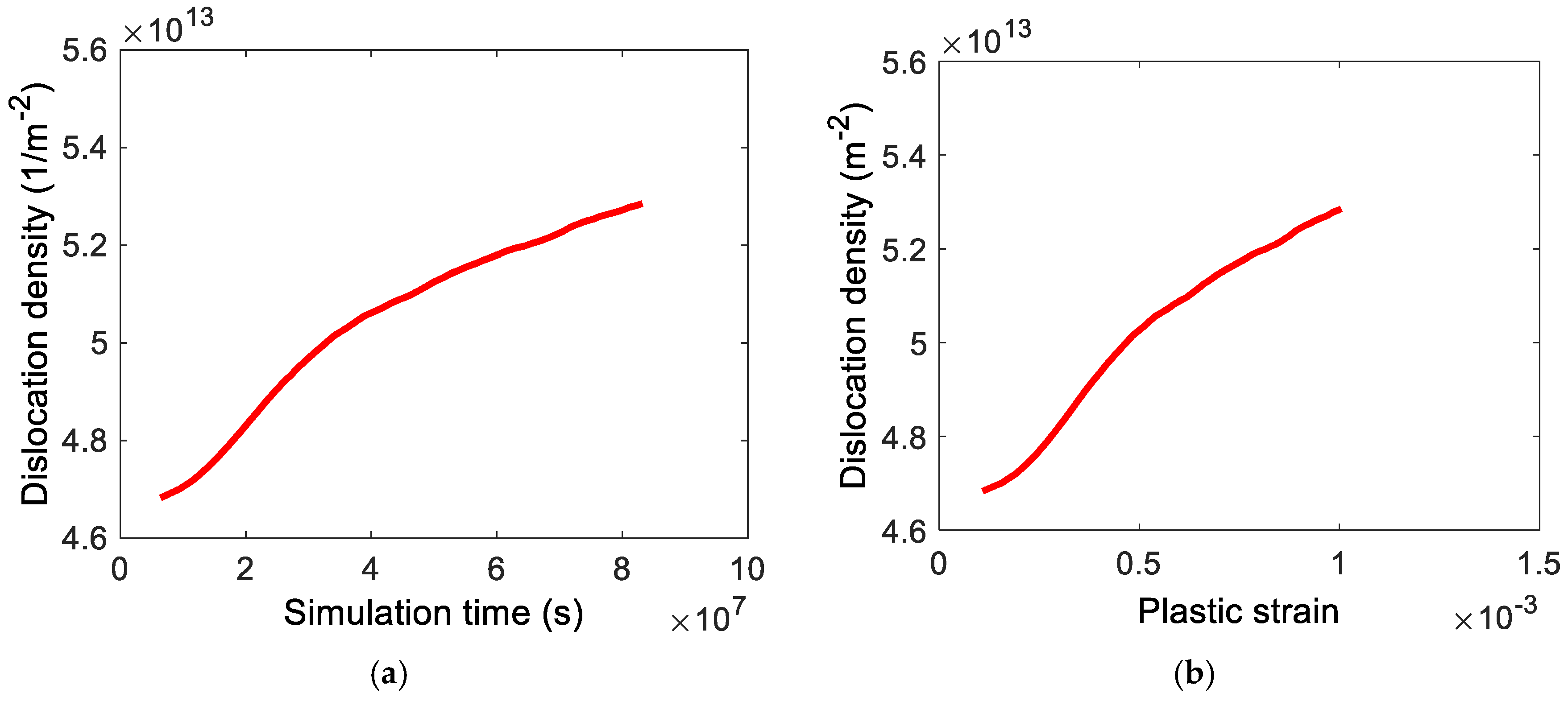
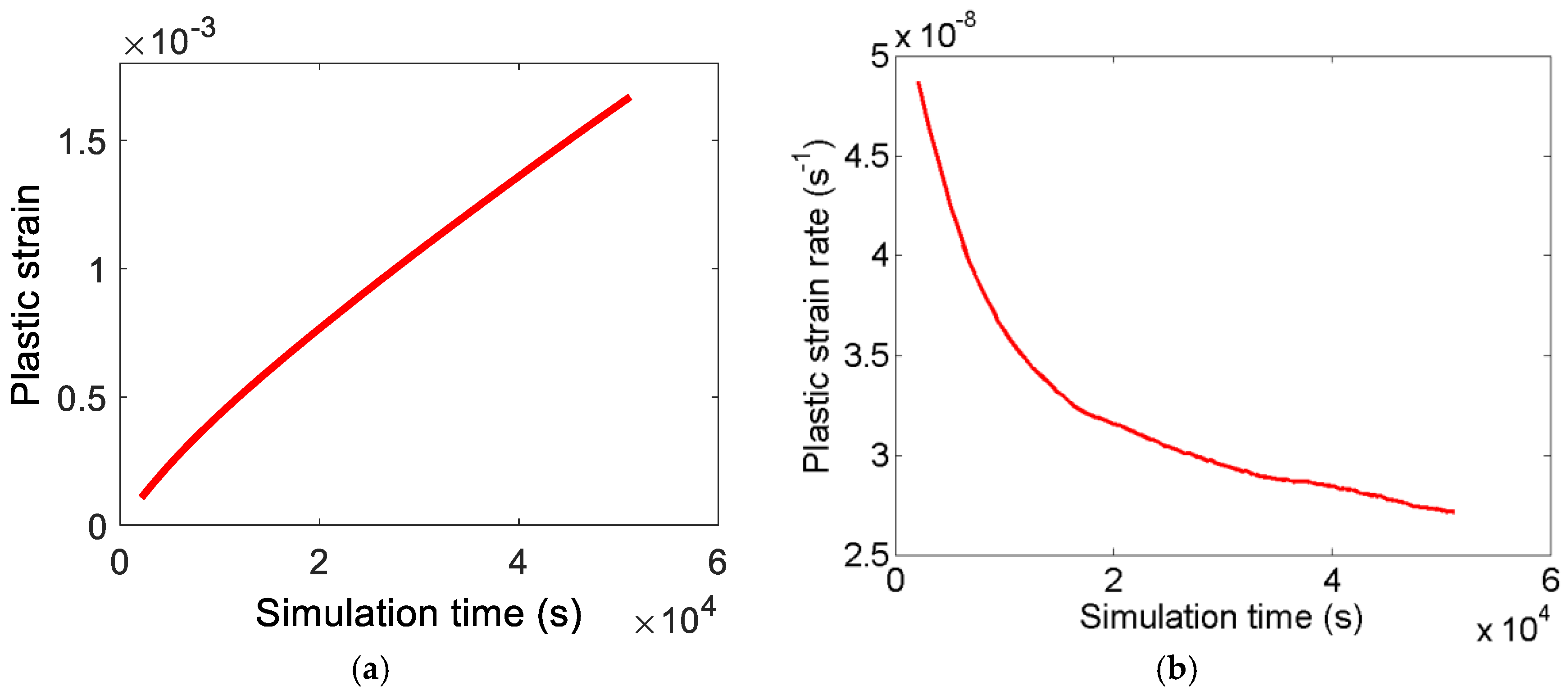
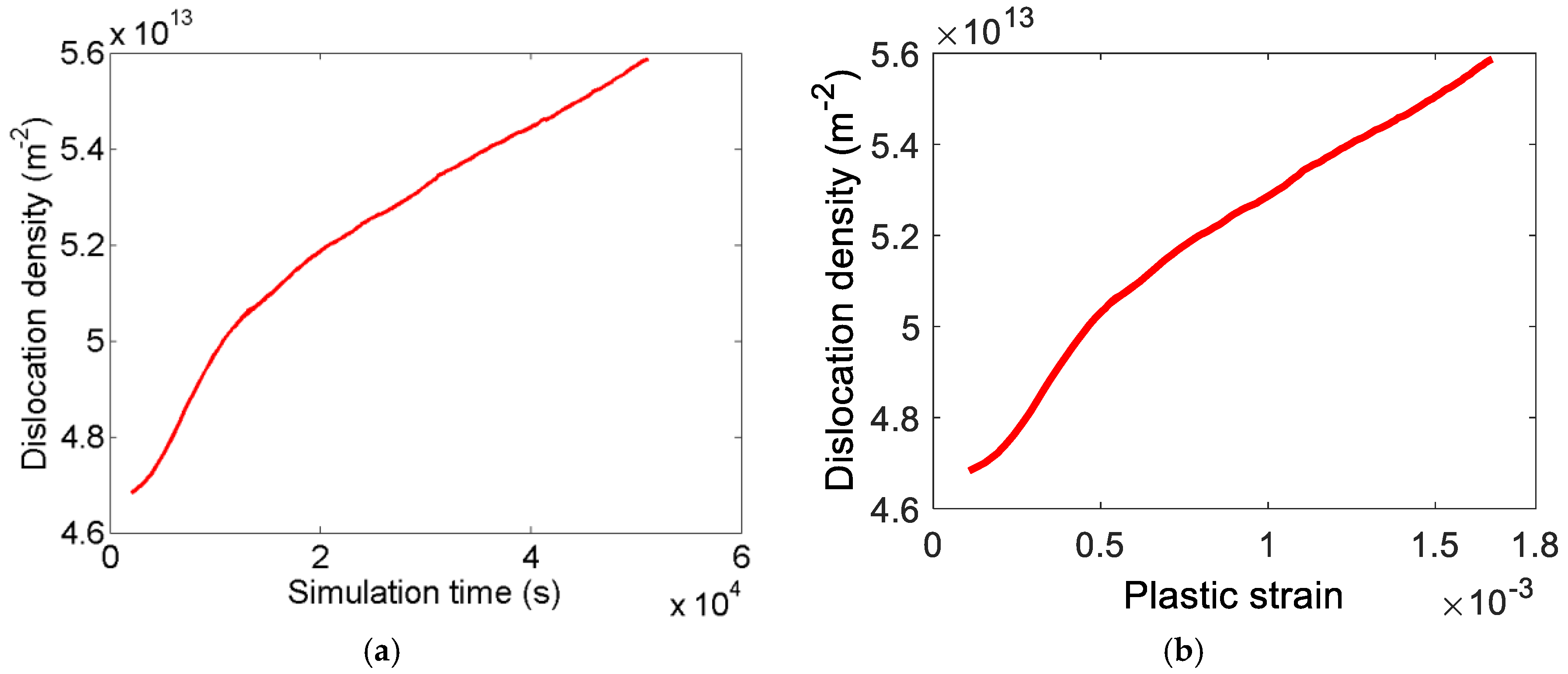
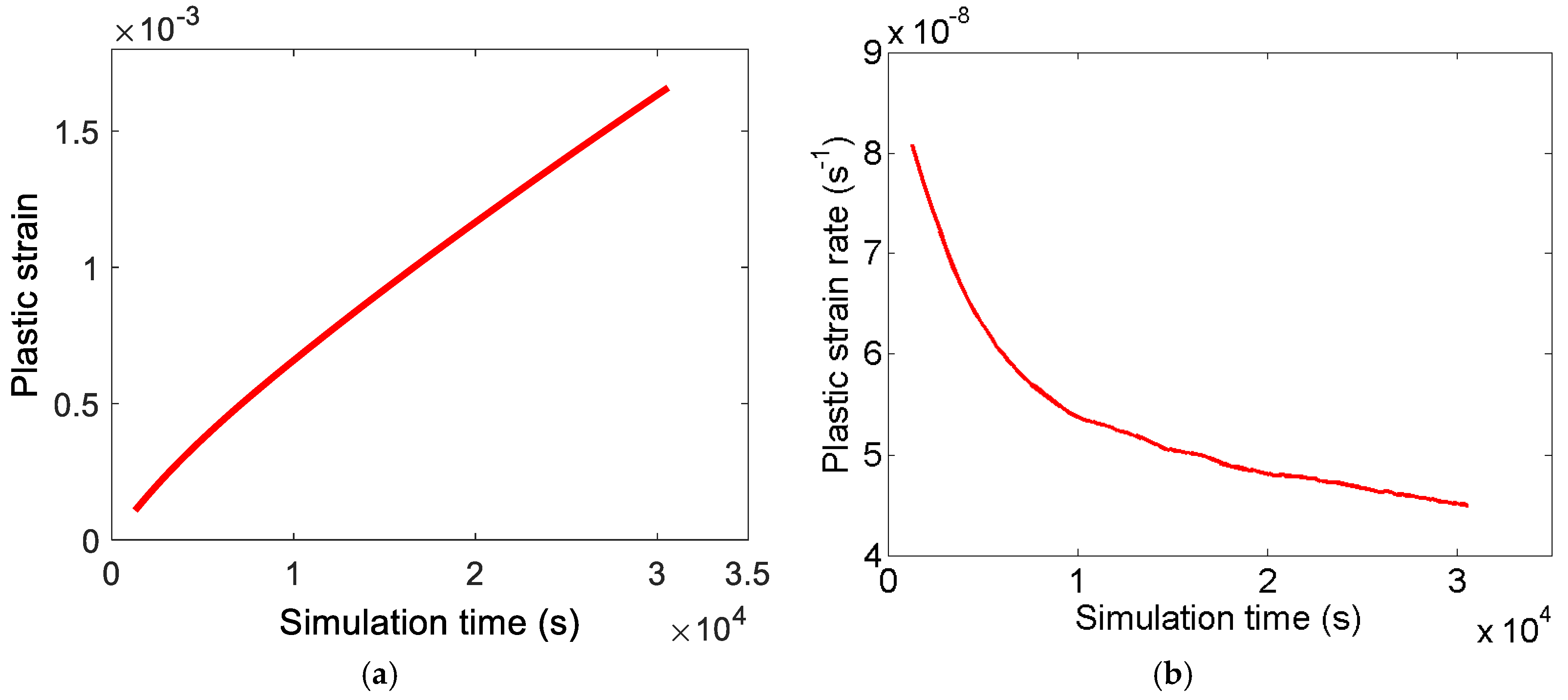
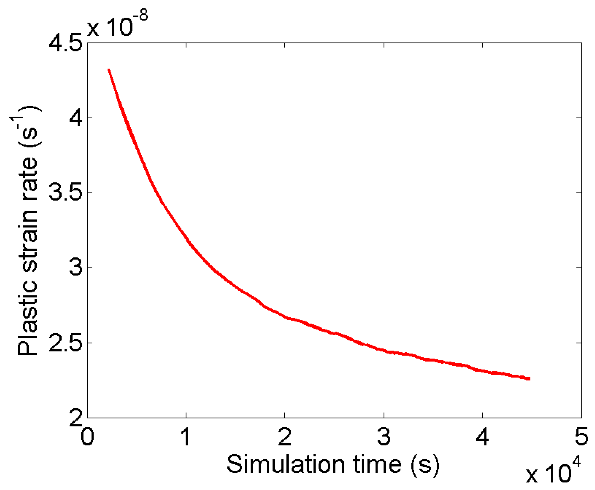
4.2. Dislocation Dynamics Simulation

A three-dimensional dislocation dynamics method was employed to demonstrate how creep deformation of copper at 75 °C can be governed by glide motion of dislocations. To do so, plastic deformation of single-crystal copper was modelled by applying constant tensile stress of σappl = 180 MPa along the [001] direction. Initial dislocation setup consisted of 865 straight dislocations of mixed character randomly distributed inside the cubic simulation volume with an edge length of 5 µm. The simulation box was subjected to three-dimensional period boundary conditions (PBCs) to mimic the bulk material. To resemble a non-deformed crystal, initial dislocation density over the simulation volume was set to ρ0 = 4.1 × 10¹³ m−2.
The material parameters were set for copper as follows, shear modulus G = 42 GPa, Poisson’s ratio ν = 0.31, and Burger vector b = 0.256 nm. Identical drag coefficient B and consequently the same glide mobility were used for both edge and screw dislocations. While screw dislocations may leave their original primary plane and cross slip to a secondary plane, climb motion of edge dislocation was hindered over the course of simulations. Therefore, edge dislocations were mostly confined to their {111} slip planes.
Simulations were performed with three different values of the glide mobility. The first set of simulations were conducted with an original mobility value of Mglide = 2.89 × 10⁻¹³ (Pa·s)−1 and the resultant response of the single-crystal is plotted in Figure 4 as plastic strain and plastic strain rate versus simulation time. There was an almost linear increase in strain with time. Figure 4b shows that the plastic strain rate and the creep rate decreased with time and eventually leveled off at around ε ˙ = 1.0 × 10 11   s 1 . This strain rate is 3 × 10³ times less than the value predicted by Equations (2) and (3).
The development of the dislocation density is shown in Figure 5 as a function of simulation time (a) and plastic strain (b). The dislocation density reached a fairly high value early in the simulation and then continued to grow. The general appearance of Figure 5a,b were similar, since the plastic strain approximately increased linearly with time, see Figure 4a.
To interpret these results, we considered the effective stress σeff, Equation (1). All the dislocations in the simulation generated a stress field. Each individual dislocation was exposed to a combination of these stress fields from surrounding dislocations in addition to the externally applied stress. These combined stress fields are referred to as the internal stress σi. The value of the internal stress can be computed from the simulation. This is analyzed in the next section. The effective stress σeff drives the motion of the dislocations. Since the computed strain rate was much less than the one evaluated from the mobility, it is natural to assume that the effective stress was much lower than the applied stress. To investigate this possibility, a new simulation was made with a mobility that was increased by a factor 3 × 10³, giving a mobility of Mglide = 8.67 × 10⁻¹⁰ (Pa·s)−1. The results of the simulations are shown in Figure 6 and Figure 7.
The strain increases with time in Figure 6a and the strain rate versus time curve in Figure 6b shows a decreasing creep rate with increasing time in the same way as in Figure 4a,b. The dislocation density as a function of plastic strain in Figure 6b has also a similar appearance to that in Figure 5b. The final strain rate in Figure 6b is approximately ε ˙ = 2.7 × 10 8 s 1 . This value is almost identical to that estimated from Equations (2) and (3). Since large strains cannot be obtained in the simulation, a stationary condition was not reached. However, since the variation of the dislocation density as a function of time was modest, Figure 7a, the results can be said to represent a quasi-stationary condition. By employing a higher glide mobility in the second set of calculations, a creep rate close to the ones corresponding to observations was obtained, see Figure 3.
Figure 8a,b shows the results of the third set of simulations where deformation of the single-crystal was modeled with a glide mobility of Mglide = 1.44 × 10⁻⁹ (Pa·s)−1, which represents a further increase of 1.67 in the mobility.
Similar to the previous calculations with lower mobility values in Figure 4 and Figure 6, plastic strain rate decreased during deformation of the single-crystal to finally a constant value of almost ε ˙ = 4.5 × 10 8   s 1 . This was an increase with a factor of 1.67 in comparison with that in Figure 6 (i.e., the same as the increase in the mobility). It is obvious that the predicted creep rate was approximately linear with the mobility in the considered range. It was the purpose of the second increase to demonstrate the linearity. The dislocation density versus time and plastic strain curves are not shown, since their appearance was almost identical to the corresponding curves in Figure 7.
Dislocation dynamics simulation results shown in Figure 4 to Figure 8 demonstrate that single-crystal copper experiences creep deformation only by glide motion of dislocations under constant stress.

5. Evaluation of Effective Stresses

Effective stresses acting on the dislocation lines can be calculated directly using dislocation dynamics simulation results. The existing relation between velocity of dislocations, V, and effective stress, σ eff , acting on dislocations is as follows:
V = M glide σ eff b
where Mglide and b represent the glide mobility and the magnitude of Burgers vector, respectively. The mean value of effective stresses along each of three directions (i.e., x, y and z) is calculated using generated velocity data extracted from the dislocation dynamics results for the three sets of glide mobilities, see Table 1. The external stress is applied in the z direction. Effective stresses are calculated at three stages of deformation: early, intermediate, and final stages corresponding to plastic strains of 0.02%, 0.06%, and maximum computed strain. The absolute values of effective stresses are in general more than three orders of magnitude smaller than the applied stress. The amount of scatter in the results can be estimated from the average values in the x and y directions, which should be zero.
It is obvious that the scatter in the values is many times larger than the estimated effective stress in the section on glide controlled creep that was 180 × 106/3000 = 0.6 × 10⁵ Pa. From Table 1, one can conclude that the true value of the effective stress is not larger than the estimated value 0.6 × 10⁵ Pa.

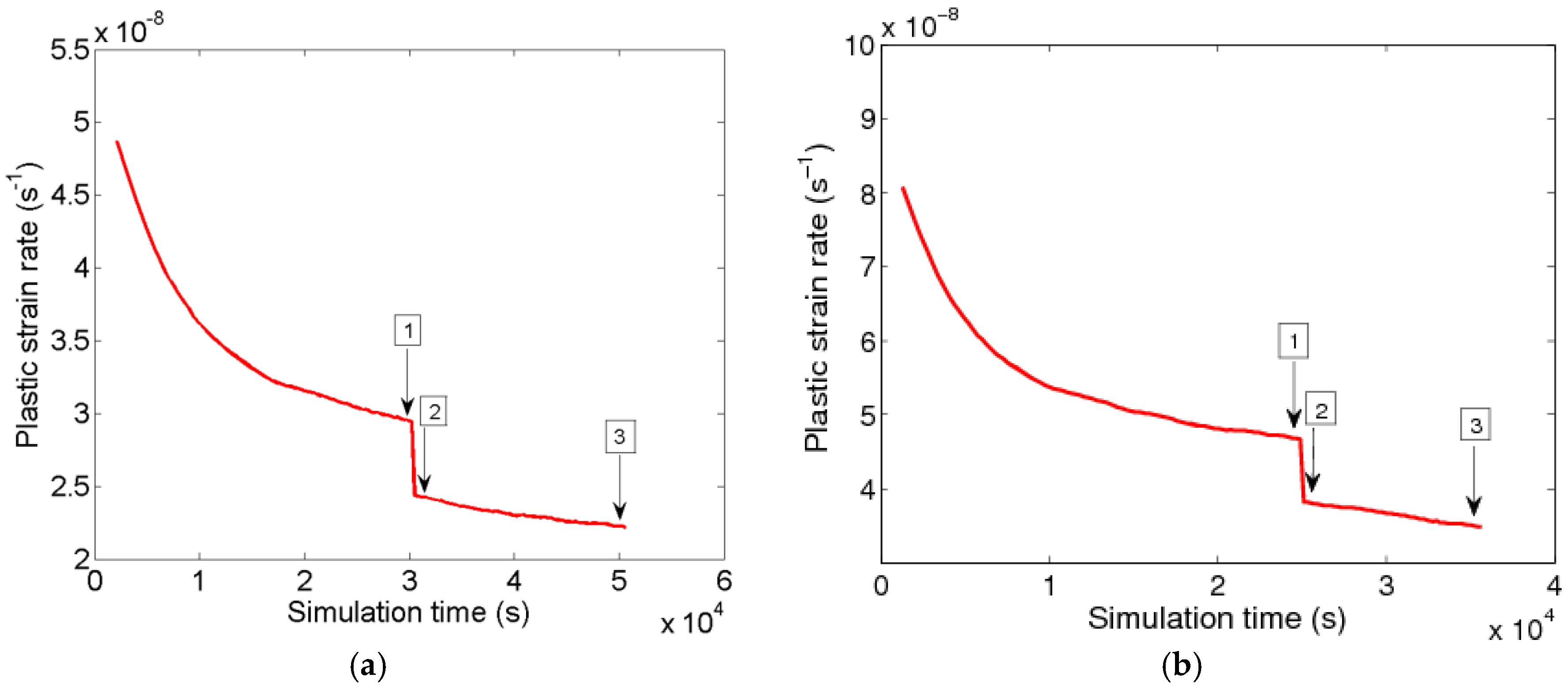
6. Effect of Change in the Applied Stress

In this section, the effect of a rapid change in the applied creep stress on the stress acting on dislocations (i.e., effective stress) is examined. To do so, the applied stress is instantly reduced from 180 MPa to 160 MPa during plastic deformation. In the first stage of deformation, the single-crystal undergoes creep deformation at constant stress level of 180 MPa and in the second stage the material deforms at a lower stress level of 160 MPa. In Figure 9, the influence of the stress change on the strain rate is illustrated. The same glide mobilities of Mglide = 8.67 × 10⁻¹⁰ (Pa·s)−1 and Mglide = 1.44 × 10⁻⁹ (Pa·s)−1 as in the section on glide controlled creep were used. The plastic strain rate exhibited an abrupt reduction as the applied stress changed from 180 to 160 MPa.
In Figure 10, the strain rate versus time at the lower stress 160 MPa is shown. The results in Figure 9a after the stress drop and in Figure 10 at the corresponding times were very close. Obviously, the effect of the previous deformation was weak.
Evaluation of effective stresses acting on dislocations is performed at the three illustrated points in Figure 9. Point 1 corresponds to the first stage, i.e., σappl = 180 MPa, and points 2 and 3 correspond to the second stage of deformation, i.e., σappl = 160 MPa. Table 2 shows predicted mean effective stresses acting on dislocation lines along each of three x, y, and z directions at three illustrated points in Figure 9a,b.
The scatter in the average effective stresses in Table 2 is of the same order as in Table 1. This means that the internal stress is at the same level as the applied stress also directly after the stress change. Thus, there is no evidence that the internal stress has any direct memory of the earlier applied stress.

7. Discussion

A fundamental expression for the climb mobility of dislocations, Equation (7), has been available for a long time [3]. A corresponding basic expression for glide has not been possible to find. Instead, a number of authors have used the empirical expression in Equation (8) or a similar one from Reference [26]. Since it involves a number of unknown constants, it cannot be used for making predictions. As described in section on the creep mobility, to solve this problem a unified climb and glide mobility was set up. This immediately fixed some of the unknown constants and the remainder of the parameters could be chosen by general arguments. The resulting semi-empirical expression has successfully been used in a number of publications for different applications.
In the present paper, the semi-empirical model was analyzed by deriving the glide rate at low temperatures. It was assumed that the glide rate is controlled by the climb rate of jogs on the dislocations. At low temperatures, the climb rate is enhanced by an excess concentration of vacancies that is generated during the creep deformation. The derived glide rate is almost identical to the results from the semi-empirical glide mobility, Figure 1 and Figure 2, which fully verifies this expression for the glide mobility. It is possible to verify the validity of Equation (10) in an alternative way by relating it more directly to the climb rate [10,11].
Using the (verified) expression for glide mobility, creep deformation has been simulated with the help of dislocation dynamics. In these simulations, glide and cross glide have been taken into account, but not climb. Although it has not been possible to reach more than about 0.1% strain in the simulation, an apparent quasi-stationary condition with a fairly constant dislocation density was reached. The simulations show that pure glide can give rise to creep at low temperatures, which has been assumed in the literature for a number of years, see for example References [1,4].
In modelling creep deformation, a back stress or internal stress is often assumed. Many authors have considered the back stress in pure metals to be a physical quantity that can be measured with the help of stress drop tests, see for example References [14,34]. However, from the dislocation dynamics simulations one finds that the internal stress is almost identical to the applied stress. It was demonstrated that this is the case even directly after a stress drop. A direct measurement of the internal stress is then not possible. The concept of back stress can still be useful. It can be defined in many ways. But, it is not accessible to direct measurement, and many authors have realized this, see for example References [12,35]. The investigated situation does not cover the case when a stable substructure is present, which may take a longer time to relax. This is for example the case in 9% Cr-steels, where the sub-boundaries are stabilized by M23C6 carbides [36].

8. Conclusions

The glide rate of dislocations in copper at low temperatures is much higher than the climb rate. The glide rate has been derived based on the assumption that it is controlled by the climb of the jogs on the dislocations. The derived expression for the glide rate is in good accordance with a previously presented semi-empirical expression for the glide mobility.
This gives a fundamental understanding of the controlling creep mechanisms at near ambient temperatures, which is essential for example for the application of copper in canisters for disposal of spent nuclear waste.
Low temperature creep in copper has been simulated with dislocation dynamics (DD) taking glide but not climb into account. In the DD simulation a plastic strain of about 0.1% was reached. In spite of the low strain, the strain rate and the dislocation density reached an apparent quasi-stationary condition. It supports that creep at low temperatures can be controlled by glide alone.
Each dislocation in the DD simulations was exposed to an internal stress from surrounding dislocations. In the load direction, the internal stress was almost equal to the applied stress. In the investigated case, the difference between the applied and the internal stress, the effective stress, was only 1/3000 of the applied stress. This was taken into account in the simulation.
The effect of stress drop in the simulations was investigated. It turned out that the effective stress directly after the stress drop was as small as at constant stress. Obviously, the internal stress immediately adapts to the new stress level.

Author Contributions

A.H.D. performed the DD simulations, R.S. developed the dislocation mobility model, A.H.D., R.S. and P.K. wrote the paper.

Acknowledgments

The author would like to thank the Swedish Nuclear Fuel and Waste Management Co (SKB) for funding this work, contract 9114. Computer resources for this study at PDC Center for High Performance Computing at the KTH Royal Institute of Technology in Stockholm and National Supercomputer Center (NSC) at Linköping University were provided by the Swedish National Infrastructure for Computing (SNIC, projects 2014/11-25, 2015/16-50 and 2016/34-51).

Conflicts of Interest

The authors declare no conflict of interest.

Appendix A. Parameter Values Used in the Computations

Table A1. Values and interpretation of constants.
Parameter DescriptionParameterValueReference
Coefficient for self-diffusionDs01.31 × 10−5 m2/s[37]
Activation energy for self-diffusionQ198,000 J/mol[37]
Burgers vectorb2.56 × 10−10 m
Atomic volumeΩ0 b 3 / 2 = 1.18× 10⁻²⁹ m3
Lattice misfit for P atomε0.055[22]
Taylor factorm3.06
Constant in Taylor’s equation describing the influence of dislocation density on the strengthα(1 − ν/2)/2π(1 − ν) = 0.19[38,39]
Max back stressσimax257 MPa[1]
Dislocation line tensionτLGb2/2 = 7.94∙× 10−16 MN
Subgrain stress constantKsub11[40]
Max interaction energy between P solute and dislocation U P max 8220 J/mol[22]
Boltzmann’s constantkB1.381 × 10−23 J/grad
Grain sizedgrain100 μm[2]
Shear modulusG45,400 × (1 − 7.1 × 10⁻⁴ × (T − 20)), MPa, T in °C[41]
Yield strengthσy75 MPa for as hot worked in reference condition. For value at other temperatures and strain rates, see Ref.[19]
Work hardening constantcL28–31[19]

References

  1. Sandstrom, R.; Andersson, H.C.M. Creep in phosphorus alloyed copper during power-law breakdown. J. Nucl. Mater. 2008, 372, 76–88. [Google Scholar] [CrossRef]
  2. Sandstrom, R. Basic model for primary and secondary creep in copper. Acta Mater. 2012, 60, 314–322. [Google Scholar] [CrossRef]
  3. Hirth, J.P.; Lothe, J. Theory of Dislocations; Krieger: Malabar, FL, USA, 1982. [Google Scholar]
  4. Blum, W.; Rosen, A.; Cegielska, A.; Martin, J.L. Two mechanisms of dislocation motion during creep. Acta Metall. 1989, 37, 2439–2453. [Google Scholar] [CrossRef]
  5. Kocks, U.F. A statistical theory of flow stress and work-hardening. Philos. Mag. 1966, 13, 541–566. [Google Scholar] [CrossRef]
  6. Lagneborg, R. Dislocation mechanisms in creep. Int. Metall. Rev. 1972, 17, 130–146. [Google Scholar]
  7. Sandström, R. The role of cell structure during creep of cold worked copper. Mater. Sci. Eng. A 2016, 674, 318–327. [Google Scholar] [CrossRef]
  8. Cottrell, A.H. Logarithmic and andrade creep. Philos. Mag. Lett. 1997, 75, 301–307. [Google Scholar] [CrossRef]
  9. Nabarro, F.R.N. The time constant of logarithmic creep and relaxation. Mater. Sci. Eng. A 2001, 309–310, 227–228. [Google Scholar] [CrossRef]
  10. Spigarelli, S.; Sandström, R. Basic creep modelling of aluminium. Mater. Sci. Eng. A 2018, 711, 343–349. [Google Scholar] [CrossRef]
  11. Sandström, R. Fundamental Modelling of Creep Properties. In Creep; Tanski, T., Zieliński, A., Eds.; inTech: London, UK, 2017. [Google Scholar]
  12. Biberger, M.; Gibeling, J.C. Analysis of creep transients in pure metals following stress changes. Acta Metall. Mater. 1995, 43, 3247–3260. [Google Scholar] [CrossRef]
  13. Chen, B.; Flewitt, P.E.J.; Cocks, A.C.F.; Smith, D.J. A review of the changes of internal state related to high temperature creep of polycrystalline metals and alloys. Int. Mater. Rev. 2015, 60, 1–29. [Google Scholar] [CrossRef]
  14. Ahlquist, C.N.; Nix, W.D. The measurement of internal stresses during creep of al and Al-Mg alloys. Acta Metall. 1971, 19, 373–385. [Google Scholar] [CrossRef]
  15. Cuddy, L.J. Internal stresses and structures developed during creep. Metall. Mater. Trans. B 1970, 1, 395–401. [Google Scholar] [CrossRef]
  16. Davies, P.W.; Williams, K.R. Cavity growth by grain-boundary sliding during creep of copper. Met. Sci. 1969, 3, 220–221. [Google Scholar] [CrossRef]
  17. Henderson, P.J.; Sandstrom, R. Low temperature creep ductility of OFHC copper. Mater. Sci. Eng. A 1998, 246, 143–150. [Google Scholar] [CrossRef]
  18. Sandström, R.; Wu, R. Influence of phosphorus on the creep ductility of copper. J. Nucl. Mater. 2013, 441, 364–371. [Google Scholar] [CrossRef]
  19. Sandström, R.; Hallgren, J. The role of creep in stress strain curves for copper. J. Nucl. Mater. 2012, 422, 51–57. [Google Scholar] [CrossRef]
  20. Sandström, R. Fundamental Models for Creep Properties of Steels and Copper. Trans. Indian Inst. Met. 2016, 69, 197–202. [Google Scholar] [CrossRef]
  21. Wu, R.; Sandström, R.; Jin, L.Z. Creep crack growth in phosphorus alloyed oxygen free copper. Mater. Sci. Eng. A 2013, 583, 151–160. [Google Scholar] [CrossRef]
  22. Sandstrom, R.; Andersson, H.C.M. The effect of phosphorus on creep in copper. J. Nucl. Mater. 2008, 372, 66–75. [Google Scholar] [CrossRef]
  23. Sandström, R. Influence of phosphorus on the tensile stress strain curves in copper. J. Nucl. Mater. 2016, 470, 290–296. [Google Scholar] [CrossRef]
  24. Korzhavyi, P.A.; Sandström, R. First-principles evaluation of the effect of alloying elements on the lattice parameter of a 23Cr25NiWCuCo austenitic stainless steel to model solid solution hardening contribution to the creep strength. Mater. Sci. Eng. A 2015, 626, 213–219. [Google Scholar] [CrossRef]
  25. Nes, E.; Marthinsen, K. Modeling the evolution in microstructure and properties during plastic deformation of f.c.c.-metals and alloys—An approach towards a unified model. Mater. Sci. Eng. A 2002, 322, 176–193. [Google Scholar] [CrossRef]
  26. Kocks, U.F.; Argon, A.S.; Ashby, M.F. Thermodynamics and kinetics of slip. Prog. Mater. Sci. 1975, 19, 291. [Google Scholar]
  27. Chandler, H.D. Effect of unloading time on interrupted creep in copper. Acta Metall. Mater. 1994, 42, 2083–2087. [Google Scholar] [CrossRef]
  28. Mecking, H.; Estrin, Y. The effect of vacancy generation on plastic deformation. Scr. Metall. 1980, 14, 815–819. [Google Scholar] [CrossRef]
  29. Sandström, R. The role of microstructure in the prediction of creep rupture of austenitic stainless steels. In Proceedings of the ECCC Creep & Fracture Conference, Düsseldorf, Germany, 10–14 September 2017. [Google Scholar]
  30. Arsenlis, A.; Cai, W.; Tang, M.; Rhee, M.; Oppelstrup, T.; Hommes, G. Enabling strain hardening simulations with dislocation dynamics. Model. Simul. Mater. Sci. Eng. 2007, 15, 553–595. [Google Scholar] [CrossRef] [Green Version]
  31. Haghighat, S.M.H.; Eggeler, G.; Raabe, D. Effect of climb on dislocation mechanisms and creep rates in γ′-strengthened Ni base superalloy single crystals: A discrete dislocation dynamics study. Acta Mater. 2013, 61, 3709–3723. [Google Scholar] [CrossRef]
  32. Delandar, A.H.; Haghighat, S.M.H.; Korzhavyi, P.; Sandström, R. Dislocation dynamics modeling of plastic deformation in single-crystal copper at high strain rates. Int. J. Mater. Res. 2016, 107, 988–995. [Google Scholar] [CrossRef]
  33. Bulatov, V.V.; Cai, W. Computer Simulations of Dislocations; Oxford University Press: Oxford, UK, 2006. [Google Scholar]
  34. Matsuo, T.; Nakajima, K.; Terada, Y.; Kikuchi, M. High temperature creep resistance of austenitic heat-resisting steels. Mater. Sci. Eng. A 1991, 146, 261–272. [Google Scholar] [CrossRef]
  35. Hausselt, J.; Blum, W. Dynamic recovery during and after steady state deformation of Al-11wt%Zn. Acta Metall. 1976, 24, 1027–1039. [Google Scholar] [CrossRef]
  36. Magnusson, H.; Sandstrom, R. Creep strain modeling of 9 to 12 Pct Cr steels based on microstructure evolution. Metall. Mater. Trans. A 2007, 38, 2033–2039. [Google Scholar] [CrossRef]
  37. Neumann, G.; Tölle, V.; Tuijn, C. Monovacancies and divacancies in copper Reanalysis of experimental data. Phys. B Condens. Matter 1999, 271, 21–27. [Google Scholar] [CrossRef]
  38. Horiuchi, R.; Otsuka, M. Mechanism of high temperature creep of aluminum-magnesium solid solution alloys. Trans. Jpn. Inst. Met. 1972, 13, 284–293. [Google Scholar] [CrossRef]
  39. Orlová, A. On the relation between dislocation structure and internal stress measured in pure metals and single phase alloys in high temperature creep. Acta Metall. Mater. 1991, 39, 2805–2813. [Google Scholar] [CrossRef]
  40. Wu, R.; Pettersson, N.; Martinsson, Å.; Sandström, R. Cell structure in cold worked and creep deformed phosphorus alloyed copper. Mater. Charact. 2014, 90, 21–30. [Google Scholar] [CrossRef]
  41. Ledbetter, H.M.; Naimon, E.R. Elastic Properties of Metals and Alloys. II. Copper. J. Phys. Chem. Ref. Data 1974, 3, 897–935. [Google Scholar] [CrossRef]
Figure 1. Comparison of the deformation induced increase in the vacancy concentration gglide, Equation (19), that raises the climb rate with the expression for the climb glide enhancement factor fenh, Equation (10). Results are presented for Cu-OFP at four strain rates.
Metals 08 00772 g001
Figure 2. Comparison of the deformation induced increase in the vacancy concentration gclimb, Equation (19), that raises the glide rate with the expression for the climb glide enhancement factor fenh, Equation (10). Results are presented for Cu-OFP at six temperatures.
Metals 08 00772 g002
Figure 3. Predicted secondary creep rate with the dislocation mobility in Equation (9).
Metals 08 00772 g003
Figure 4. (a) Plastic strain and (b) plastic strain rate versus simulation time for deformation with the original mobility value Mglide = 2.89 × 10⁻¹³ (Pa·s)−1.
Metals 08 00772 g004
Figure 5. Dislocation density versus (a) simulation time and (b) plastic strain for deformation with original mobility value Mglide = 2.89 × 10⁻¹³ (Pa·s)−1.
Metals 08 00772 g005
Figure 6. (a) Plastic strain and (b) plastic strain rate versus simulation time for Mglide = 8.67 × 10⁻¹⁰ (Pa·s)−1.
Metals 08 00772 g006
Figure 7. Dislocation density versus (a) simulation time and (b) plastic strain for deformation with the mobility value Mglide = 8.67 × 10⁻¹⁰ (Pa·s)−1.
Metals 08 00772 g007
Figure 8. (a) Plastic strain and (b) plastic strain rate versus simulation time for Mglide = 1.44 × 10⁻⁹ (Pa·s)−1.
Metals 08 00772 g008
Figure 9. Abrupt change in plastic strain rate when the applied stress was reduced from 180 MPa to 160 MPa; (a) Mglide = 8.67 × 10⁻¹⁰ (Pa·s)−1; (b) Mglide = 1.44 × 10⁻⁹ (Pa·s)−1.
Metals 08 00772 g009
Figure 10. Plastic strain rate versus simulation time for deformation at stress level of σappl = 160 MPa and with mobility value of Mglide = 8.67 × 10⁻¹⁰ (Pa·s)−1.
Metals 08 00772 g010
Table 1. Calculated mean value of effective stresses along x, y, and z directions at three stages of deformation.
Mglide (Pa·s)−1Three Stages of Deformation σ ¯ effx ( Pa ) σ ¯ effy ( Pa ) σ ¯ effz ( Pa )
2.89 × 10⁻¹³Early1.22 × 105−0.92 × 1050.81 × 105
Intermediate0.09 × 105−1.96 × 1050.89 × 105
Final−0.61 × 10⁵−1.58 × 1050.54 × 105
8.67 × 10⁻¹⁰Early1.29 × 105−1.12 × 1051.01 × 105
Intermediate−0.86 × 10⁵−0.71 × 1050.81 × 105
Final−0.82 × 10⁵−1.45 × 10⁵−2.39 × 10⁵
1.44 × 10⁻⁹Early1.32 × 105−1.15 × 1050.85 × 105
Intermediate0.40 × 105−0.71 × 10⁵−0.41 × 10⁵
Final−1.06 × 10⁵−0.61 × 10⁵−1.42 × 10⁵
Table 2. The calculated mean effective stresses at the three illustrated points in Figure 9.
Mglide (Pa·s)−1Illustrated Points σ ¯ effx ( Pa ) σ ¯ effy ( Pa ) σ ¯ effz ( Pa )
8.67 × 10−101−0.86 × 10⁵−0.71 × 10⁵−0.81 × 10⁵
2−0.39 × 10⁵−0.92 × 10⁵−0.33 × 10⁵
3−1.06 × 10⁵−0.72 × 10⁵−1.84 × 10⁵
1.44 × 10−91−1.57 × 10⁵−1.15 × 10⁵−1.47 × 10⁵
2−0.73 × 10⁵−0.75 × 10⁵−0.54 × 10⁵
3−1.18 × 10⁵−0.96 × 10⁵−1.95 × 10⁵

