A Hybrid Multi-Scale Model of Crystal Plasticity for Handling Stress Concentrations

Abstract

Microstructural effects become important at regions of stress concentrators such as notches, cracks and contact surfaces. A multiscale model is presented that efficiently captures microstructural details at such critical regions. The approach is based on a multiresolution mesh that includes an explicit microstructure representation at critical regions where stresses are localized. At regions farther away from the stress concentration, a reduced order model that statistically captures the effect of the microstructure is employed. The statistical model is based on a finite element representation of the orientation distribution function (ODF). As an illustrative example, we have applied the multiscaling method to compute the stress intensity factor ${\mathit{K}}_I$ around the crack tip in a wedge-opening load specimen. The approach is verified with an analytical solution within linear elasticity approximation and is then extended to allow modeling of microstructural effects on crack tip plasticity.

1. Introduction

Efficient micro-scale modeling tools are needed to compute microstructure-dependent properties of advanced structural alloys used in aerospace, naval and automotive applications [1]. Microstructural effects become an important consideration in regions of stress concentrations such as notches, cracks and contact surfaces. While the crystal plasticity finite element (CPFE) method has emerged as an effective tool for simulating the mechanical response of aggregates of a few hundred metallic crystals, the simulation of ‘macro-scale’ components that contain millions of grains is a challenging task even when using current state-of-the-art supercomputers. Multiscale methods developed to address this problem can be broadly classified into two categories: concurrent and hierarchical methods. In hierarchical methods, the objective is to obtain material properties of a coarse-scale model by simulating a fine-scale model that contains features smaller than those allowed by the coarse-scale mesh resolution. A popular example is the computational homogenization approach [2,3] where volume averaging schemes are employed to extract macroscale properties.

In concurrent methods, both fine- and coarse-scale problems are solved together in a single domain using multi-resolution meshes. Most popular among these methods are quasicontinuum methods, where the resolution of meshes from atomistic to continuum scales has been considered to study crack propagation [4]. In QC methods, the treatment of interfaces between fine- and coarse-scale regions becomes problematic when multi-physical domains (e.g., crystal plasticity at the fine scale and continuum plasticity at the coarse scale) are considered. For example, Dunne et al. (2007) [5] employed a combined continuum crystal plasticity finite element approach for modeling a three-point bend test. One of the potential difficulties identified in the model was the inconsistency of yield stress at the interface between the domains. To minimize the effect, the choice of the critical resolved shear stress in the crystal plasticity model was made such that polycrystal yielding occurred at a value close to the continuum yield stress.

In this paper, the interface problem is solved through the use of a single physical model at both the fine and coarse scales. This is achieved (i) by explicitly resolving single-crystal deformation at the fine scale (crack tip) using a crystal plasticity model and (ii) by employing a hierarchical multiscale model at the coarse scale (far region), where polycrystal aggregates are homogenized using the same crystal plasticity model. While the method combines the best aspects of both hierarchical and concurrent methods, it is still computationally expensive to model polycrystalline aggregates at every coarse-scale material point.

An alternate class of schemes has been developed in recent years that allows the representation of microstructure using probabilistic descriptors. The simplest of these descriptors is the one-point probability measure, the orientation distribution function ($\mathcal{A}\left(\mathit{g}\right)$), which quantifies the volume fractions of crystals in the orientation space (g). Under an applied deformation, texturing is simulated by numerically evolving the orientation distribution function (ODF) (rather than the microstructure itself) using conservation laws [6]. A variety of ODFs can be represented over a finite element (FE) mesh of the orientation space that has significantly lower degrees of freedom when compared to a microstructure FE mesh [7,8,9]. For example, individual crystals close to the crack tip can be modeled using an ODF that is a delta function in the orientation space. Farther from the notch tip, smoothly varying ODFs can be modeled over an uniform grid. The overall multi-scale model is shown in Figure 1. Here, the transition from the microscale to the macroscale is managed through adaptive meshing methods where element lengths can vary from micrometers at the critical regions to as large as several centimeters at the scale of the macroscale component. As an illustrative example, we have applied the multiscaling method to a well-studied problem in fracture mechanics: the computation of the stress intensity factor ${\mathit{K}}_I$ around the crack tip in a wedge-opening load specimen [10]. The multiscale model is subsequently used to analyze the effect of the microstructure at the crack tip when crystal plasticity effects are included. The paper is arranged as follows: In Section 2, the statistical representation of the microstructure is briefly explained, followed by the single-crystal constitutive model. In Section 3, the macro-scale finite element solution procedure is explained. In Section 4, an illustrative example of the approach is provided, followed by conclusions in Section 5.

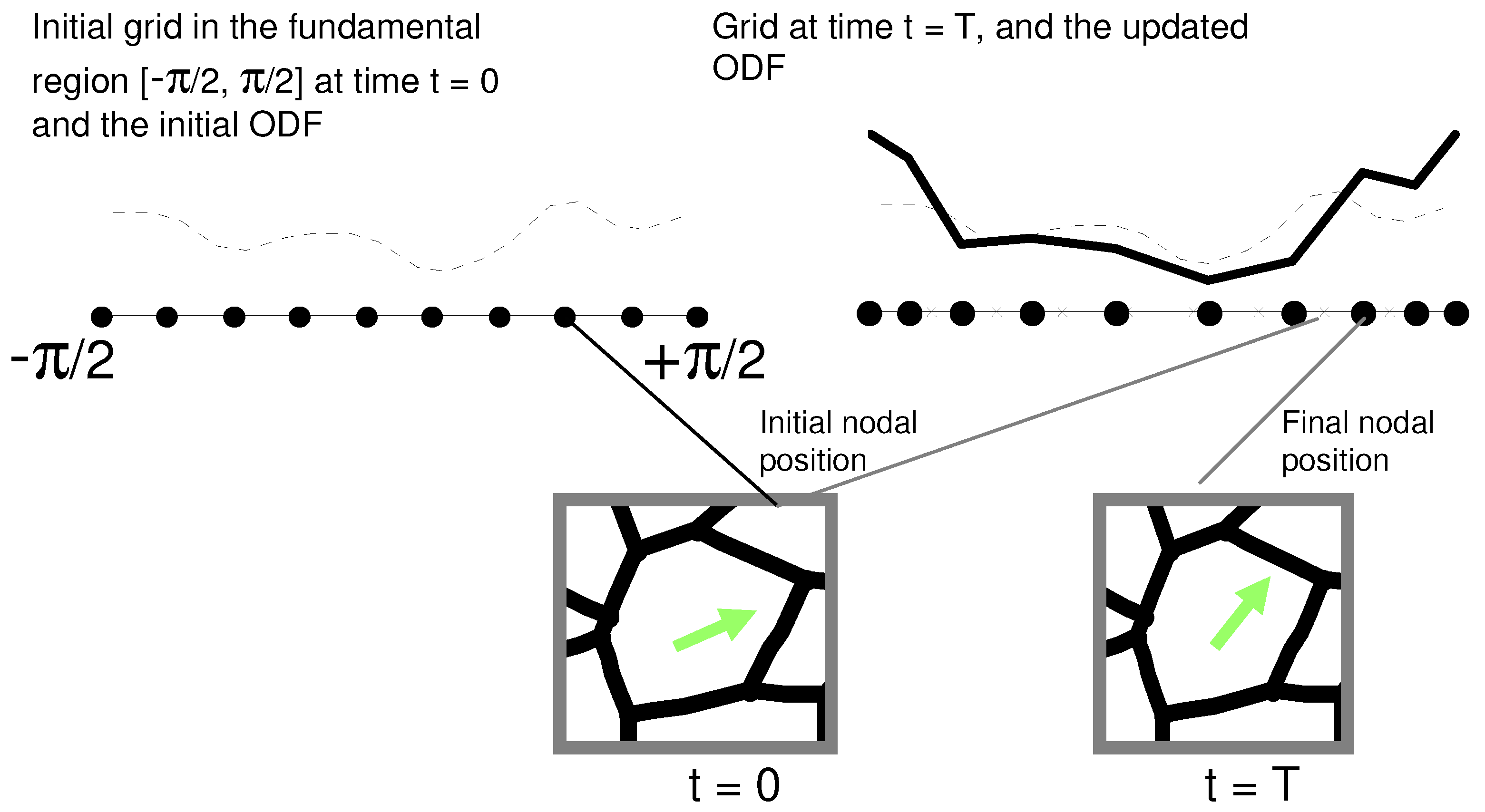
2. Representation of the ODF

The orientation distribution function (ODF, $\mathcal{A}\left(\mathit{g}\right)$) gives the probability density of finding an orientation g in the microstructure. The ODF satisfies the following conservation equations at all times during deformation:

$$\begin{array}{ccc}\hfill \int \mathcal{A}(\mathit{g})d\mathit{g}& =& 1\left(\mathrm{with}\mathcal{A}\right(\mathit{g})\ge 0)\hfill \end{array}$$

(1)

where $d\mathit{g}$ is a differential volume element (the invariant measure) of the orientation space. In addition to the above constraints, the orientation space corresponding to all possible g’s must satisfy the crystallographic symmetries of the chosen system (FCC, HCP, etc.). The complete orientation space of a polycrystal can be reduced to a smaller subset, called the fundamental region, as a consequence of crystal symmetries. Within the fundamental region, each crystal orientation is represented uniquely by the coordinate g, the parametrization for the rotation (e.g., Euler angles, Rodrigues vector etc.). The ODF ($\mathcal{A}\left(\mathit{g}\right)$) can be represented as a probability density function over the fundamental region of orientation space. In this work, a finite element (FE) mesh is used to model the fundamental region, and the ODF is defined at the nodal points of this mesh [8,9]. The probability values between nodal points are obtained as a result of interpolation using finite element shape functions.

2.1. Probability Update in Finite Element Spaces

The probabilities are evolved from time $t=0$ from an initial ODF that satisfies the conservation equations in Equation (1) using a Lagrangian finite element approach [6,7]. The initial orientation ${\mathit{g}}_o$ of a crystal reorients during deformation and maps to a new orientation ${\mathit{g}}_t$ at time t. Simultaneously, the finite element mesh of fundamental region $M_g$ deforms with nodes located at ${\mathit{g}}_o$ moving to new locations ${\mathit{g}}_t$. We assume that the mapping from ${\mathit{g}}_o$ to ${\mathit{g}}_t$ is invertible.

The ODF $\mathcal{A}\left({\mathit{g}}_t\right)$ represents the probability density of crystals with orientation ${\mathit{g}}_t$ at time t. The evolution of the ODF is given by the conservation Equation (1) as:

$$\begin{array}{c}\hfill \int \mathcal{A}({\mathit{g}}_o,t=0)d{\mathit{g}}_o=\int \mathcal{A}\left({\mathit{g}}_t\right)d{\mathit{g}}_t=1\end{array}$$

(2)

where $d{\mathit{g}}_o$ represents the volume element in the undeformed (initial) ODF mesh ($M_{g_o}$), which becomes volume element $d{\mathit{g}}_t$ at time t. A Jacobian $J_F({\mathit{g}}_o,t)=\det \left(\mathit{G}\right)$ gives the ratio of elemental volumes such that $d{\mathit{g}}_t=J_F({\mathit{g}}_o,t)d{\mathit{g}}_o$, where G is the reorientation gradient given as $\mathit{G}({\mathit{g}}_o,t)=\frac{\partial {\mathit{g}}_t}{\partial {\mathit{g}}_o}$. Using the Jacobian, a map of the current mesh (at time t) to the reference mesh (at $t=0$) can be made:

$$\int (\mathcal{A}({\mathit{g}}_o,t=0)-\widehat{\mathcal{A}}({\mathit{g}}_o,t)J_F({\mathit{g}}_o,t))d{\mathit{g}}_o=0$$

(3)

The quantity written as $\widehat{\mathcal{A}}({\mathit{g}}_o,t)$ is the volume density $\mathcal{A}\left({\mathit{g}}_t\right)$ plotted over the corresponding orientation (${\mathit{g}}_o$) in the initial mesh. Thus, $\widehat{\mathcal{A}}({\mathit{g}}_o,t)$ gives the Lagrangian representation of the current ODF in the initial mesh $M_{g_o}$. If the integrand is continuous, a localized relationship of the following form can be used to update the ODF at any time t:

$$\widehat{\mathcal{A}}({\mathit{g}}_o,t)J_F({\mathit{g}}_o,t)=\mathcal{A}({\mathit{g}}_o,t=0)$$

(4)

2.2. ODF for Planar Polycrystals

For simplicity, consider planar polycrystals characterized by a two-dimensional rotation R that relates the local crystal lattice frame to the reference sample frame. A parametrization of the associated rotation group is,

$$\mathit{R}=\mathit{I}cos\left(g\right)-\mathit{E}sin\left(g\right)$$

(5)

where g is the angle between the crystal and sample axes, E is the two-dimensional alternator ($E_{11}=E_{22}=0,E_{12}=-E_{21}=1$) and I is the identity tensor. A general planar crystal with symmetry under rotations through $\pi$ is considered here. Under the symmetry, crystal orientations can be described uniquely by parameters drawn from a simply connected fundamental region $[a,a+\pi )$. Out of convenience, we will restrict the choice of fundamental regions to the interval closest to the origin $(-\pi /2,\pi /2)$. Due to symmetry, the orientation $\pi /2$ is exactly the same as orientation $-\pi /2$. The symmetry constraint on the ODF is enforced by using periodic boundary conditions in the finite element mesh.

Figure 2 gives an idea of how the approach works for a one-dimensional fundamental region that is represented using two-noded finite elements with linear interpolation. Here, the Jacobian is simply the ratio of element lengths, i.e., current length divided by the initial length. If the element length decreases over time, the probability density has to increase based on Equation (4) to maintain normalization of the ODF. Note that the integrand in Equation (3) needs to be continuous for the localization relationship to be valid. Thus, it is implied that $J_F({\mathit{g}}_o,t)$ needs to be continuous. For computing $J_F({\mathit{g}}_o,t)$, a reorientation velocity $\mathit{v}=\frac{\partial {\mathit{g}}_t}{\partial t}$ is calculated from the elasto-plastic constitutive model (described next). At time t during deformation, the new positions (${\mathit{g}}_t$) of nodes in the fundamental region mesh are computed using the reorientation velocities v from the constitutive model. The expression for v is obtained by taking a derivative of relation Equation (5):

$$\mathit{v}=\frac{1}{2}\mathit{E}·\mathsf{\Omega }$$

(6)

where $\mathsf{\Omega }$ is the spin tensor defined as $\mathsf{\Omega }=\dot{{\mathit{R}}^e}{{\mathit{R}}^e}^T$. Here, ${\mathit{R}}^e$ is evaluated through the polar decomposition of the elastic part of deformation gradient (${\mathit{F}}^e={\mathit{R}}^e{\mathit{U}}^e$) as computed from the constitutive model (described in Section 2.3). The reorientation velocity $\mathit{v}=\frac{\partial {\mathit{g}}_t}{\partial t}$ is computed at each nodal point in the mesh and the change in orientation $\mathrm{\Delta }{\mathit{g}}^{\prime }={\mathit{g}}_t^{\prime }-{\mathit{g}}_o^{\prime }$ is then calculated and stored at the nodal points in the fundamental region. The Jacobian ($J_F({\mathit{g}}_o,t)$) is then computed using finite element shape functions.

The average stress for the microstructure is obtained by averaging the single crystal stresses $\mathbf{\sigma }$ over the ODF as follows:

$$<\mathbf{\sigma }>=\int \mathbf{\sigma }\left({\mathit{g}}_t\right)\mathcal{A}\left({\mathit{g}}_t\right)d{\mathit{g}}_t=\int \widehat{\mathbf{\sigma }}({\mathit{g}}_o,t)\mathcal{A}({\mathit{g}}_o,t=0)d{\mathit{g}}_o$$

(7)

where $\widehat{\mathbf{\sigma }}({\mathit{g}}_o,t)$ is the stress ($\mathbf{\sigma }\left({\mathit{g}}_t\right)=\mathbf{\sigma }({\mathit{g}}_o+\mathrm{\Delta }\mathit{g})$) plotted over the corresponding orientation (${\mathit{g}}_o$) in the initial ODF mesh.

2.3. Constitutive Modeling

We employ the classical single-crystal plasticity theory [11] based on the notion that plastic flow takes place through slip on prescribed slip systems. For a material with $\alpha =1,\dots ,N$ slip systems defined by ortho-normal vector pairs (${\mathit{m}}_0^{\alpha }$, ${\mathit{n}}_0^{\alpha }$) denoting the slip direction and slip plane normal respectively at time $t=0$, the constitutive equations relate the following basic fields (all quantities expressed in crystal lattice coordinate frame): the deformation gradient F defined with respect to the initial undeformed crystal, which can be decomposed into elastic and plastic parts as $\mathit{F}={\mathit{F}}^e{\mathit{F}}^p$ (with $\det \left({\mathit{F}}^p\right)=1$), the Cauchy stress $\mathbf{\sigma }$ and the slip resistances $s^{\alpha }>0$. In the constitutive equations to be defined below, the Green elastic strain measure ${\mathit{E}}^e=\frac{1}{2}\left({{\mathit{F}}^e}^T{\mathit{F}}^e-I\right)$ is defined on the intermediate configuration (plastically deformed, unstressed configuration) utilized. The conjugate stress measure is then defined as $\mathit{T}=\det {\mathit{F}}^e{\left({\mathit{F}}^e\right)}^{-1}\mathbf{\sigma }{\left({\mathit{F}}^e\right)}^{-T}$.

The constitutive relation, for stress, is given by $\mathit{T}={\mathcal{L}}^e\left[{\mathit{E}}^e\right]$ where ${\mathcal{L}}^e$ is the fourth-order anisotropic elasticity tensor. It is assumed that deformation takes place through dislocation glide, and the evolution of the plastic velocity gradient is given by:

$${\mathit{L}}^p=\dot{{\mathit{F}}^p}{\left({\mathit{F}}^p\right)}^{-1}=\sum _{\alpha }{\dot{\gamma }}^{\alpha }{\mathit{S}}_0^{\alpha }sign\left({\tau }^{\alpha }\right)$$

(8)

where ${\mathit{S}}_0^{\alpha }={\mathit{m}}_0^{\alpha }\otimes {\mathit{n}}_0^{\alpha }$ is the Schmid tensor and ${\dot{\gamma }}^{\alpha }$ is the plastic shearing rate on the $\alpha$-th slip system. The resolved stress on the $\alpha$-th slip system is given by ${\tau }^{\alpha }=\mathit{T}·{\mathit{S}}_0^{\alpha }$. The evolution of slip system resistance is given by the following expression:

$${\dot{s}}^{\alpha }\left(t\right)=\sum _{\beta }{h}^{\alpha \beta }{\dot{\gamma }}^{\beta }\left(t\right),\mathrm{with}{s}^{\alpha }\left(0\right)={\tau }_0^{\alpha }$$

(9)

$$\mathrm{where},h^{\alpha \beta }=h_o^{\beta }(q+(1-q){\delta }^{\alpha \beta }){(1-\frac{s^{\beta }\left(t\right)}{s_s^{\beta }})}^a\left(\mathrm{no}\mathrm{sum}\mathrm{on}\beta \right)$$

(10)

Here, the slip system hardening term ($h^{\alpha \beta }$) includes latent hardening through parameter q. In this term, $h_o^{\beta }$ is the hardening coefficient of slip system $\beta$, and $s_s^{\beta }$ is the saturation resistance of slip system $\beta$.

The resolved shear stress ${\mathbf{\tau }}^{\alpha }=\mathit{T}·{\mathit{S}}_0^{\alpha }$ is taken to attain a critical value $s^{\alpha }$ on the systems where slip occurs with the plastic shearing rate on the $\alpha$-th slip system ${\dot{\gamma }}^{\alpha }>0$. Further, the resolved shear stress does not exceed $s^{\alpha }$ on the inactive systems with ${\dot{\gamma }}^{\alpha }=0$. A potentially active set $\mathcal{PA}$ of slip systems can be identified initially based on the trial resolved stress as the systems with $|{\mathbf{\tau }}_{tr}^{\alpha }|-s^{\alpha }>0$, where ${\mathbf{\tau }}_{tr}^{\alpha }={\mathcal{L}}^e\left[{\mathit{E}}_{tr}^e\right]·{\mathit{S}}_0^{\alpha }$ with ${\mathit{E}}_{tr}^e=\frac{1}{2}({\left({\mathit{F}}_{tr}^e\right)}^T{\mathit{F}}_{tr}^e-\mathit{I})$ and ${\mathit{F}}_{tr}^e=\mathit{F}{{\mathit{F}}^p}_n^{-1}$, where ${\mathit{F}}_n^p$ is the plastic deformation gradient at the previous time step.

During plastic flow, the active systems are assumed to follow the consistency condition: $|{\tau }^{\alpha }|=s^{\alpha }$. The increment in shearing rates $\mathrm{\Delta }{\gamma }^{\beta }$ at each time step is obtained by solving the following equation:

$$\begin{array}{c}\hfill |{\tau }^{\alpha }|=s^{\alpha }=\left|{\tau }_{tr}^{\alpha }\right|-\frac{1}{2}\sum _{\beta }sign\left({\tau }_{tr}^{\alpha }\right)sign({\tau }_{tr}^{\beta }){\mathrm{\Delta }\gamma }^{\beta }{\mathcal{L}}^e\left[{\mathit{B}}^{\beta }\right]·{\mathit{S}}_0^{\alpha }\end{array}$$

(11)

where, $\alpha ,\beta \in \mathcal{PA}$, ${\mathit{B}}^{\beta }={({\mathit{S}}_0^{\beta })}^T{\left({\mathit{F}}_{tr}^e\right)}^T{\mathit{F}}_{tr}^e+{\left({\mathit{F}}_{tr}^e\right)}^T{\mathit{F}}_{tr}^e{\mathit{S}}_0^{\beta }$.

A system of equations is obtained of the following form,

$$\begin{array}{c}\hfill \sum _{\beta \in \mathcal{PA}}{A}^{\alpha \beta }\mathrm{\Delta }{\gamma }^{\beta }=b^{\alpha }\end{array}$$

(12)

where,

$$\begin{array}{c}\hfill A^{\alpha \beta }=h^{\alpha \beta }+\frac{1}{2}sign\left({\mathbf{\tau }}_{tr}^{\alpha }\right)sign({\mathbf{\tau }}_{tr}^{\beta }){\mathcal{L}}^e\left[{\mathit{B}}^{\beta }\right]·{\mathit{S}}_0^{\alpha }\\ \hfill b^{\alpha }=\left|{\tau }_{tr}^{\alpha }\right|-s^{\alpha }\end{array}$$

Following this step, the plastic and elastic parts of the deformation gradient are updated for each orientation. The slip resistances are also updated at the end of the time step.

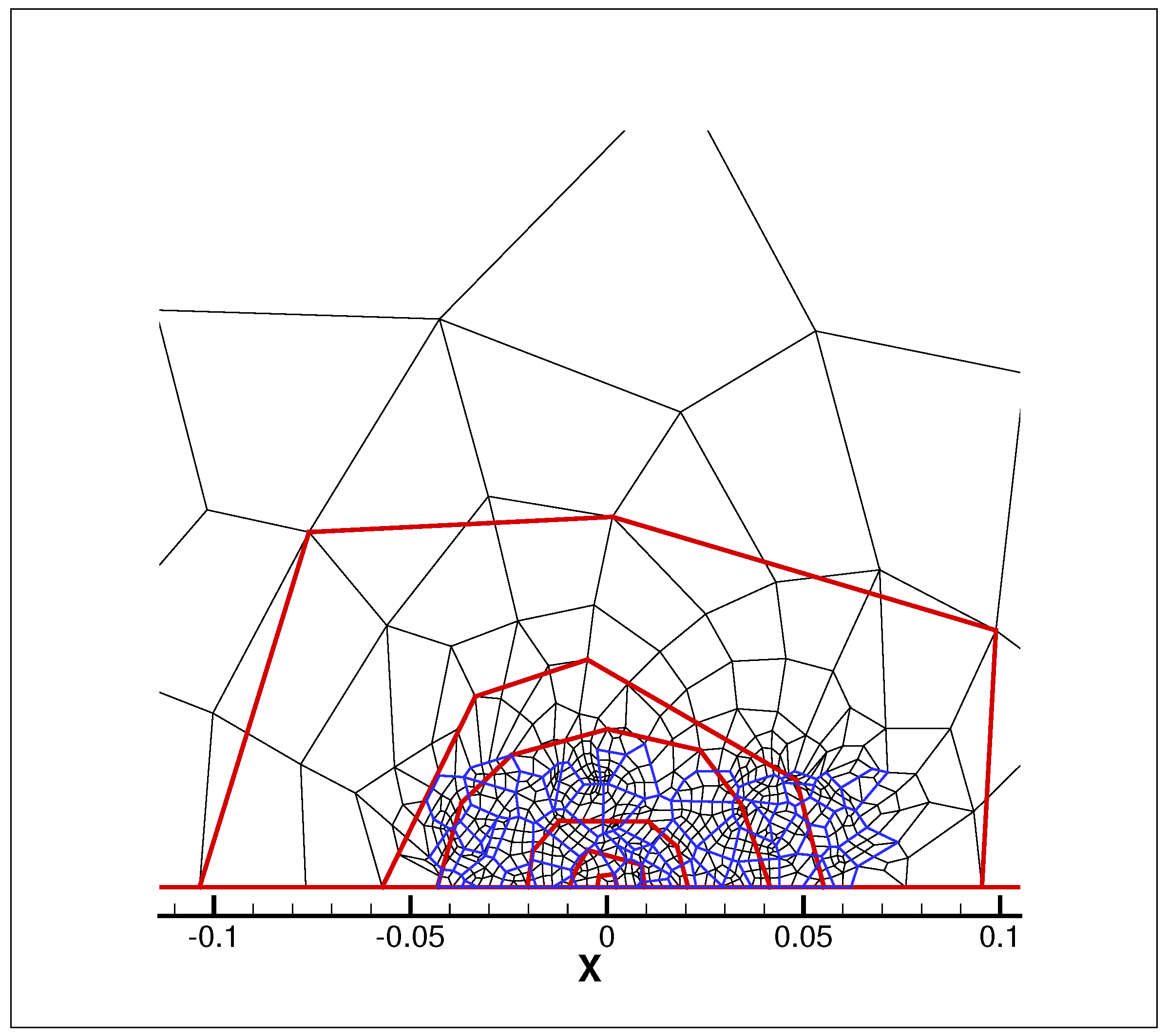
3. Finite Element Algorithm

The equilibrium equation is expressed in the Lagrangian framework as:

$${\nabla }_0·\langle \mathit{P}\rangle +\mathit{f}=\mathbf{0}$$

(13)

where ${\nabla }_0$ is the divergence described in the initial reference configuration ($t=0$) and f denotes the body forces. The polycrystal Piola–Kirchhoff-I stress, $\langle \mathit{P}\rangle$, is defined as:

$$\langle \mathit{P}\rangle =\det \mathit{F}\langle \mathbf{\sigma }\rangle {\mathit{F}}^{-T}$$

(14)

For any kinematically admissible test function $\tilde{\mathit{u}}$, the weak form of the virtual work equation with applied surface traction $\mathbf{\lambda }$ can be written as:

$$\mathcal{G}({\mathit{u}}_{n+1},\tilde{\mathit{u}})\equiv {\int }_{{\mathcal{B}}_0}\langle \mathit{P}\rangle ·{\nabla }_0\tilde{\mathit{u}}dV-{\int }_{\partial {\mathcal{B}}_0}\mathbf{\lambda }·\tilde{\mathit{u}}dA-{\int }_{{\mathcal{B}}_0}\mathit{f}·\tilde{\mathit{u}}dV=0$$

(15)

The Newton–Raphson iterative scheme with a line search procedure is employed to solve the weak form while using a formulation that uses a combination of triangle and quadrilateral elements:

$$\frac{\partial \mathcal{G}({\mathit{u}}_n,\tilde{\mathit{u}})}{\partial {\mathit{u}}_n}\mathrm{\Delta }\mathit{u}={\int }_{{\mathcal{B}}_0}\frac{\partial \langle \mathit{P}\rangle }{\partial \mathit{F}}\frac{\partial \mathit{F}}{\partial {\mathit{u}}_n}·{\nabla }_0\tilde{\mathit{u}}dV\mathrm{\Delta }\mathit{u}=\mathcal{G}({\mathit{u}}_n,\tilde{\mathit{u}})$$

(16)

The linearization process of PK-I stress is given by:

$$\delta \langle \mathit{P}\rangle =\det \mathit{F}\left(\mathrm{tr}\left(\delta \mathit{F}{\mathit{F}}^{-1}\right)\langle \mathbf{\sigma }\rangle -\langle \mathbf{\sigma }\rangle {\left(\delta \mathit{F}{\mathit{F}}^{-1}\right)}^T+\langle \delta \mathbf{\sigma }\rangle \right){\mathit{F}}^{-T}$$

(17)

$\delta \mathbf{\sigma }$ can be expressed as:

$$\begin{array}{cc}\delta \mathbf{\sigma }\hfill & {\displaystyle =\delta \left(-\frac{1}{\det {\mathit{F}}^e}{\mathit{F}}^e\mathit{T}{\left({\mathit{F}}^e\right)}^T\right)}\hfill \\ & {\displaystyle =-tr({{\mathit{F}}^e}^{-1}\delta {\mathit{F}}^e)\mathbf{\sigma }+\delta {\mathit{F}}^e{\left({\mathit{F}}^e\right)}^{-T}\mathbf{\sigma }+\mathbf{\sigma }{\left({\mathit{F}}^e\right)}^{-1}\delta {\left({\mathit{F}}^e\right)}^T+\frac{1}{\det {\mathit{F}}^e}{\mathit{F}}^e\delta \mathit{T}{\left({\mathit{F}}^e\right)}^T}\hfill \end{array}$$

(18)

where $\delta {\mathit{F}}^e$ is obtained as:

$$\delta \left({\mathit{F}}^e\right)=\delta \mathit{F}{\left({\mathit{F}}^p\right)}^{-1}-{\mathit{F}}_{tr}^e\sum _{\beta }sign({\tau }_{tr}^{\beta })\delta \left(\mathrm{\Delta }{\gamma }^{\beta }\right){\mathit{S}}_0^{\beta }$$

(19)

Here, $\delta \mathit{T}$ can be obtained as:

$$\begin{array}{ccc}\delta \mathit{T}\hfill & =& \hfill {\displaystyle {\mathcal{L}}^e\left[\delta {\mathit{E}}_{tr}^e\right]-\frac{1}{2}\sum _{\beta }sign({\tau }_{tr}^{\beta })\delta \left(\mathrm{\Delta }{\gamma }^{\beta }\right){\mathcal{L}}^e\left[{\mathit{B}}^{\beta }\right]}\\ & & {\displaystyle -\sum _{\beta }sign({\tau }_{tr}^{\beta })\mathrm{\Delta }{\gamma }^{\beta }{\mathcal{L}}^e\left[{\mathit{S}}_0^{\beta T}\delta {\mathit{E}}_{tr}^e+\delta {\mathit{E}}_{tr}^e{\mathit{S}}_0^{\beta }\right]}\hfill \end{array}$$

(20)

where, ${\mathit{B}}^{\beta }={({\mathit{S}}_0^{\beta })}^T{\left({\mathit{F}}_{tr}^e\right)}^T{\mathit{F}}_{tr}^e+{\left({\mathit{F}}_{tr}^e\right)}^T{\mathit{F}}_{tr}^e{\mathit{S}}_0^{\beta }$.

This computation of $\delta \mathit{T}$ requires the evaluation of $\delta \left(\mathrm{\Delta }{\gamma }^{\beta }\right)$, obtained by linearization given by:

$$\begin{array}{c}\hfill \delta \left(\mathrm{\Delta }{\gamma }^{\beta }\right)={\left(A^{\alpha \beta }\right)}^{-1}(\delta b^{\alpha }-\delta A^{\alpha \beta }\mathrm{\Delta }{\gamma }^{\beta })\end{array}$$

(21)

$$\begin{array}{c}\hfill \delta b^{\alpha }=\mathrm{sign}\left({\tau }_{tr}^{\alpha }\right){\mathcal{L}}^e\left[\delta {\mathit{E}}_{tr}^e\right]·{\mathit{S}}_0^{\alpha }\end{array}$$

(22)

$$\begin{array}{c}\hfill \delta A^{\alpha \beta }=\mathrm{sign}\left({\tau }_{tr}^{\alpha }\right)\mathrm{sign}\left({\tau }_{tr}^{\beta }\right){\mathit{S}}_0^{\alpha }·{\mathcal{L}}^e\left[{{\mathit{S}}_0^{\beta }}^T\delta {\mathit{E}}_{tr}^e+\delta {\mathit{E}}_{tr}^e{\mathit{S}}_0^{\beta }\right]\end{array}$$

(23)

Using the definition of $\delta {\mathit{E}}_{tr}^e=\mathrm{sym}({{\mathit{F}}^e}_{tr}^T\delta \mathit{F}{{\mathit{F}}^p}^{-1})$, the above set of equations yield an implicit form $\delta \left(\mathrm{\Delta }{\gamma }^{\beta }\right)={\mathit{m}}^{\beta }·\delta \mathit{F}$ for use in Equation (20). Next, $\delta {\mathit{F}}^e$ is obtained from:

$$\begin{array}{c}\hfill \delta \left({\mathit{F}}^e\right)=\delta \mathit{F}{\left({\mathit{F}}^p\right)}^{-1}-{\mathit{F}}_{tr}^e\sum _{\beta }\mathrm{sign}({\tau }_{tr}^{\beta })\delta \left(\mathrm{\Delta }{\gamma }^{\beta }\right){\mathit{S}}_0^{\beta }\end{array}$$

(24)

The average stress and tangent modulus at the macro-scale level are obtained by averaging over the ODF as given in Equation (7). At the micro-scale, the tangent modulus and stress are exactly computed in the elements within individual crystals.

4. Numerical Results

A specific crystal geometry with two slip systems at orientation $-\pi /6$ and $+\pi /6$ is considered [12]. In the 2-D elastic stiffness matrix, $c_{11}=2$ GPa and $c_{12}=c_{44}=1$ GPa. The calculation is done under plane stress conditions. The parameters in the hardening law are taken to be as follows: ${\tau }_0^{\alpha }=10$ MPa, $h_o^{\alpha }=10$ MPa, $s_s^{\alpha }=200$ MPa, $q=1.4$ and $a=2$.

The single edge notch configuration (also called the wedge-opening load (WOL) specimen) is depicted in Figure 3. The calculation is only performed using one half of the model for simplicity. A 5000 N shear force p is applied on the left edge. Specific dimensions are a/w $=0.5$ and h/w$=0.6$, as shown in Figure 1. All of the figures are plotted using non-dimensional variables, $\frac{K_{I}b\sqrt{w}}{p}$ and $r/w$. a is the notch length; w is the width; 2h is the height of the specimen; b is unit thickness; for the plane stress problem, $b=1$ m. The solution leads to a stress singularity at the notch tip. There is a wealth of literature on the use of special elements to capture this crack tip singularity, the most popular of which are the quarter point elements that capture the $1/\sqrt{r}$ dependence of the crack tip singularity in linear elasticity or the $1/r$ dependence in perfect plasticity. However, the singularity of the crack tip solution in crystal plasticity is not known analytically, which makes the design of such elements non-trivial. For simplicity, conventional finite elements (the combination of three-noded triangular and four-noded rectangular elements) are employed in these simulations. Meaningful values of crack tip stress intensity factors can be obtained using this approach with the computational procedures demonstrated in Chan (1970) [10].

We only consider the Mode I crack in our paper. The stress intensity factor calculation follows Chan’s paper [10]. Stress intensity $K_I^{*}$ from the displacement-based method:

$$K_I^{*}={\left[\frac{2\pi }{r}\right]}^{\frac{1}{2}}\frac{G{v}^{*}}{f(\theta ,\nu )}$$

(25)

$f(\theta ,\nu )=sin(\frac{\theta }{2})\left[2-2\nu -{cos}^2\frac{\theta }{2}\right]$, $v^{*}$ is the computed nodal displacement in the y direction. The $K_I^{*}$ is obtained by substituting a calculated nodal point displacement $v^{*}$ at point $(r,\theta )$. If the $v^{*}$ were the exact theoretical value, then the value of $K_I^{*}$ will also be exact. The above equation is for the plane strain situation; for plane stress cases, just replace $\nu$ with $\nu /(1+\nu )$ for $f(\theta ,\nu )$.

The stress intensity factor $K_I^{*}$ from the stress-based method was also used for comparison:

$$K_I^{*}=\frac{{\left(2\pi r\right)}^{\frac{1}{2}}{\sigma }_{yy}^{*}(r,\theta )}{f_{yy}\left(\theta \right)}$$

(26)

$f_{yy}\left(\theta \right)=cos(\theta /2)\left[1+sin(\theta /2)sin(3\theta /2)\right]$. This theoretical result is obtained from the collocation method described in [13].

The J integral is calculated as:

$$J={\int }_{\mathsf{\Gamma }}\left(Wdy-\mathit{T}·\frac{\partial \mathit{u}}{\partial x}ds\right)$$

(27)

The $\mathsf{\Gamma }$ is an arbitrary curve surrounding the crack tip. W is the strain energy density, while T is the traction vector defined by the out normal along $\mathsf{\Gamma }$, $T_i={\sigma }_{ij}{n}_j$, and u is the displacement vector. The integral is evaluated counterclockwise around the crack tip. The reported J value is twice the half plane’s J value. Strain energy density W is found from PK-I stress and deformation gradient F, $W={\int }_{{\mathsf{\Omega }}_0}\mathit{P}:\delta \mathit{F}dV$. The shear force on the left boundary of the model is applied over 20 steps to get the value of p.

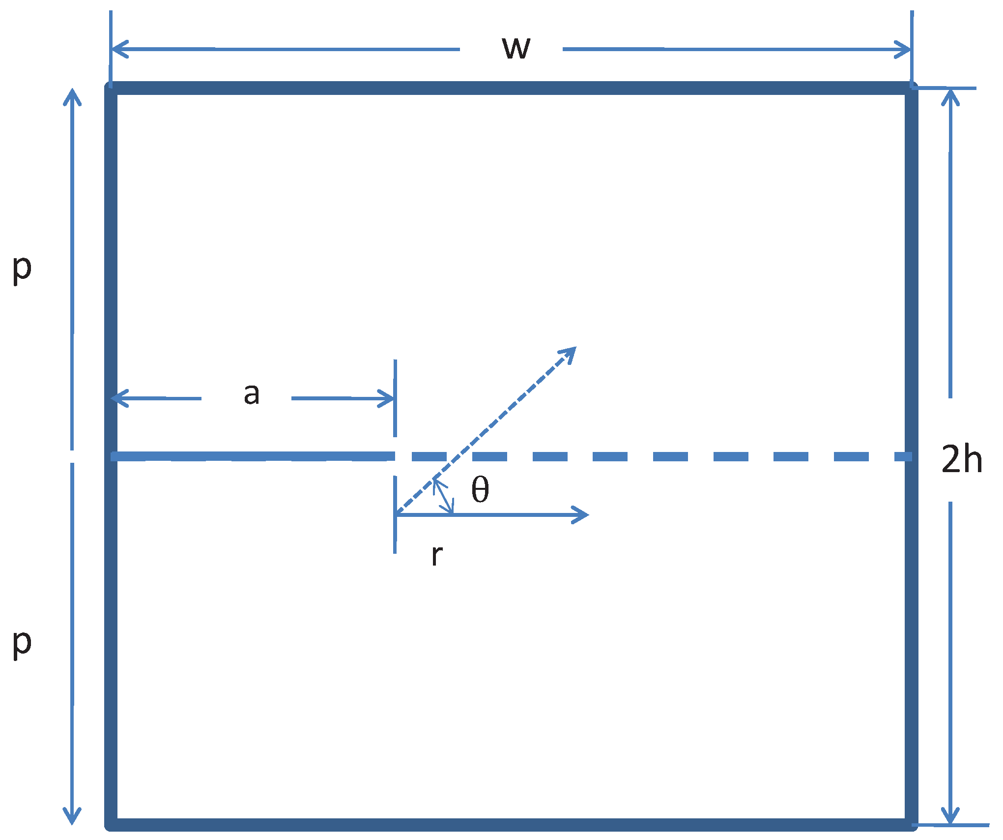
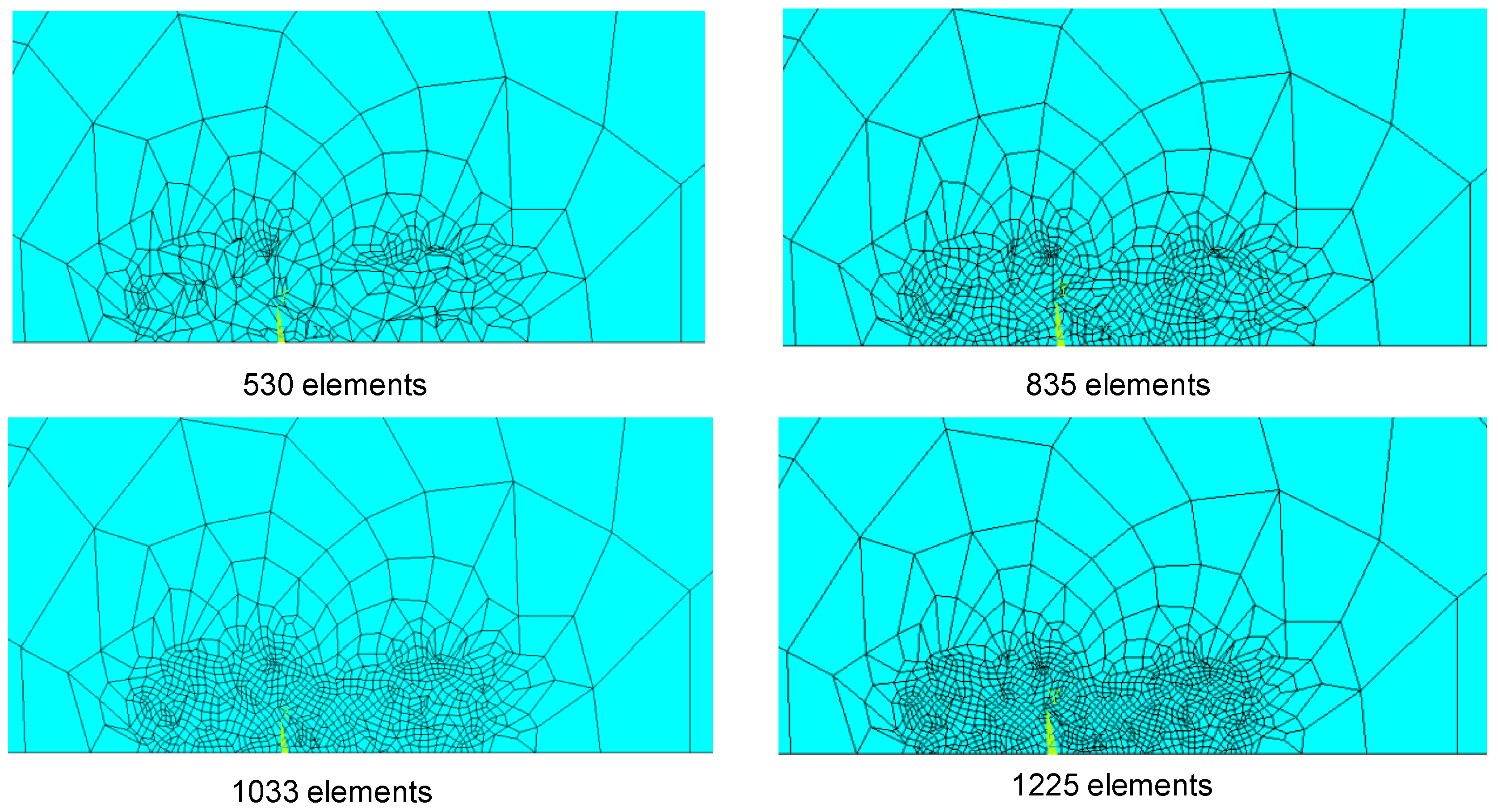
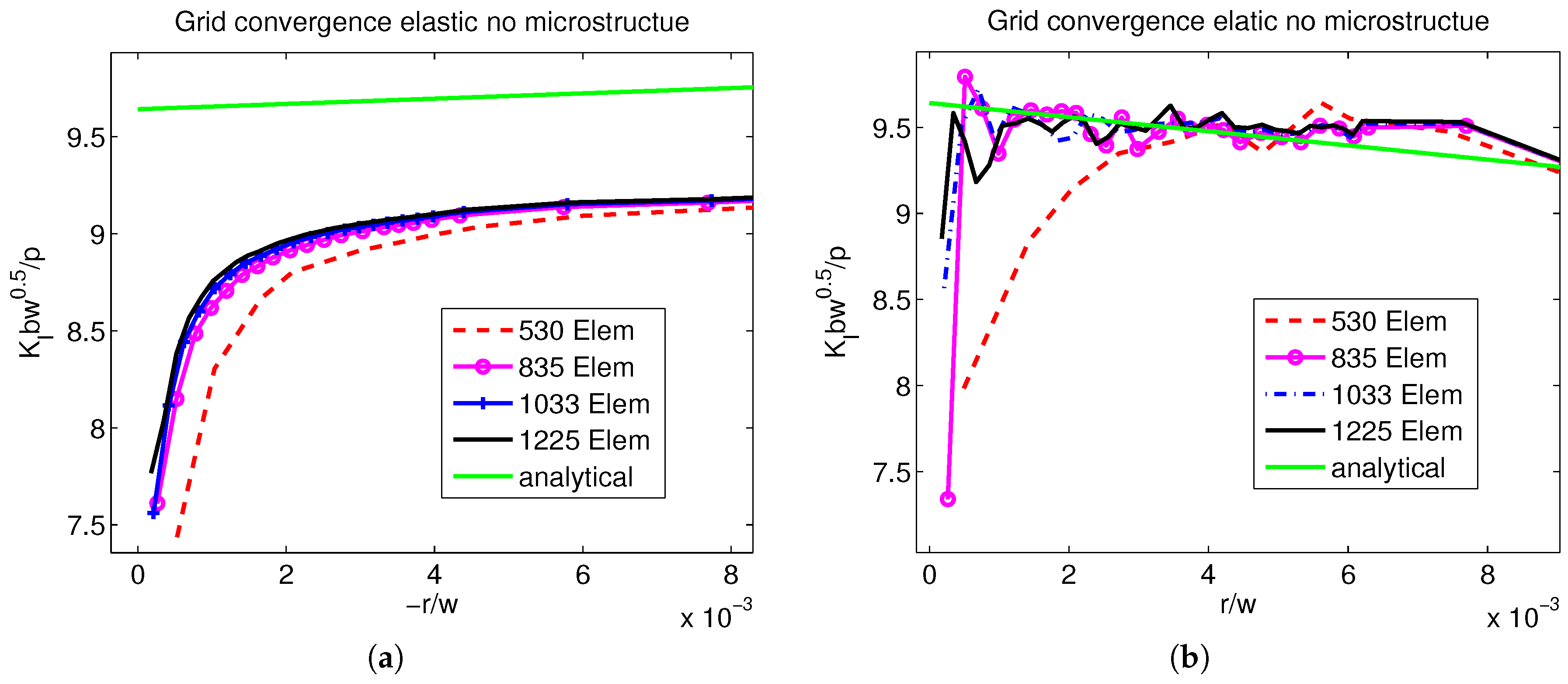
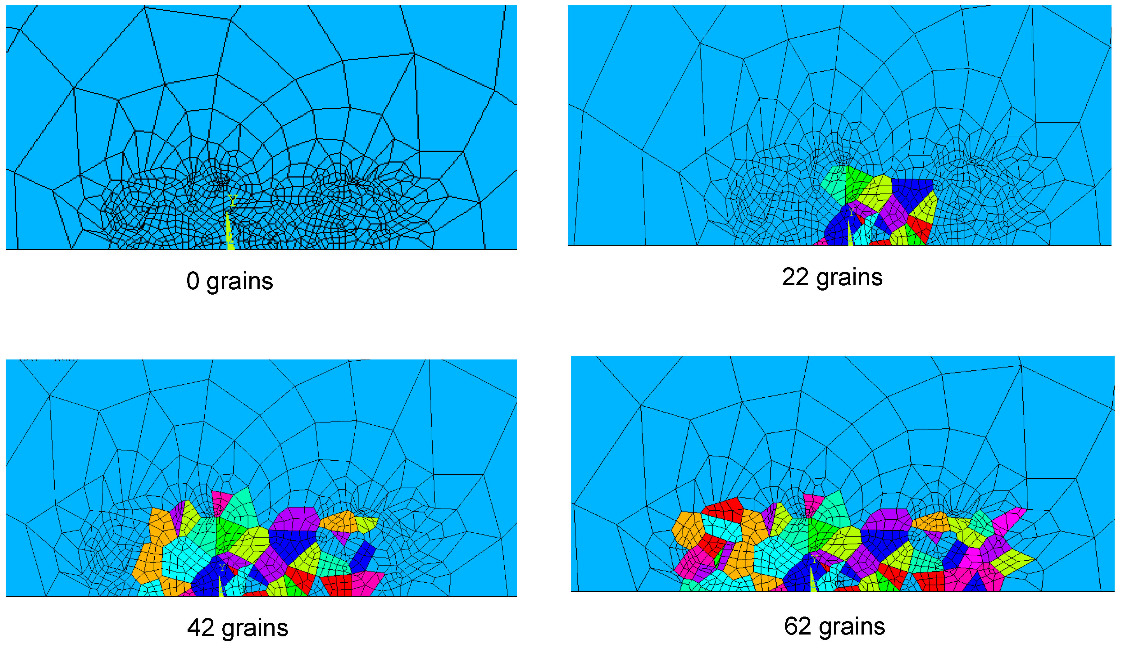
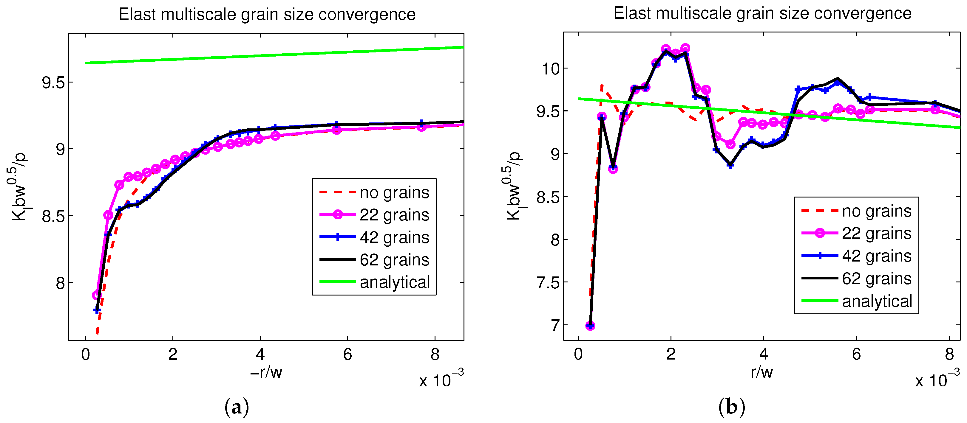
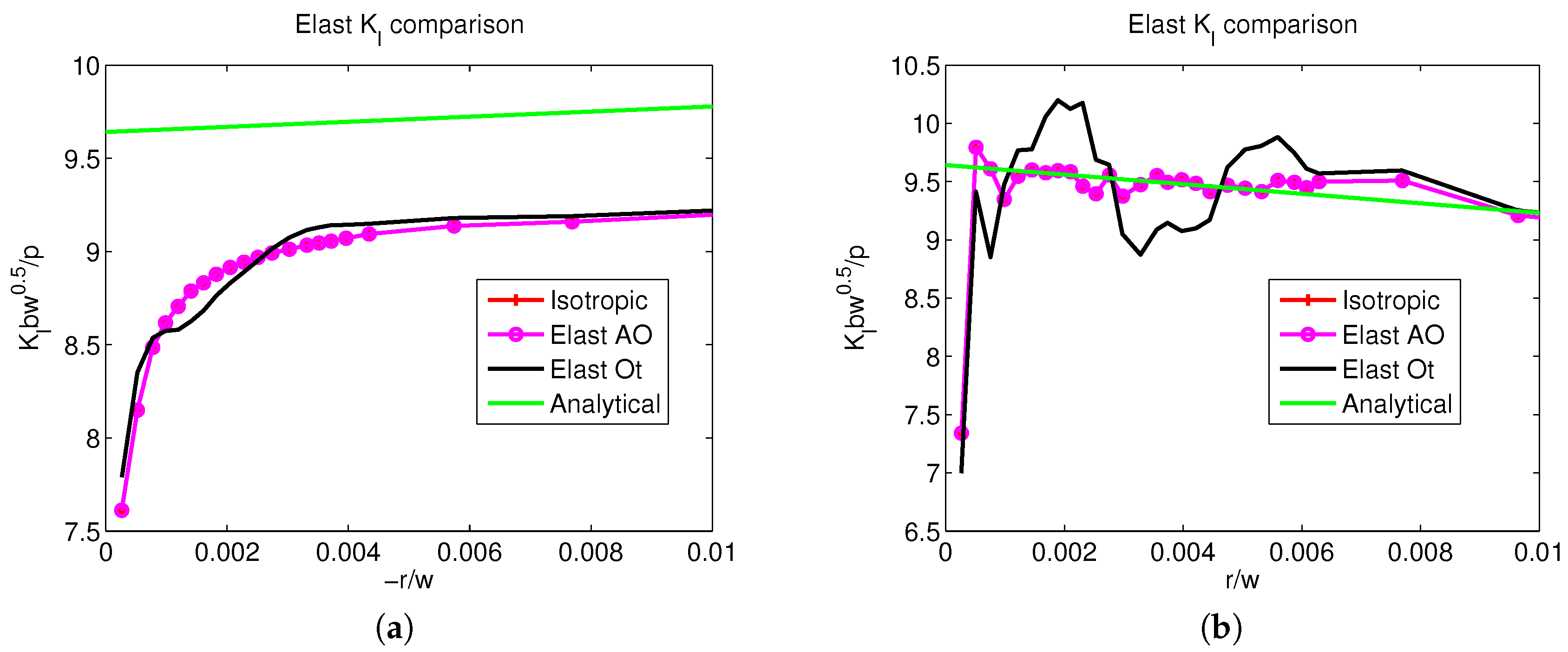
4.1. Linear Elastic Simulations

The first few tests were performed by setting the plastic shearing strain to zero $\mathrm{\Delta }\gamma =0$ which leads to a fully-elastic model. In the convergence results shown below, the displacement on the crack surface ($\theta =\pi$) and stress ${\sigma }_{yy}$ on the $\theta =0$ plane (away from the crack in the positive xdirection) are shown. First, a convergence test is performed on different meshes by progressively refining the element size in the microstructure; see Figure 4. In this simulation, a fully-isotropic model is employed without any microstructure. The test shows good convergence with the increasing number of elements, as shown in Figure 5, and the results are similar to those reported in the finite element model of [10]. The analytical result is from [13].

A similar convergence test was performed by altering the number of grains in the vicinity of the crack tip (and 835 elements in each case; see Figure 6). The zero grain case corresponds to the isotropic elastic case (with a fully-random ODF). This corresponds to an isotropic stiffness matrix with $c_{11}=2.25\mathrm{GPa}$, $c_{12}=0.75\mathrm{GPa}$ and $c_{44}=0.75\mathrm{GPa}$. The grain convergence study allows one to choose the size of the critical region that needs to be modeled using microstructural grids. From the results shown in Figure 7, there is a trend towards convergence with the increasing number of grains. As the number of grains increases from 42 to 62, little additional accuracy is realized. This implies that a 42-grain case is sufficient to address this particular problem. Beyond this point, the ODF model may be employed. Further, a quick comparison of the zero grain case (isotropic solution) with the 62 grain case result in Figure 7 clearly depicts the role of the microstructure in determining the stress concentration at the crack tip. When $r/w$ is smaller than $6\times {10}^{-3}$, stress concentrations deviate from the isotropic case. While $r/w$ is larger than $6\times {10}^{-3}$, the microstructure does not play a significant role, and the result converges back to the isotropic solution.

Subsequently, three models are compared: (i) a model with isotropic properties; (ii) a model with every element having an underlying ODF (called an ‘all-ODF’ model) with no explicit microstructure; (iii) a multiscale model with explicitly-modeled crystal orientations (called ‘Elastic-Ot’model) near the crack tip and ODF representation at the far field. The detailed comparison between these models is shown in Figure 8. Firstly, the all-ODF model (with the initial random ODF) has the exact same result as the isotropic elastic model as expected. The model with the explicit microstructure has larger variations in stress concentration near the crack tip. Figure 9 additionally depicts the resolved shear stress in the two slip systems for the elastic model as overlaid on the grains showing significant variability in stresses from grain to grain, stressing the need for a microstructure model at critical regions.

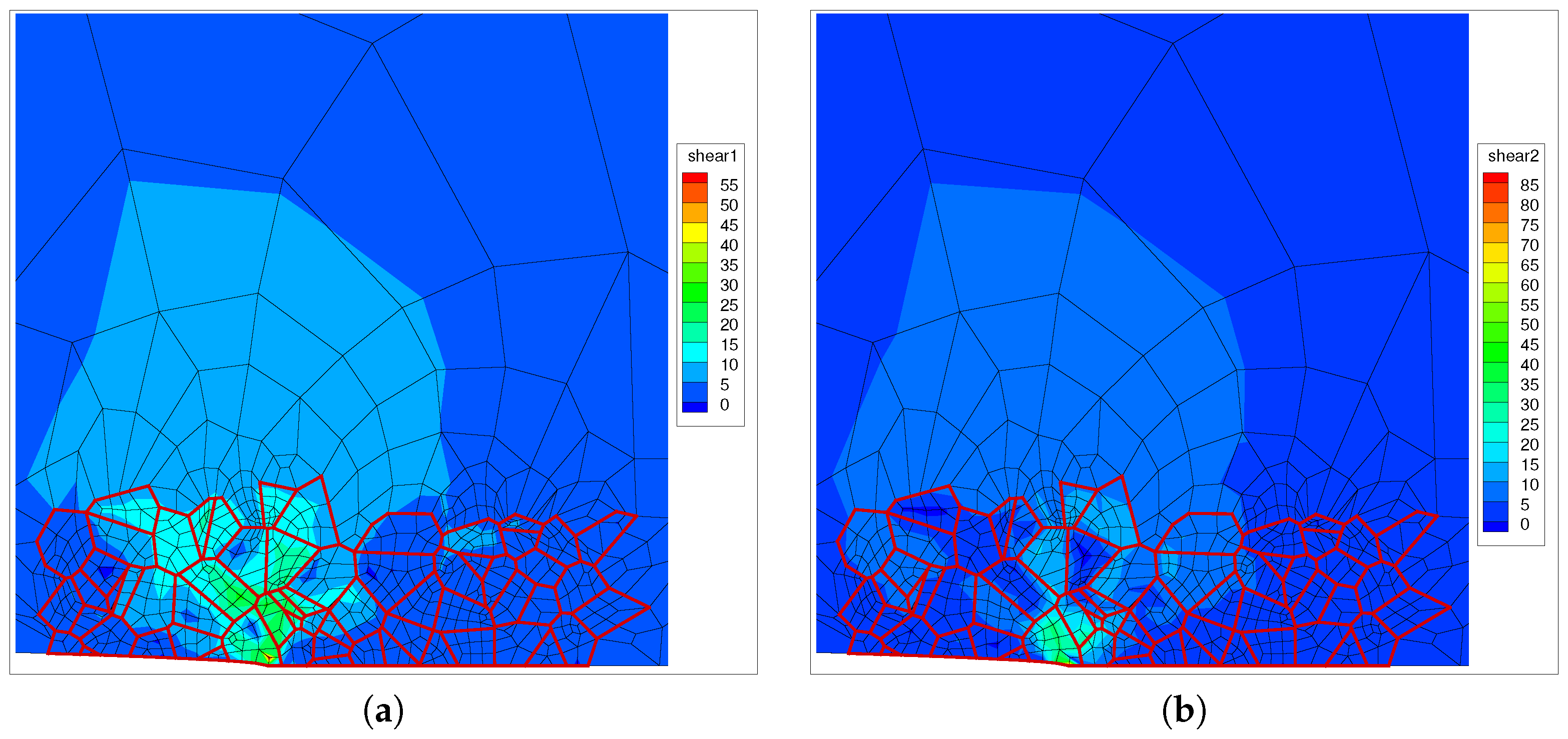
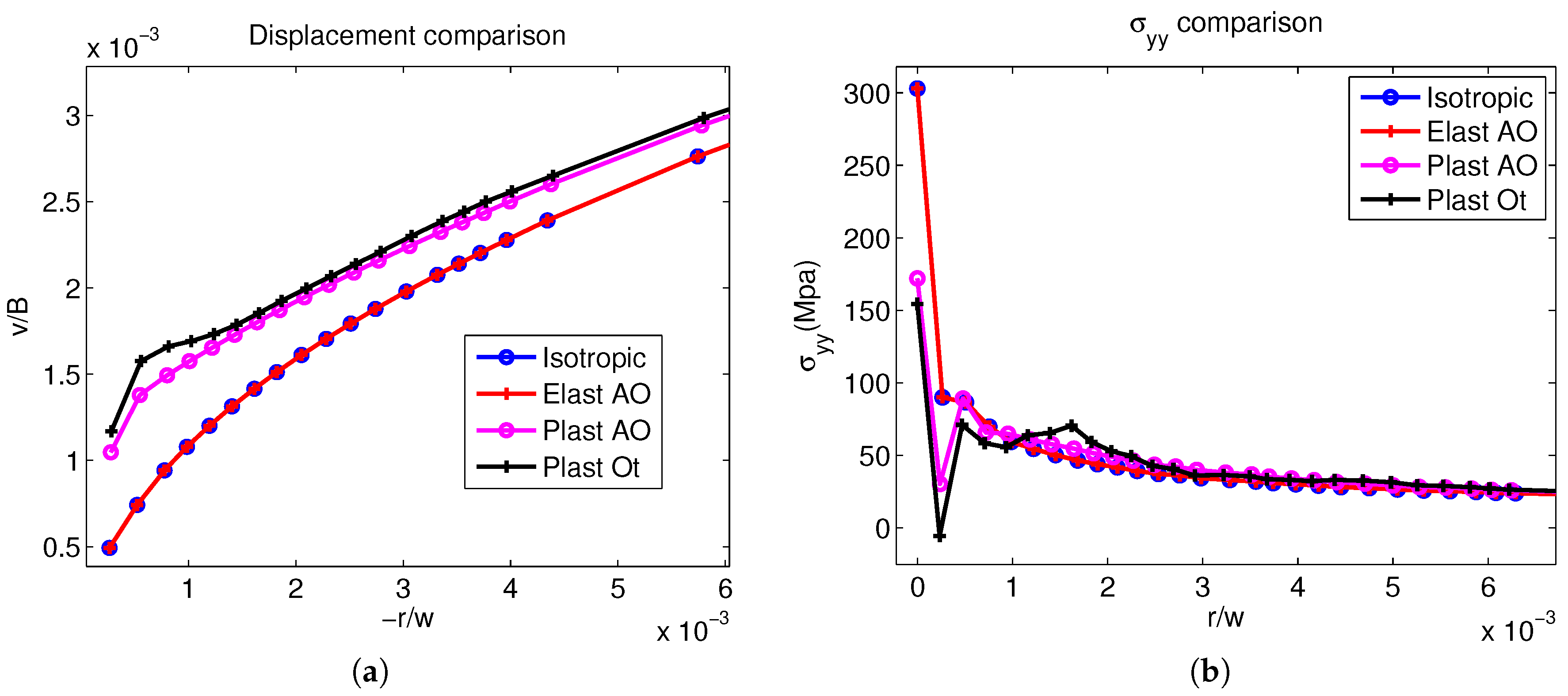
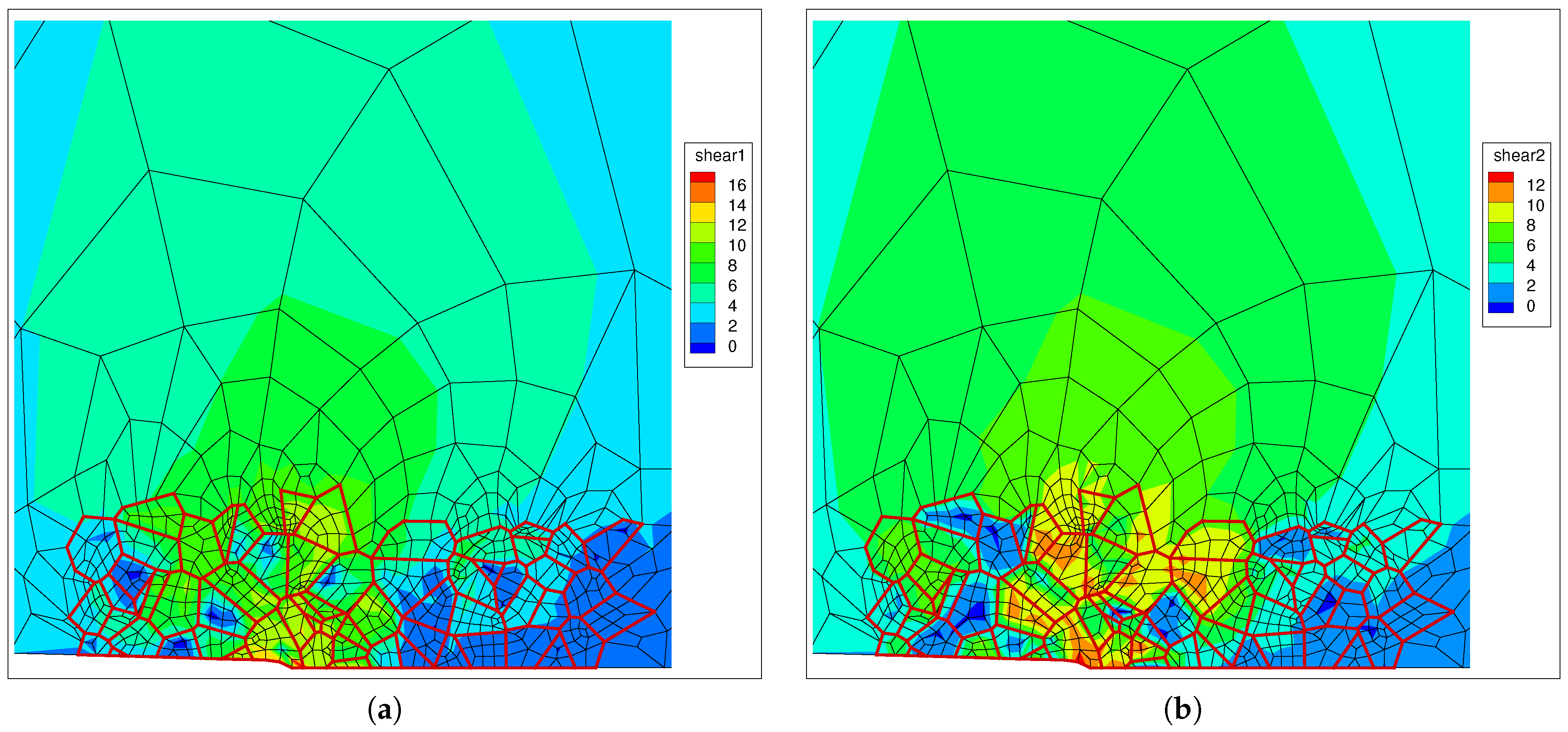
4.2. Elasto-Plastic Simulations

In subsequent simulations, notch tip plasticity is turned on. All test cases are based on meshes with 835 elements and 62 grains cover the notch tip area. The inclusion of notch tip plasticity leads to a larger displacement at the crack tip (and also smaller stress near the crack tip). This is seen in Figure 10 where the displacements and stresses are directly compared to the elastic case. These results are subsequently shown in terms of the non-dimensional stress intensity factor in Figure 11. Note that on the $\theta =\pi$ plane, the stress intensity factor Equation (25) as computed from the elasticity-based formula will be larger in the plastic case due to larger displacements. On the other hand, the smaller stress ${\sigma }_{yy}$ on the $\theta =0$ plane will lead to a smaller ${\mathit{K}}_I$ value based on Equation (26). These are simply artifacts of using an elasticity-based analytical solution to calculate the stress intensity factor. Due to the larger displacement and smaller stresses around crack tips, elasto-plastic results show altogether different ${\mathit{K}}_I$ trends when compared to the fully-elastic case in Figure 8.

Next, comparing an all-ODF model with plasticity (zero grains) and one with the microstructure explicitly modeled, the differences between these two cases (shown in Figure 11) are much more pronounced than the fully-elastic case (that did a similar comparison between no grains and the 62-grain case; see Figure 7). The inclusion of the microstructure significantly affects the calculated stress intensity factor, which is important during the assessment of safety factors during component design. Figure 12a,b additionally depicts the resolved shear stress in the two slip systems for the elasto-plastic model as overlaid on the grains. This again shows significant variability in stresses from grain to grain, but stresses are smaller than the fully-elastic case shown in Figure 9 as expected. As addressed in McMeeking [14] and Rice and Johnson [15], the crack tip plastic blunting can also be explained by exploiting the crack tip opening stresses. However, instead of using the analytical method, we will employ the J-integral approach next to more reliably compare the elastic and elastoplastic cases.

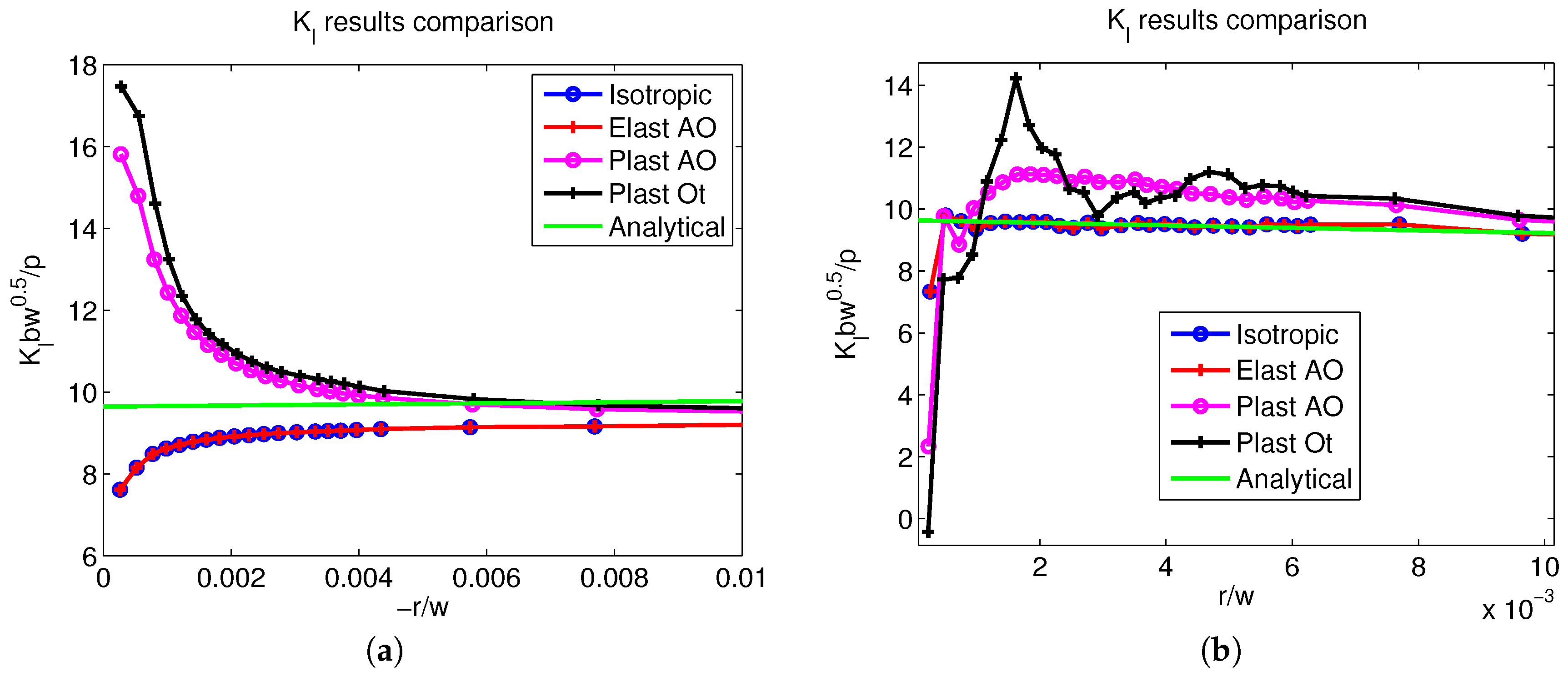
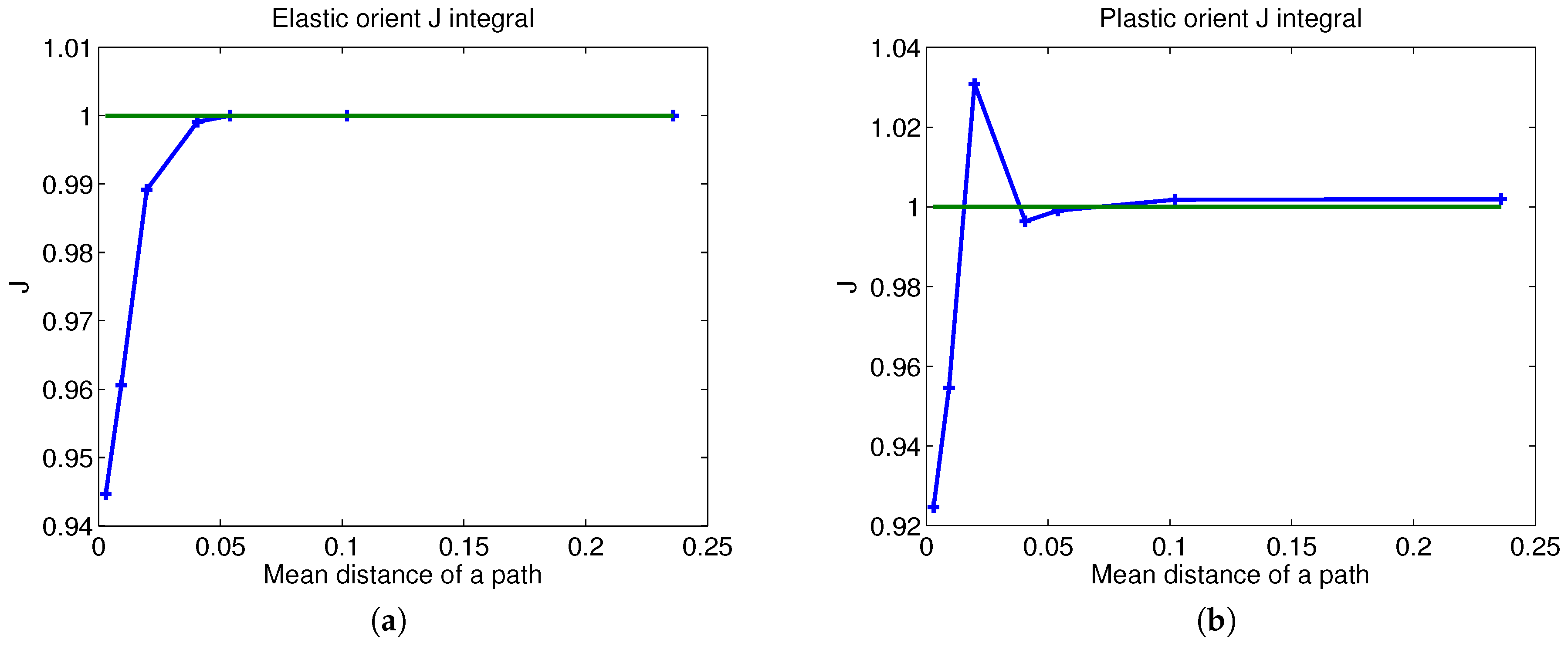
4.3. J Integral Calculation

In order to numerically evaluate the J integral, several loops are drawn around the crack tip as shown in Figure 13. The inner-most curve is within only one grain, while the outmost curve circumscribes the entire microstructure. The results of the J integral calculations are shown in Figure 14. The J integrals of multiscale models (with microstructure) are normalized with respect to that of a fully-homogenized model (with no grains). The x-coordinate is the mean distance values of points on different integral curves. Figure 14a shows the J values of the elastic model. The elastic model with the microstructure has lower J values at the crack tip, but converges to a homogenized model at the far field. Figure 14b shows the J integral of the elastoplastic model. This model also converges to the homogenized model result at the far field; however, the near field J values oscillate because of the microstructural influence. This trend is similar to those shown in Figure 8 and Figure 11 in that the model with the microstructure has more prominent oscillation of stress intensities around the crack tip in the case of an elastoplastic model.

In the elastic case, the ODF does not evolve with deformation. However, in the elastoplastic case, the texture evolves close to the crack tip with the specimen deformation. Texture evolves in the region modeled explicitly with the microstructure, at the same time, and Figure 15 shows the case of ODF evolution in the homogenized region.

5. Conclusions

The proposed multi-scale model combines the computational efficiency of statistical approaches with the accuracy of CPFEat critical regions. The approach can provide detailed stress and displacement results around critical regions such as crack tips and localized loads (e.g., indentation tests) while also providing good estimates of far field stresses. As an illustrative example, we applied the multiscaling method to compute the stress intensity factor ${\mathit{K}}_I$ around the crack tip in a wedge-opening load specimen [10]. The approach was verified with an analytical solution within linear elasticity and has been extended to allow the modeling of crack tip plasticity. We are currently extending this framework to allow modeling of arbitrary crack paths at critical regions within the multiscale approach.

References

1. Allison, J.; Backman, D.; Christodoulou, L. Integrated Computational Materials Engineering: A New Paradigm for the Global Materials Profession. J. Miner. Met. Mater. Soc. 2006, 58, 25–27. [Google Scholar] [CrossRef]
2. Sundararaghavan, V.; Zabaras, N. Design of microstructure-sensitive properties in elasto-viscoplastic polycrystals using multi-scale homogenization. Int. J. Plast. 2006, 22, 1799–1824. [Google Scholar] [CrossRef]
3. Sundararaghavan, V.; Zabaras, N. A multi-length scale continuum sensitivity analysis for the control of texture-dependent properties in deformation processing. Int. J. Plast. 2008, 24, 1581–1605. [Google Scholar] [CrossRef]
4. Miller, R.; Tadmor, E.B.; Phillips, R.; Ortiz, M. Quasicontinuum simulation of fracture at the atomic scale. Model. Simul. Mater. Sci. Eng. 1998, 6, 607–638. [Google Scholar] [CrossRef]
5. Dunne, F.P.E.; Wilkinson, A.J.; Allen, R. Experimental and computational studies of low cycle fatigue crack nucleation in a polycrystal. Int. J. Plast. 2007, 23, 273–295. [Google Scholar] [CrossRef]
6. Clement, A. Prediction of deformation texture using a physical principle of conservation. Mater. Sci. Eng. 1982, 55, 203–210. [Google Scholar] [CrossRef]
7. Sundararaghavan, V.; Kumar, A. Probabilistic modeling of microstructure evolution using finite element representation of statistical correlation functions. Int. J. Plast. 2012, 30–31, 62–80. [Google Scholar] [CrossRef]
8. Kumar, A.; Dawson, P.R. The simulation of texture evolution using finite elements over orientation space. I. Development. Comput. Methods Appl. Mech. Eng. 1996, 130, 227–246. [Google Scholar] [CrossRef]
9. Kumar, A.; Dawson, P.R. The simulation of texture evolution using finite elements over orientation space. II. Application to planar crystals. Comput. Methods Appl. Mech. Eng. 1996, 130, 247–261. [Google Scholar] [CrossRef]
10. Chan, S.K.; Tuba, I.S.; Wilson, W.K. On the finite element method in linear fracture mechanics. Eng. Fract. Mech. 1970, 2, 1–17. [Google Scholar] [CrossRef]
11. Anand, L.; Kothari, M. A computational procedure for rate-independent crystal plasticity. J. Mech. Phys. Solids 1966, 44, 525–558. [Google Scholar] [CrossRef]
12. Sun, S.; Sundararaghavan, V. A probabilistic crystal plasticity model for modeling grain shape effects based on slip geometry. Acta Mater. 2012, 60, 5233–5244. [Google Scholar] [CrossRef]
13. Gross, B.; Srawley, J.E.; Brown, W.F. Stress-Intensity Factors for a Single-Edge-Notch Tension Specimen by Boundary Collocation of a Stress Function; NASA Technical Report (No. NASA-TN-D-2395); National Aeronautics and Space Administration: Washington, DC, USA, 1964. [Google Scholar]
14. McMeeking, R.M. Finite deformation analysis of crack-tip opening in elastic-plastic materials and implications for fracture. J. Mech. Phys. Solids 1977, 25, 357–381. [Google Scholar] [CrossRef]
15. Rice, J.R. The role of large crack tip geometry changes in plane strain fracture. In Inelastic Behavior of Solids; Kanninen, M.F., Ed.; McGraw-Hill: New York, NY, USA, 1970; pp. 641–672. [Google Scholar]
Figure 1. The configuration of the multi-scale model. The model is divided into two scales. The microscale is the critical areas containing crystals with orientations. The macroscale element has an orientation distribution function (ODF) in each integration point representing hundreds to thousands of crystals.
Metals 07 00345 g001
Figure 2. Probability update scheme in finite element (FE) space: During deformation, the nodal points (g) of the FE mesh are moved to reflect the reorientation ( Δ g ) of crystals. The new ODF is obtained using Equation (4), which ensures that the normalization constraint (Equation (2)) is met in the reoriented mesh.
Metals 07 00345 g002
Figure 3. The single-edge notch configuration with width w, height 2h and shear force p is applied on the left edge. Only the upper half is modeled.
Metals 07 00345 g003
Figure 4. Grids of 530, 835, 1033 and 1225 elements discretizing 62 grains.
Metals 07 00345 g004
Figure 5. Grid convergence test with 530 elements, 835 elements, 1033 elements and 1225 elements of 62 grains on the elastic all-ODF model. The analytical line is from the collocation method. (a) Non-dimensional K I from the displacement method; (b) non-dimensional K I from the stress method. Both results show convergence at 835 elements.
Metals 07 00345 g005
Figure 6. Grids with increasing number of grains near the crack tip (22, 42 and 62 grains) with 835 elements. Different numbers of grains are used to test the critical area that needs to be covered by crystals.
Metals 07 00345 g006
Figure 7. Size convergence test with 0, 22, 42 and 62 grains. (a) Non-dimensional K I from the displacement method; (b) non-dimensional K I from the stress method. The results show that convergence can be achieved by more than 42 grains.
Metals 07 00345 g007
Figure 8. Normalized stress intensity factor plotted as a function of the distance from the crack tip for different models. (a) displacement-based method and (b) stress-based method.
Metals 07 00345 g008
Figure 9. Resolved shear stress (all units in MPa) results in (a) slip system 1 and (b) slip system 2, for the multiscale model with orientations. The maximum shear stresses reach as high as 85 MPa.
Metals 07 00345 g009
Figure 10. Comparison between elastic and elastoplastic models. (a) y-displacements; (b) σ y y . Inclusion of the microstructure leads to larger variability in values.
Metals 07 00345 g010
Figure 11. Comparison of stress intensity factors for elastic and elastoplastic models when using an elasticity-based analytical solution. K I calculated from plastic models returns a different trend when compared to elastic models. (a) displacement-based method and (b) stress-based method.
Metals 07 00345 g011
Figure 12. Resolved shear stress (all units in MPa) results in two slip systems for the plastic model with the explicitly-modeled microstructure.
Metals 07 00345 g012
Figure 13. J integral curves around the crack tip: the red lines are curves; blue lines are crystals; and black ones are FE elements. The innermost curve is only within one crystal. Other curves cover larger areas than the first one. Each edge of the curve is divided into 10 parts. This means that if the curve has five edges, and there are 50 points to be integrated for the J integral. All distances are in mm.
Metals 07 00345 g013
Figure 14. J integral comparison. (a) Normalized J values of the elastic model with the microstructure. The elastic model with the microstructure has lower J values at first, but converges to the isotropic model at the far field. (b) Normalized J values of the plastic model with the microstructure. The near field plastic J values oscillate due to the influence of the microstructure.
Metals 07 00345 g014
Figure 15. The final texture returned by in the plastic model at the macro-scale elements. The final ODFs at different integration points are different from each other; while for the elastic result, the final ODFs at differentintegration points are the same.
Metals 07 00345 g015