Algorithm for Improvement of a Wrongly Adverted Filling Profile in Injection Flow

Abstract

As Eulerian description is generally used for the simulation of filling flow problems in the powder injection molding process, and the governing equation of the filling state takes the form of an advection equation, the distortion can be easily produced when dealing with the filling process in complex cavities, such as the similar channels in shapes of $\perp$ and L, inside which the phenomena of opposite joining and bypass are involved. In order to improve the precision, causes of the unrealistic results were analyzed in the present paper. A notion similar to the upwind method was introduced and a corresponding correction method was proposed to settle this problem. Based on the efficient explicit algorithm for PIM simulation, and by means of systematic operation to modify the fluid velocity field, the untrue impact of air flow, represented by the velocity field in front of the filling fronts, can be weakened. Then, the advection of the filling state can be mainly affected by the flow field behind the filling front. The simulation results show that the correction algorithm can effectively inhibit the distortion. The simulation of the filling processes in the complex cavities, inside which the flow directions will be subject to the sudden changes, can be realized correctly.

1. Introduction

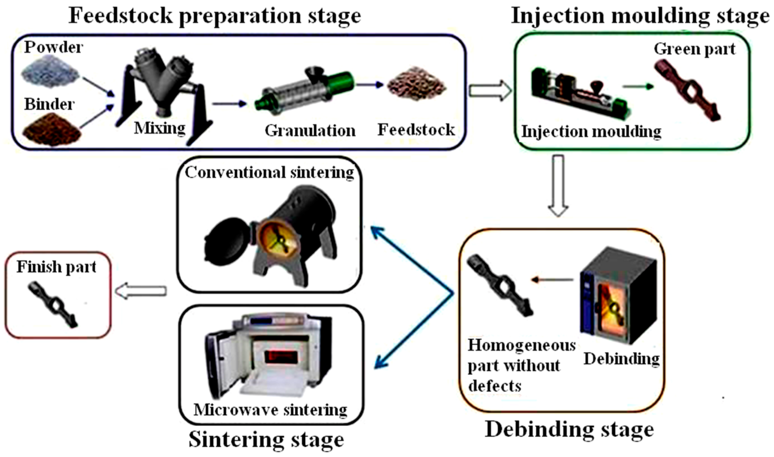
The PIM (powder injection molding) process is somewhat similar to plastic injection molding. It combines the well-known polymer injection molding and powder metallurgy techniques. It consists of the following stages: feedstock preparation, injection molding, debinding of the green parts, and sintering of the brown parts [1]. The PIM process is stated in Figure 1.

With the development of injection molding techniques, the shape of the parts is increasingly complex [3]. Due to the constraints in physical experiments and the availability of measurements for micro-scale factors, the accurate numerical simulation becomes more and more important in designing and manufacturing [4]. Some studies on 3D simulation of the polymer injection molding can also be retrieved in recent years [5,6]. 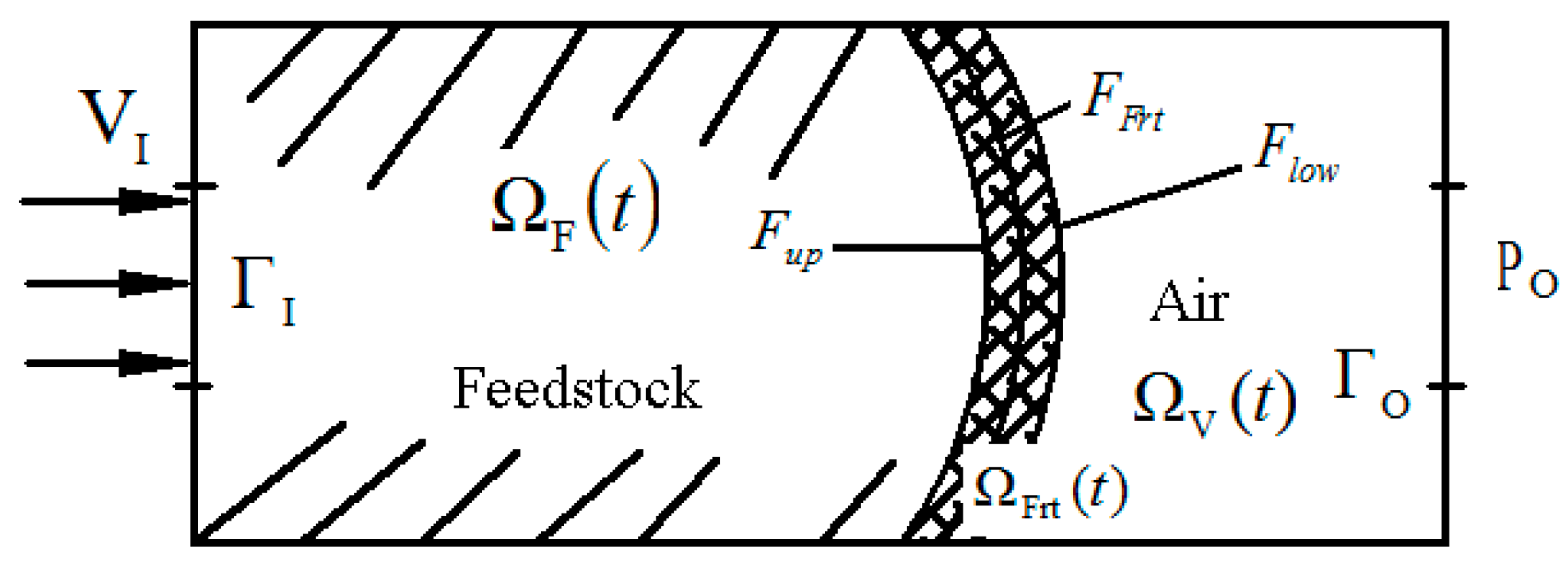In general, Eulerian description is used for simulation of the filling flow problems [7,8]. The mold cavity is assumed occupied by two different flow substances, viscous feedstock in the filled portion and air in the remained void part. 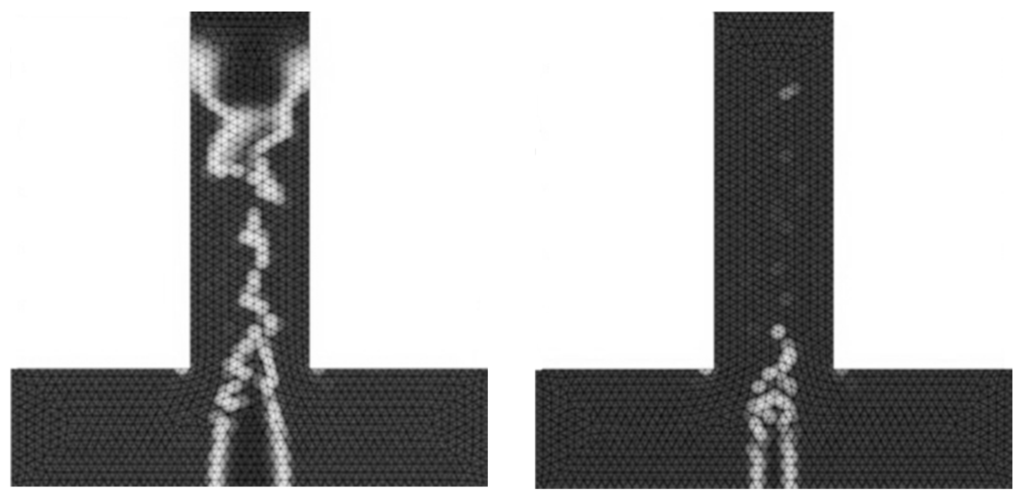A filling state variable F(x,t) is used to describe the evolution of the filling process. The evolution of the filling state is governed by the velocity field in the whole mold cavity. In most cases, the filling flow direction does not change dramatically. The velocity field in the void portion closest to the filling front is similar to that of the feedstock behind the filling front. So, according to the traditional mechanical model of the injection filling process, it will often result in a good and real simulation. 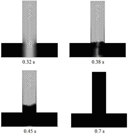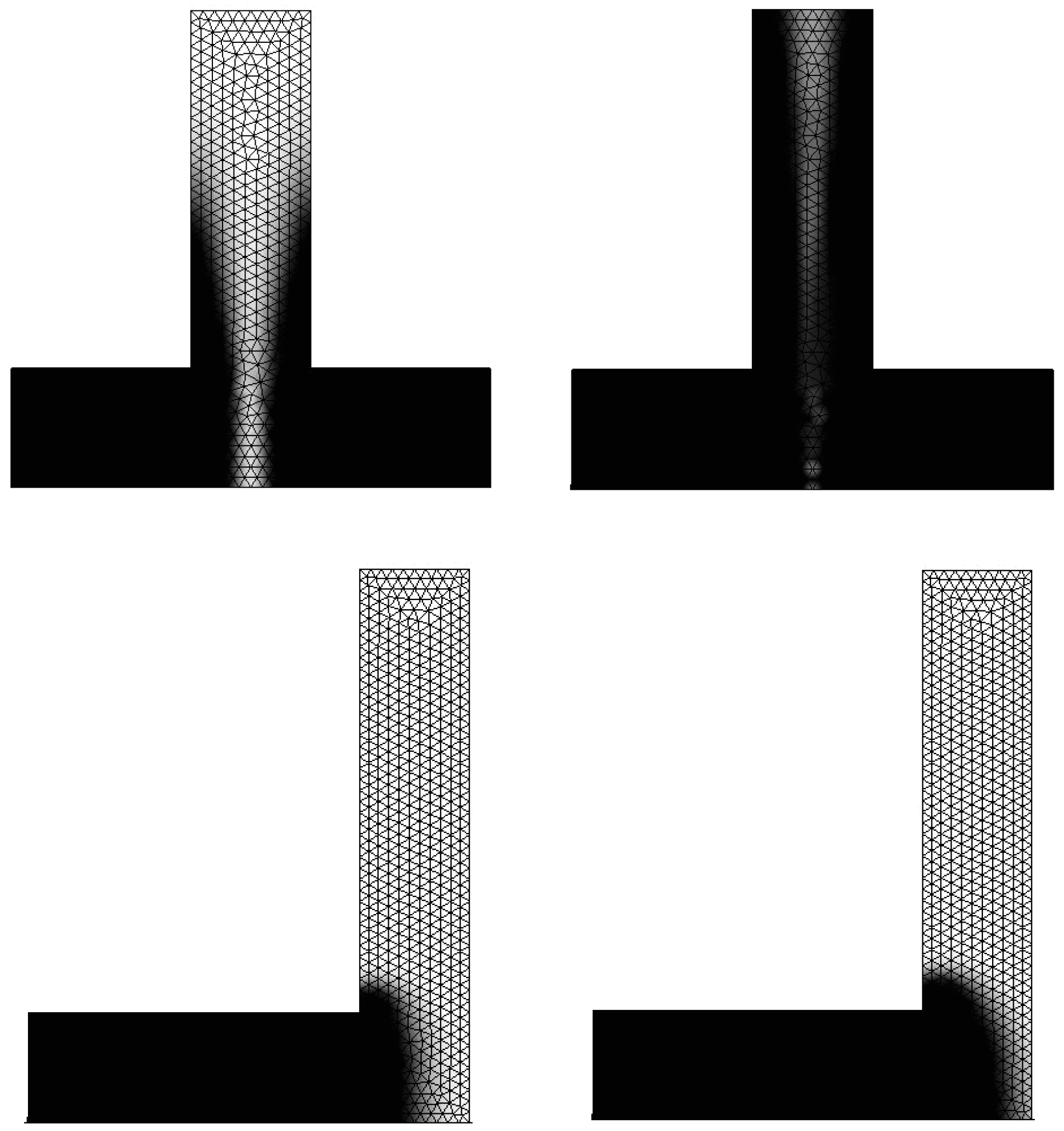However for some cases, it is observed that the filling patterns predicted by simulation are not the realistic ones, especially when the phenomena of opposite joining and bypass are involved, such as channels in shapes like $\perp$ and L. The flow directions will be subject to the sudden changes when filling in these channels. Then, the untrue results may be produced, as shown in Figure 2.

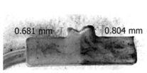
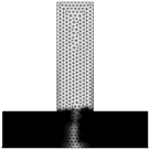
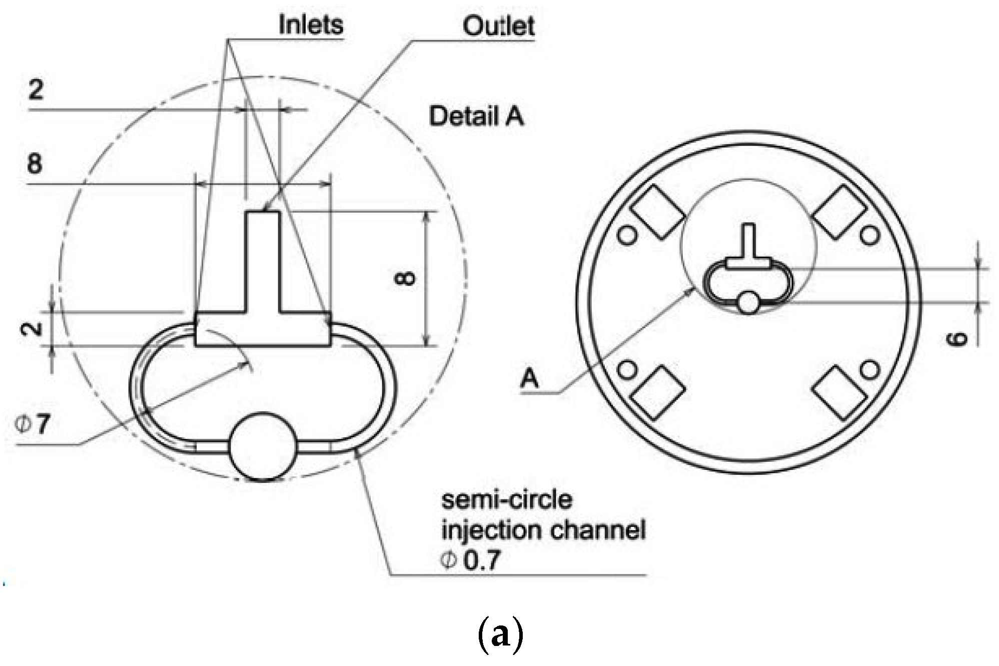
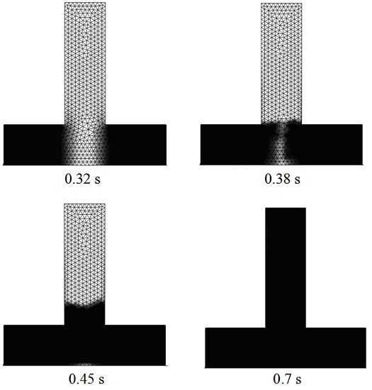
For the case of channel in shape $\perp$, the feedstock is injected from two inlets on opposite sides of the cavity. The same injected velocity was loaded in both inlets. The two different filling fronts with the same speed should independently progress in the mold cavities, and then meet to each other to reach a common outlet. 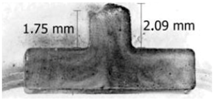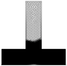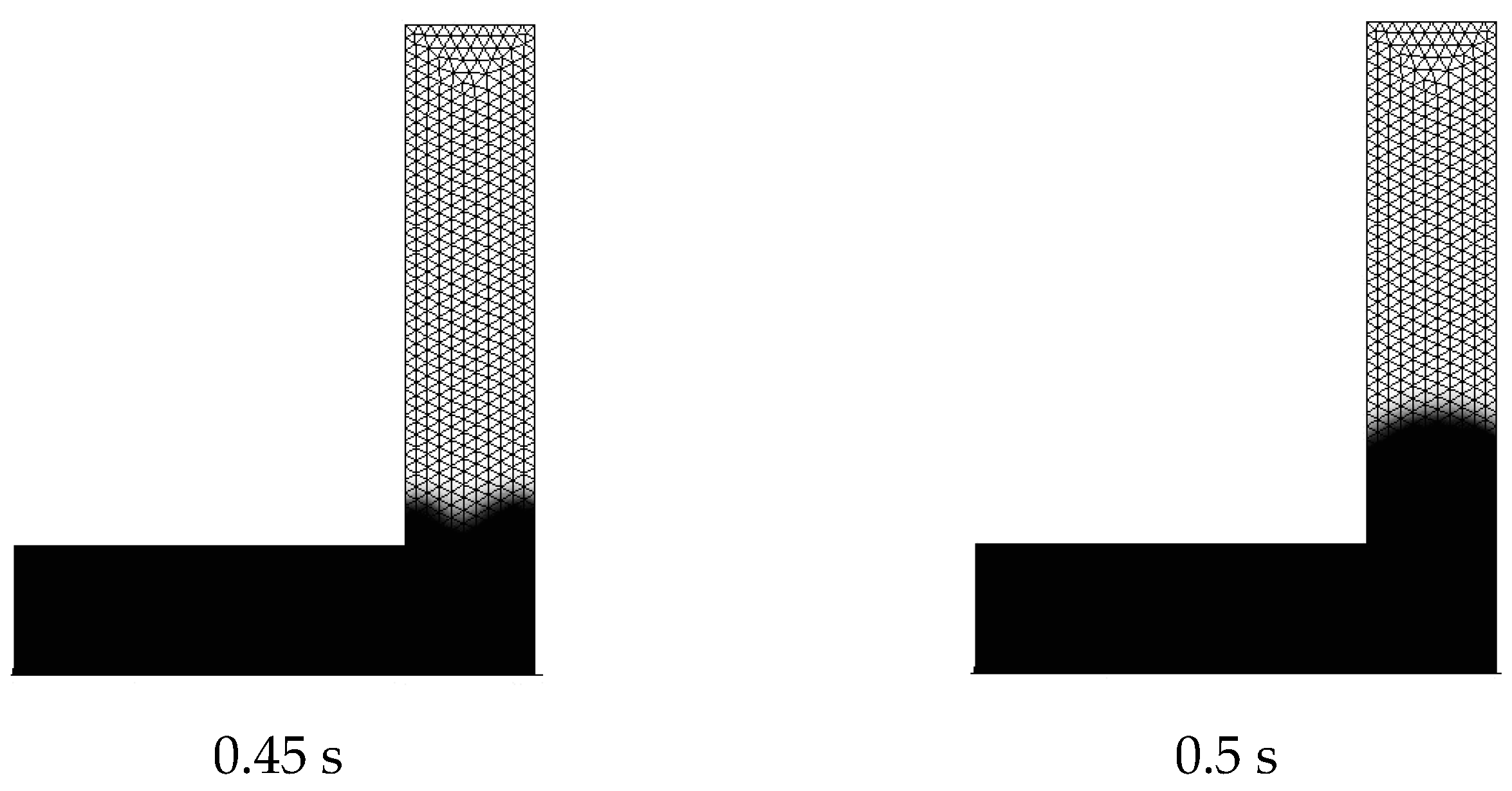However, in Figure 2, it is observed that the filling fronts arrive at bypass before merging together at the middle of bottom area in $\perp$ cavity. There exists an air gap between the two evolving fluid fronts that is not completely filled at the end of the simulation. For the case of channel in shape L, after the feedstock is horizontally injected into the mold cavity, it should arrive mainly at the right-hand side wall first, and then be extruded into the vertical part of the cavity. However, the same untrue phenomenon happens.

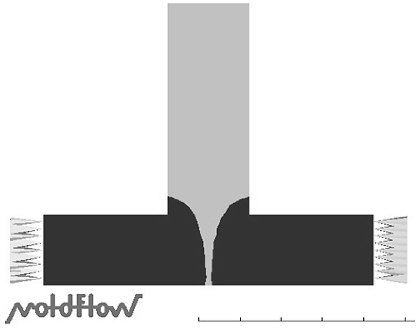
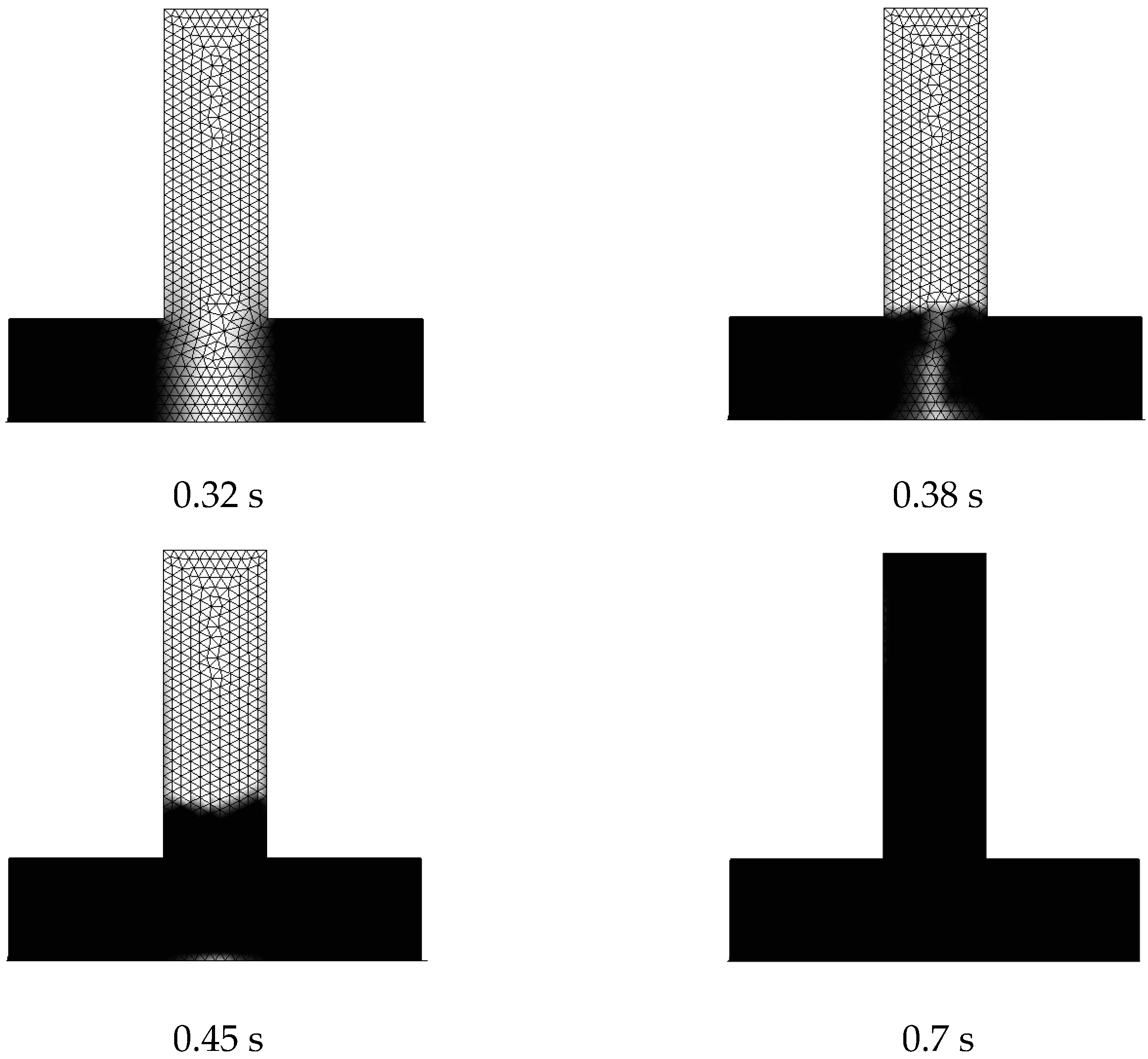
As another example, the simulation result made by commercial software MoldFlow® (Moldflow Corporation, Wayland, MA, USA) is introduced, as shown in Figure 3. It can be found that in the filling of a typical channel in shape $\perp$, the filling fronts from two opposite inlets arrived at the middle bypass before they joined together. Evidently this result does not match the real physical phenomenon. Although the software uses some strategy to modify this problem in post-processing steps, the filling patterns are not yet the true ones for the two opposite filling fronts to join together.

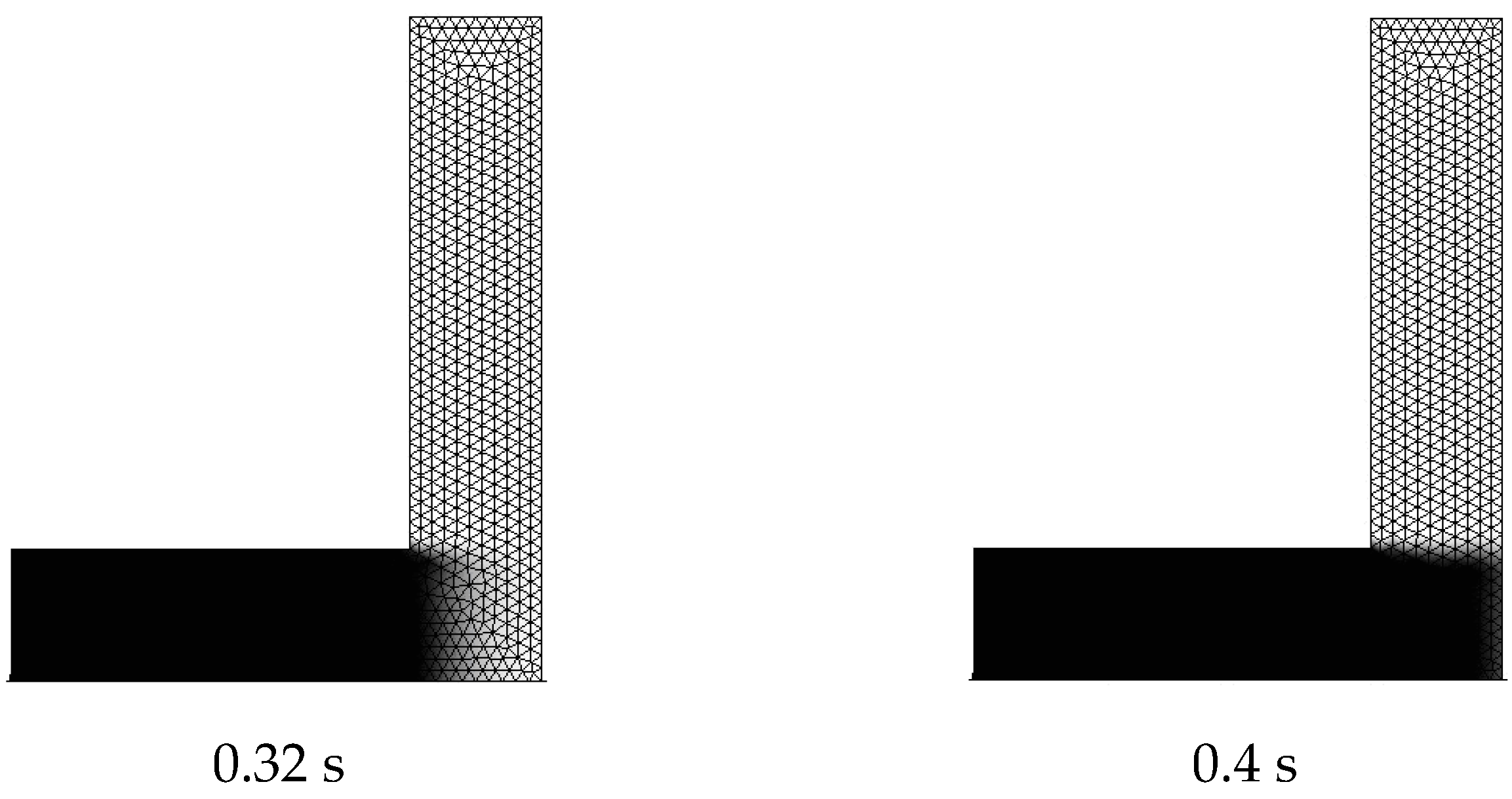
G. Larsen et al. [9] used the Streamline Upwind Petrov-Galerkin method (SUPG) to improve this filling problem, and confirmed that the simulation results are closer to the real situation than the ones by the Taylor-Galerkin method, which used previously by Barriere [10] and Cheng [11]. However, the real pattern of front joining in injection molding had not been exactly predicted, as shown in Figure 4.

The objective of the present study is to analyze the source for the untrue simulation results and find an effective way to settle the problem. A modified algorithm, which is similar to the upwind method [12,13], is proposed to trace the filling front. This proposed method makes the advection of the filling state to be mainly affected by the filling flow behind the filling front. Based on the finite element method and the efficient vectorial explicit algorithm developed by Cheng et al. [14], a systematic operation was proposed for modifying the velocity field ahead of the filling front, making the advance pattern of the flow front to be guided more on the flow of the feedstock instead of the fictive air flow. The simulation results in shapes like $\perp$ and L show that the proposed algorithm can effectively improve the untrue filling patterns in simulation.

2. Mechanical Models for PIM Process

2.1. General Definition

As usually chosen, an Eulerian description is adopted for the simulation of mold filling problems, which avoids the complicated and expensive remeshing procedures with Lagrangian descriptions. The general definition of mold filling problems is expressed as follows:

Let t ϵ [0,t₁] be an instant in the injection course, in which t₁ is the last moment of the filling process to reach the filled state. The sum of position X in the whole model is defined as set Ω. The set Ω in modeling of the injection molding consists of two different portions at each instant, the portion Ω_F filled by feedstock and the remaining space Ω_V taken by the air. A field variable F(x,t) is defined to represent filling state of the model at different instants. This field variable takes the value 1 to indicate the portion filled by feedstock and the value 0 for the remaining void portion, which contains air. The physical and geometrical definition for this modeling is shown in Figure 5, in which Γ₁ indicates the inlet of the mold, Γ_o represents the outlet through it, the air originally in the mold can be squeezed out during the injection. Γ_s represents for the intersection of subsets Ω_F and Ω_V which is, in fact, the filling front of the injection flow. V_I is the injected velocity on the inlet boundary. P_o is the pressure on the outlet boundary, which is set to be 0 in the present work to represent the environmental pressure.

2.2. Governing Equation for Filling Process and Evolution of Filling Front

To keep the uniqueness of the solution strategy and simplicity of the software structure, and under the frame of Eulerian description, the governing equations for the filling flow are chosen as the same for the filled and void portions of the injection model, except that the physical parameters are chosen differently for these two domains. The precondition to distinguish two different portions in the mold is to obtain the filling state field at each instant, which indicates whether or not the position is filled by the feedstock in the mold.

2.2.1. Subsection Advection Equation for the Filling State

The front position of filled domain is represented by the predefined filling state variable. Some authors call it as the variable of pseudo concentration or fictive concentration [15]. At each instant t in the injection course, the evolution of the filling state variable is dominated by an advection equation, driven by the velocity field:

$$\frac{\partial \mathit{F}}{\partial \mathit{t}}+\nabla \cdot \left({\mathit{V}}_{}\mathit{F}\right)=0$$

(1)

where V is the velocity vector, the boundary condition is F = 1 at the inlet of the mold. Its initial condition is F = 0 everywhere in the mold cavity, except for the inlet surface.

2.2.2. Momentum Conservation

The Navier–Stokes equation is used to represent the momentum conservation. For two portions filled with different materials in the mold, it is expressed as:

$$\forall X\in {\Omega }^F,{\mathsf{\rho }}_{\mathrm{P}}\left(\frac{\partial V}{\partial \mathit{t}}+V\cdot \nabla V\right)=-\nabla \mathit{P}+\nabla \cdot {\mathsf{\sigma }}_{\mathrm{P}}^{\prime }+{\mathsf{\rho }}_{\mathrm{P}}g$$

(2)

$$\forall X\in {\Omega }^V,{\mathsf{\rho }}_{\mathrm{a}}\left(\frac{\partial V}{\partial \mathit{t}}+V\cdot \nabla V\right)=-\nabla \mathit{P}+\nabla \cdot {\mathsf{\sigma }}_{\mathrm{a}}^{\prime }+{\mathsf{\rho }}_{\mathrm{a}}g$$

(3)

where ρ_p is the polymer density in the filled mold cavity, whereas ρ_a is the air density in the unfilled mold cavity, P represents the hydraulic pressure field, σ_p’ and σ_a’are the deviatoric Cauchy stress tensors in the filled and void portions, and g is the gravity vector.

As the flow in injection molding is often a problem with a small Reynolds number, sometimes the influence of the advection effect is negligible compared to the viscous effect in the Navier–Stokes equation. The momentum conservation can be then reduced to the solution of two distinct Stokes equations, expressed as:

$$\forall X\in {\Omega }^F,{\mathsf{\rho }}_{\mathrm{P}}\frac{\partial V}{\partial t}=-\nabla P+\nabla \cdot {\mathsf{\sigma }}_{\mathrm{P}}^{\prime }+{\mathsf{\rho }}_{\mathrm{P}}g$$

(4)

$$\forall X\in {\Omega }^V,{\mathsf{\rho }}_{\mathrm{a}}\frac{\partial V}{\partial t}=-\nabla P+\nabla \cdot {\mathsf{\sigma }}_{\mathrm{a}}^{\prime }+{\mathsf{\rho }}_{\mathrm{a}}g$$

(5)

It should be mentioned that the material properties for the air portion are chosen differently from their true values. Due to the singleness of the solution scheme for two different portions, it may result in the instability in the numerical solution if the mass and viscosity in the void portion are too different from the ones in filled portion. Thus, for the portion filled by the feedstock, material properties are the real ones. For the rest of the void portion, material properties should be modified to avoid too much of the difference compared to the ones in the filled portion. In fact, the result of the simulation in the void portion is not of our interest. Thus, the result of such a numerical treatment is acceptable.

The boundary condition should be imposed for each variable in the solution process. The mold inlet can be specified by a prescribed velocity or imposed pressure. On the mold outlet, one needs simply to impose a zero pressure, assigned to atmosphere pressure. For the boundary conditions on the mold walls, it is set to be a sticky wall. The velocity in both normal and tangent directions is set to zero.

3. The Source for Distorted Simulation Results

The filling processes may be distorted in the simulation by the following sources:

3.1. Differences in Physical Properties of the Feedstock and Air not Being Taken into Account in the Governing Equation of the Filling Evolution

An Eulerian description is used for simulation of the injection molding process. The filling state variable is governed by the advection equation to track the filling fronts. As in Equation (1), it does not distinguish the different effects of the feedstock and air on the advance of the filling front. Due to an extreme difference in the nature of these two substances, their effects on the evolution of the filling front are extremely different, too. In fact, as an incompressible fluid, the advance of the filling front is mainly driven by the flow of feedstock behind it, and rarely guided by the air flow ahead. However, the variable of filling state F is advected by the velocity field in the whole mold cavity in simulation. This means that the velocity ahead and behind the filling front represent the equal effect on the advance of the filling front. In fact, the pressure gradient is built up mainly in the flow of the feedstock, rather than in the air flow. The flow of air has much less effect on the advance of the feedstock filling front.

3.2. Artificial Air Properties Taken in Simulation

As Eulerian description is used for injection molding, a filling state variable governed by advection equation is defined to track the filling fronts. The void portion in the mold is supposed to be filled by a fictive fluid to simplify the procedures. Under the frame of an Eulerian description, and in order to keep integrity and consistency of the solution scheme, air in the void portion is also assumed to be as incompressible as the feedstock. By using this strategy, the computation of both the filled cavity and the void portion can be implemented with the unique numerical operation. However, the incompressible assumption for the air flow is not really consistent with its true nature. Such an assumption may also affect the advance of the filling front, other than its virtue to simplify the solution algorithm.

Additionally, the flow of materials in both filled and unfilled portions (air flow) should satisfy the conservation of momentum. In Equations (2) and (3) it can be noticed that, in these two parts, the same Navier–Stocks equation has been used, except that different material parameters are assigned. The large difference in the natures of feedstock and air may result in numerical instability. Thus, artificially increasing the mass and viscosity of air becomes a common practice to maintain the stability of the numerical simulation. Then, the inaccurate air flow may affect the advance of the filling front, leading the simulation results to be distorted. This is another factor to produce distortion in the simulation of the front tracking.

According to the analysis on the cause of distortion for front tracking, the problem is then how to make the advection of the filling state function depend more on the flow behind the filling front, and less on the flow of air ahead of the front.

4. Modification of the Solution Procedure

Based on the mechanical model and the notion of upwind method to strengthen the influences of the feedstock flow located behind the filling front, a notion similar to upwind method was introduced. A corresponding correction method was proposed to settle the distortion of filling front mentioned above. A feasible way to make the filling pattern more realistic is to modify the velocity field near the filling front. The advance of the filling front can be made to follow the guidance of the feedstock flow behind it, if the velocity just before the front is set to be similar to that behind the front. By means of a systematic operation to modify the velocity field for the filling simulation, the untrue impact of air flow, represented by the velocity field ahead of the filling fronts, can be reduced. To implement such method, there exist two key issues to be solved:

Firstly, how can we determine the band to be modified, ahead of the filling front?

The selection can be made by the unit of element, judging, and selecting element by element. In fact, according to the definition of field variable F(x,t), it takes the value F = 0 to indicate the void portion while F = 1 represents the filled one inside the mold cavity. Then the nodes located in the band close to filling front should represent the values between 0 and 1, note that F_Frt, 0 < F_Frt < 1. One can prescribe two values F_low and F_up to define the range of band before the front.

0 < F_low < F_Frt < F_up < 1

(6)

By example, for the 2D triangle elements with three nodes, an element can be regarded in the band if there exists at least one node for its F value to locate between F_low and F_up. Let Ω_Frt represent the band region (neighbor to the filling front). Assuming e being any one element in the model, i is the node number belong to this element:

$$\forall \mathrm{e},\forall i\mathsf{ϵ}\mathrm{element}\mathrm{e}{\mathit{F}}_{\mathrm{low}}<{\mathit{F}}_{\mathrm{Frt}}<{\mathit{F}}_{\mathrm{up}}\Rightarrow \mathrm{e}\mathsf{ϵ}{\mathsf{\Omega }}_{\mathrm{Frt}}\left(t\right)$$

(7)

as shown by the grey area in Figure 6.

Secondly, how do we modify the velocity field for computation of the filling state?

It is evident that the modified velocity fields are used only for the solution of the filling states. The modified velocity fields should be smooth and continuous ones. Otherwise, the solution of the advection equation will become unstable and produce spurious results.

A general smoothed procedure is proposed as follows:

$${\left\{\mathit{V}\right\}}_{\mathrm{F}}=\underset{\mathsf{\Omega }}{\mathrm{A}}{{\displaystyle \underset{{\mathsf{\Omega }}^{\mathrm{e}}}{\int }\left[\tilde{\mathit{N}}\right]}}^{\mathrm{T}}\left[\tilde{\mathit{N}}\right]\mathit{d}\mathsf{\Omega }{\left\{{\mathit{V}}^{\mathrm{e}}\right\}}_{\mathrm{F}}$$

(8)

where {V}_F is the velocity field, expressed in a discretized way at each node, for the solution of the filling state. Note that it is a modified and smoothed one to make the simulation of the front progress more realistic. {V^e}_F represents the column of velocity values at all nodes of an element. It initially takes the velocity values obtained by the solution of the Stokes equations, but these values are modified when the elements locate in the band ahead of the filling front. First, one node with a maximal F value will be determined as the upwind node, then the velocity value of the rest of the nodes in the same element will be replaced by the velocity value of the upwind node.

For an element in the band, element number e, and the node number i:

$$\begin{gathered} \forall \mathrm{e}\in {\mathsf{\Omega }}_{\text{Frt}}\left(\mathit{t}\right),\forall i\in \text{element e} \\ \exists k\in \text{element e},\mathrm{for}{\mathit{F}}_{\mathit{k}}={\left({\mathit{F}}_{\mathit{i}}\right)}_{\text{max}} \end{gathered}$$

(9)

where k is the upwind-stream node number, indicating that the node is of a maximum F value (Fi)max in the element.

$$\forall i\in \text{element e},\mathrm{let}{\mathit{v}}_{\mathit{i}}={\mathit{v}}_{\mathit{k}}$$

(10)

By this treatment to the velocity values of the elements located in the band, the velocity in thin layer elements ahead of the filling front is modified to be the values of elements behind. This operation reinforces the effect of the feedstock behind the flow front, while reducing the unrealistic guidance of the air flow. It represents more the real physical phenomenon, and it is more consistent with the true flow process.

For the details of different operators, let us take the triangle element of three nodes as a simpler example. These types of elements include three linear interpolation functions N₁, N₂, N₃.

The values of V at element level {V^e} take the following form:

{V^e}^T = {V₁₁ V₁₂ V₁₃ V₂₁ V₂₂ V₂₃}

(11)

The matrix of the interpolation function [Ñ] for velocity should be arranged in the corresponding form as:

$$\left[\tilde{\mathit{N}}\right]=\left\{\begin{array}{c}{\mathit{N}}_1\\ 0\end{array}\begin{array}{c}\\ \end{array}\begin{array}{c}0\\ {\mathit{N}}_1\end{array}\begin{array}{c}\\ \end{array}\begin{array}{c}{\mathit{N}}_2\\ 0\end{array}\begin{array}{c}\\ \end{array}\begin{array}{c}0\\ {\mathit{N}}_2\end{array}\begin{array}{c}\\ \end{array}\begin{array}{c}{\mathit{N}}_3\\ 0\end{array}\begin{array}{c}\\ \end{array}\begin{array}{c}0\\ {\mathit{N}}_3\end{array}\right\}$$

(12)

5. Validation of the Modification Scheme

5.1. Simulation Result of the Proposed Modification

This corrective strategy is carried out based on the explicit algorithm with fully vectorial operations [14], which was developed with the Taylar–Galerkin algorithm to solve the transport equation.

The feedstock density is set to be 711 kg·m⁻³, the viscosity is 20 Pa·s, and the velocity value imposed on the inlet is 0.1 m·s⁻¹ along the axial direction. The boundary condition is set to be a sticky wall, except on the inlet and outlet. These material properties and boundary conditions are assigned just for the purpose of software validation. They do not reflect the real values obtained from experiments.

By the proposed modification on the solution algorithm, the injection filling processes in channels of shapes $\perp$ and L are represented in Figure 7 and Figure 8. The filling duration for the $\perp$ shape and the L shape cavities are 0.7 and 0.8 s, respectively. A constant speed is imposed on the inlet. For the injection by incompressible flow, the filling volume should be proportional to the injection time until totally filled.

Figure 7 shows the injection process in channel of the $\perp$ shape. Feedstock is injected by two opposite inlets with the same speed. The filling fronts advance oppositely, join at middle of the cavity, first, and then go to the bypass together.

Figure 8 shows the result of the L-shaped channel by the modified method. The feedstock is horizontally injected into the mold cavity. It touches the wall at the right end first, and then is extruded into the vertical channel.

By comparison of the simulation results in Figure 3, Figure 7 and Figure 8, it is observed that the filling flows of the feedstock are more reasonable. They advance, join together, or touch the wall in front before being extruded into the bypass. The wrong guide of air flow to make the opposite feedstock flows going to bypass separately is largely reduced.

5.2. Comparison with Experiment Results

In order to show more about the validity of the above proposed method, experimental results from Larsen [9] are introduced to make a comparative analysis. The specific micro-injection molding machine, Battenfeld Microsystem 50, has been used in Arsen’s work to perform the molding process. A two-plate mold has been designed and manufactured. It has the dimensions indicated in Figure 9a. It is composed of three primary entities: the mold die cavity (Figure 9b) and ejectors (Figure 9c) for the mechanical ejection of small parts.

As the simulation took into account just the boundary wall condition in two dimensions, the depth of the T-type cavity is set to be a value much larger than the width; 8 mm for the depth was applied. Then, the wall effect in the third dimension on the filling front can be largely reduced to provide the comparison with simulation results.

Short-shots have been achieved for the injection process of a feedstock composed of binders PP, PW, and surfactant SA with a low density of 316L stainless steel metal powder. Feedstock injected volumes vary from 58 to 65 mm³. The comparison between results from the experiment and the improved simulation are shown in

Table 1. Comparison between results from experiment and the improved simulation.

Short-Shot of Experiment from 58 to 65 mm3	Simulation Result

.

From Table 1, it can be seen that the track of the filling flow is nearly the same as the experiment results. No clear differences appear in the whole filling process, including the instant when the two opposite flows merge together at the middle at the bottom in the $\perp$ cavity. Additionally, it can be completely filled at the end of simulation without any air gap between the two evolving flows. It can be regarded as an effective and true simulation result.

6. Conclusions

In order to improve the accuracy of the numerical simulation for the injection molding process, the source of the inexact filling fronts was analyzed. As the Eulerian description is generally used for filling flow problems, the governing equation of the filling state takes the form of the advection equation. The extreme difference in properties of the feedstock and air results in different effects for their flows on the advance of the filling front. This difference cannot be taken into account by the governing advection equation. The filling of feedstock may be wrongly guided by the flow of air, for some specific cases with the sudden change in flow direction of the feedstock. To settle the problem, a corrective method is proposed and implemented by the notion similar to the upwind method. Based on the efficient explicit algorithm for PIM simulations, a systematic operation is designed to modify the velocity field of the air flow close to the filling front for a solution of the filling advection equation. The untrue impact of air flow, represented by the velocity field ahead of the filling fronts, is significantly reduced. Then, the advance of the filling front can be mainly affected by the feedstock flow behind the filling front. The simulation results show that the corrective algorithm can effectively improve the distorted results. The simulation of filling processes in the complex cavities with channels in shapes like $\perp$ and L can be significantly improved.

References

- Abdullahi, A.A.; Choudhury, I.A.; Azuddin, M. Process Development and Product Quality of Micro-Metal Powder Injection Molding. Mater. Manuf. Process. 2015, 30, 1377–1390. [Google Scholar] [CrossRef]
- Sahli, M.; Millot, C.; Gelin, J.C.; Barriere, T. The manufacturing and replication of microfluidic mould inserts by the hot embossing process. J. Mater. Process. Technol. 2013, 213, 913–925. [Google Scholar] [CrossRef]
- Piotter, V.; Hanemann, T.; Heldele, R.; Mueller, M.; Mueller, T.; Plewa, K.; Ruh, A. Metal and ceramic parts fabricated by microminiature powder injection molding. Int. J. Powder Metall. 2010, 46, 21–28. [Google Scholar]
- Greiner, A.; Kauzlaric, D.; Korvink, J.G. Simulation of micro powder injection moulding: Powder segregation and yield stress effects during form filling. J. Eur. Ceram. Soc. 2011, 31, 2525–2534. [Google Scholar] [CrossRef]
- Liu, Q.S.; Jie, O.Y.; Liu, Z.J.; Li, W.M. Visualization and simulation of filling process of simultaneous co-injection molding based on level set method. J. Polym. Eng. 2015, 35, 813–827. [Google Scholar] [CrossRef]
- Hu, Z.X.; Zhang, Y.; Liang, J.J.; Shi, S.X.; Zhou, H.M. An efficient parallel algebraic multigrid method for 3D injection moulding simulation based on finite volume method. Int. J. Comput. Fluid Dyn. 2014, 28, 316–328. [Google Scholar] [CrossRef]
- Rokkam, R.G.; Fox, R.O.; Muhle, M.E. Computational fluid dynamics and electrostatic modeling of polymerization fluidized-bed reactors. Powder Technol. 2010, 203, 109–124. [Google Scholar] [CrossRef]
- Du, J.; Chong, X.Y.; Jiang, Y.H.; Feng, J. Numerical simulation of mold filling process for high chromium cast iron matrix composite reinforced by ZTA ceramic particles. Int. J. Heat Mass Transf. 2015, 89, 872–883. [Google Scholar] [CrossRef]
- Larsen, G.; Cheng, Z.Q.; Barriere, T.; Liu, B.S. A streamline-upwind model for filling front advection in powder injection moulding. In Proceedings of the 10th International Conference on Numerical Methods in Industrial Forming Processes Dedicated to Pro, Pohang, Korea, 13 June 2010; pp. 545–552.
- Barriere, T. Expérimentations, Modélisation et Simulation Numérique du Moulage par Injection de Poudres Métalliques. Ph.D. Thesis, Université de Franche-Comté, Besancon, France, December 2000. [Google Scholar]
- Cheng, Z.Q. Numerical Simulation on Metal Injection Moulding. Ph.D. Thesis, Southwest Jiaotong University, Chengdu, China, December 2005. [Google Scholar]
- Burman, E. A monotonicity preserving, nonlinear, finite element upwind method for the transport equation. Appl. Math. Lett. 2015, 49, 141–146. [Google Scholar] [CrossRef]
- Kao, N.S.C.; Sheu, T.W.H.; Tsai, S.F. On a Wavenumber Optimized Streamline Upwinding Method for Solving Steady Incompressible Navier-Stokes Equations. Numer. Heat Transf. Part B Fundam. 2015, 67, 75–99. [Google Scholar] [CrossRef]
- Cheng, Z.Q.; Barriere, T.; Liu, B.S.; Gelin, J.C. A new explicit simulation for injection molding and its validation. Polym. Eng. Sci. 2009, 49, 1243–1252. [Google Scholar] [CrossRef]
- Abdullah, S.; Li, Y.; Aftab, K. Upwind compact finite difference scheme for time-accurate solution of the incompressible Navier–Stokes equations. Appl. Math. Comput. 2010, 215, 3201–3213. [Google Scholar]
© 2016 by the authors; licensee MDPI, Basel, Switzerland. This article is an open access article distributed under the terms and conditions of the Creative Commons Attribution (CC-BY) license (http://creativecommons.org/licenses/by/4.0/).