Article

The Eh-pH Diagram and Its Advances

by
Hsin-Hsiung Huang
Metallurgical and Materials Engineering, Montana Tech, Butte, MT 59701, USA
Metals 2016, 6(1), 23; https://doi.org/10.3390/met6010023
Submission received: 29 July 2015 / Revised: 22 December 2015 / Accepted: 28 December 2015 / Published: 14 January 2016
(This article belongs to the Special Issue Hydrometallurgy)

Abstract

:
Since Pourbaix presented Eh versus pH diagrams in his “Atlas of Electrochemical Equilibria in Aqueous Solution”, diagrams have become extremely popular and are now used in almost every scientific area related to aqueous chemistry. Due to advances in personal computers, such diagrams can now show effects not only of Eh and pH, but also of variables, including ligand(s), temperature and pressure. Examples from various fields are illustrated in this paper. Examples include geochemical formation, corrosion and passivation, precipitation and adsorption for water treatment and leaching and metal recovery for hydrometallurgy. Two basic methods were developed to construct an Eh-pH diagram concerning the ligand component(s). The first method calculates and draws a line between two adjacent species based on their given activities. The second method performs equilibrium calculations over an array of points (500 × 800 or higher are preferred), each representing one Eh and one pH value for the whole system, then combines areas of each dominant species for the diagram. These two methods may produce different diagrams. The fundamental theories, illustrated results, comparison and required conditions behind these two methods are presented and discussed in this paper. The Gibbs phase rule equation for an Eh-pH diagram was derived and verified from actual plots. Besides indicating the stability area of water, an Eh-pH diagram normally shows only half of an overall reaction. However, merging two or more related diagrams together reveals more clearly the possibility of the reactions involved. For instance, leaching of Au with cyanide followed by cementing Au with Zn (Merrill-Crowe process) can be illustrated by combining Au-CN and Zn-CN diagrams together. A second example of the galvanic conversion of chalcopyrite can be explained by merging S, Fe–S and Cu–Fe–S diagrams. The calculation of an Eh-pH diagram can be extended easily into another dimension, such as the concentration of a given ligand, temperature or showing the solubility of stable solids. A personal computer is capable of drawing the diagram by utilizing a 3D program, such as ParaView, or VisIt, or MATLAB. Two 3D wireframe volume plots of a Uranium-carbonate system from Garrels and Christ were used to verify the Eh-pH calculation and the presentation from ParaView. Although a two-dimensional drawing is still much clearer to read, a 3D graph can allow one to visualize an entire system by executing rotation, clipping, slicing and making a movie.

1. Introduction

All Eh-pH diagrams are constructed under the assumption that the system is in equilibrium with water or rather with water’s three essential components, H(+1), O(−2) and e(−1); the oxidation states are presented using Arabic numbers with a + or a − sign. The diagrams are divided into areas, each of which represents a locally-predominant species. Eh represents the oxidation-reduction potential based on the standard hydrogen potential (SHE), while pH represents the activity of the hydrogen ion (H+, also known as a proton). An Eh-pH diagram can describe not only the effects of potential and pH, but also of complexes, temperature and pressures. By convention, Eh-pH diagrams always show the thermodynamically-stable area of water by two dashed diagonal lines.
Two typical Eh-pH diagrams, both based on thermodynamic data from the NBS database [1], are presented. Figure 1 shows an Eh-pH diagram for one component (excluding three essential H(+1), O(−2) and e(−1) components) of metal, in this case manganese, Mn, while Figure 2 is that of another component of mineral acid phosphorus, P. Both diagrams show that oxidized species reside in high Eh areas, while reduced species are in low Eh areas. The metal diagram starts, at the left edge, from metal ions (Mn2+) at low pH, which progressively react with OH- as pH increases to produce metal hydroxides (Mn(OH)2) or oxides. The diagram for the mineral acid starts, again from the left, with acid (H3PO4) and progressively deprotonates due to reactions with OH- to finally produce phosphate ion (PO43-) at high pH. Figure 1 also illustrates the tendencies to transition between species.
Figure 1. Eh-pH diagram of a Mn–water system. Dissolved manganese concentration, [Mn] = 0.001 M.
Metals 06 00023 g001
Figure 2. Eh pH diagram of a P-water system. Dissolved phosphorus species, [P] = 0.001 M.
Metals 06 00023 g002

Scope of the Paper

This paper illustrates some ways to improve a basic Eh-pH diagram for better visualization of species and stability regions. The demonstrated methods are all calculated and constructed with an ordinary PC, without a high-end graphics card, using Windows 7 or a higher version. All diagrams can be obtained in a short time. The fundamentals underlying the calculations are briefly described and/or available in the literature and listed as references. Discussions include:
  • Examples of applications: geochemical formation, corrosion and passivation, leaching and metal recovery, water treatment precipitation and adsorption.
  • Development of equilibrium line and mass balance point methods to handle ligand component(s): the theory, illustration and result comparison are presented; both methods satisfy the Gibbs phase rule derived for the Eh-pH diagram.
  • Examples by merging two or more diagrams for better illustration of the overall reactions involved in a process.
  • Demonstrations using a third party program to produce 3D diagrams with the addition of a third axis. The axis can represent the solubility of stable solids, ligand concentration or temperature. Two 3D wireframe volume plots of the Uranium-carbonate system based on a classic Garrels and Christ [2] work were used to verify the Eh-pH calculation and the presentation from ParaView.
This paper is not intended to discuss the following topics in detail:
  • Comparison among existent computer programs listed from the literature that directly or indirectly construct an Eh-pH diagram.
  • Effects from temperature, pressure, ionic strength and surface complexation for aqueous chemistry.
  • The algorithm and flow sheet to construct the diagram used by the author: they are available and referenced elsewhere; no source codes of the programs are presented.
  • Comparison or comments on third party 3D programs used by the author.
Note: The diagrams shown in this paper are solely for illustration. Unless specified, all were constructed at a temperature of 25 °C and zero ionic strength. The molarity is used for a dissolved species as [species], and Σcomponent is used to represent the sum of all mass from one component. Various thermodynamic databases were used as was convenient. Except as noted for 3D plots, all diagrams were constructed by STABCAL [3] running on the Windows operating system using win8.1 64 bit, Pentium i7, 4.3 GHz with 16 GB RAM hardware, and 1680 × 1050 resolution monitor.

2. Crucial Developments of the Eh-pH Diagram

Chapter 2 of the Pourbaix Atlas [4] presented the method of calculation and the procedure of the construction of an Eh-pH diagram. The process was relatively simple since only one component was considered.
Garrels and Christ [2] dedicated a full chapter to the Eh-pH diagrams. Several diagrams related to geochemical systems were not only presented, but also explained. They laid out a procedure to construct the diagrams when ligand(s) were involved, such as illustrated in the Fe–S and Cu–Fe–S systems. They also presented two 3D wireframe volume diagrams for the Eh-pH-CO2 system, which will be discussed later in this paper.
A crucial development in constructing an Eh-pH diagram was in deciding how to handle a system when a ligand component was involved. Two completely different approaches were evolved.

2.1. Development of the Equilibrium Line Method

The equilibrium line method was originally used by Pourbaix for simple metal-hydroxide systems. Each line equation is derived from an electrochemical and/or acid-base reaction between species.
Garrels and Christ used Fe–S as an example to show that the same procedure presented by Pourbaix could be applied to a multicomponent system. Basically, it involved two separate steps: domain areas of ligand S were first constructed, then all Fe species (including Fe–S complexes) were distributed in each isolated area of the ligand species. Huang and Cuentas [5] presented a computer algorithm to construct this type of diagram using an early personal computer.

2.2. Development of the Mass Balance Point Method

Forssberg et al. [6] constructed several Eh-pH diagrams related to chalcopyrite, CuFeS2, by performing equilibrium calculations for the whole system at once at each given Eh and pH. By doing so, the Cu:Fe:S ratio could be strictly maintained to 1:1:2 at all points. They used the SOLGASWATER program developed by Eriksson [7] to perform the calculation. This point-by-point mass balance method identifies the predominant species at each given point of Eh and pH. Points of the same species were combined into an area for the final diagram. The SOLGASWATER program used free energy minimization, which is commonly used for equilibrium calculation. Woods et al. [8] also presented diagrams for the Cu–S system using SOLGASWATER.
The mass balance method can also be computed considering the law of mass action (Huang et al. [9]). This approach simultaneously solves all equations, equilibria and mass balances, at each given point of Eh and pH. As with the free energy minimization method, the final diagram has to be plotted by grouping calculated results together. presented later, was reconstructed using the law of mass action for Cu–S and matched with from Woods et al. [8].
Besides matching the mass input, these diagrams reveal the presence of multiple solids as restricted only by the Gibbs phase rule. The key to the success of using the point-by-point method, however, is the resolution of the grids used in the calculation. Except for 3D diagrams, all mass balance diagrams in this paper were constructed using grids of at least 400 × 800.

3. Applications for the Diagrams

Eh-pH diagrams are widely used in many areas where an aqueous system is affected by oxidation-reduction and/or acid-base reactions, ligand complexation, temperature or pressure. The following three examples are presented to illustrate these effects.

3.1. Geochemical Formation

Copper porphyry ore deposits occur throughout the world and are very important sources of copper, silver and gold. These deposits initially consist of disseminated sulfide minerals in a rock matrix, but near-surface weathering oxidizes the sulfides and leaches dissolved metals from the residual mass. These leached metals in solution percolate downward and are often reprecipitated in an enrichment zone overlying unreacted sulfide protore. The near-surface weathered, oxidized portion of the deposit corresponds to the oxidizing region of an Eh-pH diagram, while the non-oxidizing reduced enrichment zone corresponds to the reducing diagram region. Figure 3 is a geologic sketch of an idealized porphyry deposit versus the depth from the surface, while Figure 4 is a copper Eh-pH diagram in which iron, sulfur and carbonate, besides copper, are considered in the calculations. The minerals predicted in the diagram, solely from thermodynamic considerations, correspond extremely well with minerals observed in these deposits and with the relationships between these minerals. In the oxidized and weathered zone, the original copper and iron sulfides are not stable, while copper carbonates (antlerite, malachite, azurite) and oxides (tenorite, cuprite) form instead. In the enrichment zone, the copper-only sulfides covellite (CuS) and chalcocite (Cu2S) are dominant, with native copper seen to occur in both oxidized and enriched zones.
Figure 3. Illustrated copper ore deposit for comparison to the Eh-pH diagram to the right (Dudas et al. [10]).
Metals 06 00023 g003
Figure 4. Eh-pH diagram Cu–CO2–Fe–S in water. pCO2 = 0.1 atm, [S] = 0.01 M, [Fe] = [Cu] = 0.001 M. Species were taken from the LLnL database [11].
Metals 06 00023 g004
Another geochemical example is the Eh-pH diagram modeling metamorphic conditions. In order to show the effect of high pressure, a database such as SUPCRT (Johnson et al. [12]) is required. See the reference from Kontny et al. [13] for a Fe–S diagram at 300 °C and 1500 bars pressure or Huang [14] for more calculations and examples using SUPCRT-related databases.

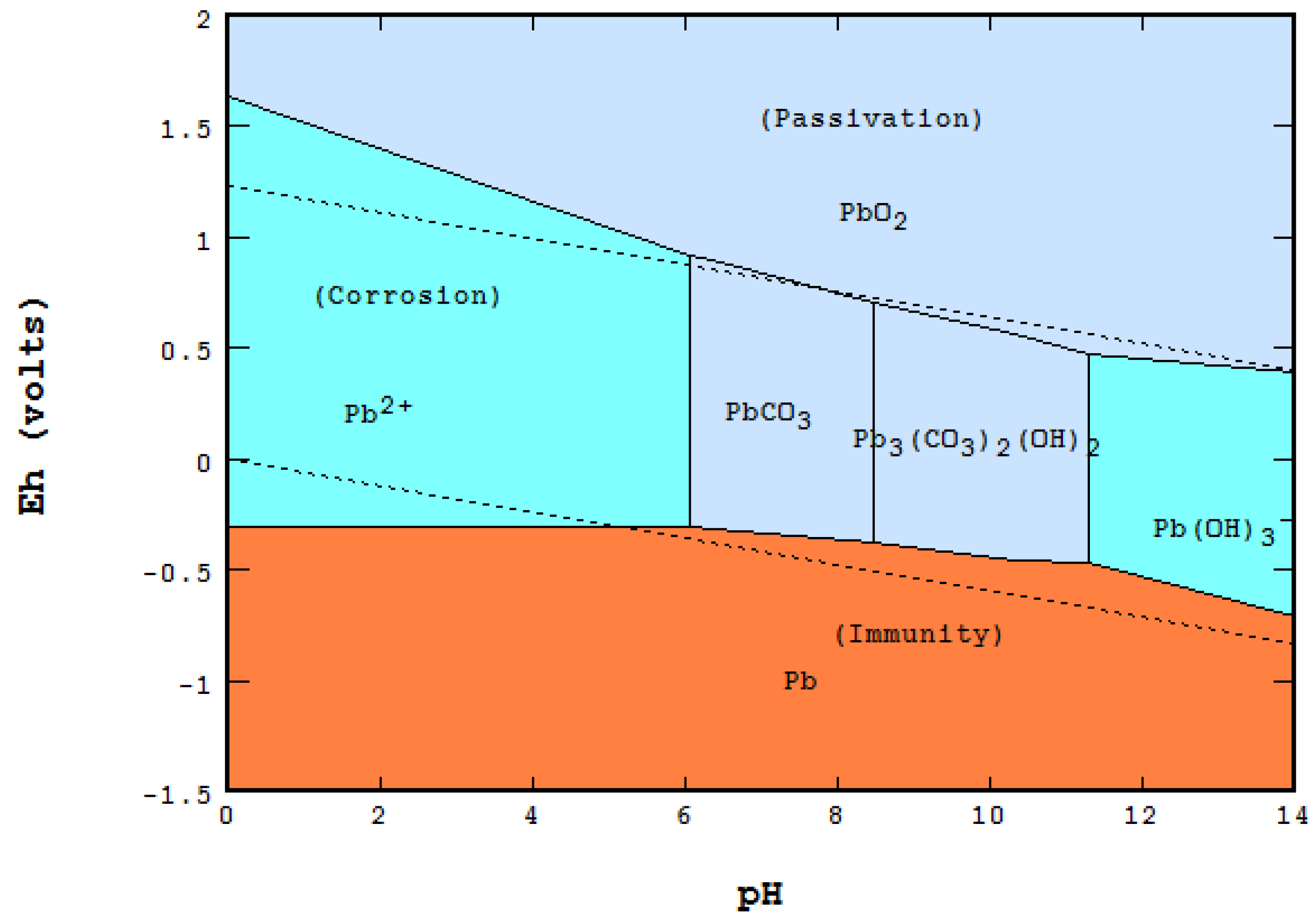
3.2. Corrosion and Passivation

Metallic corrosions are widespread problems of great importance in virtually all physical structures. Corrosion chiefly occurs when metal electrochemical dissolution is favored. One way to protect the metal from corrosion is to form a passivated layer, which may simply be a metal oxide. Some metal oxides, such as PbO, exhibit relatively high solubility and provide little corrosion protection.
The distribution-pH diagram (Figure 5) shows the concentrations of dissolved Pb species, as well as the solubility of PbO, versus pH. Formation of metal-carbonate, as shown in the Eh-pH diagram of Figure 6, offers a wider passivation region. Both diagrams were constructed using the LLnL [11] database. Pourbaix in his lectures [15] presented a similar case for using CO2 to passivate Zn metal.
Figure 5. Solubility of PbO (shaded) versus pH. PbO does not provide good corrosion protection, even at elevated pHs.
Metals 06 00023 g005
Figure 6. Eh-pH of the PbCO3–water system. [Pb] = 1 × 10⁻⁶ and [CO3] = 0.001 M. Pb carbonate phases do provide corrosion resistance.
Metals 06 00023 g006

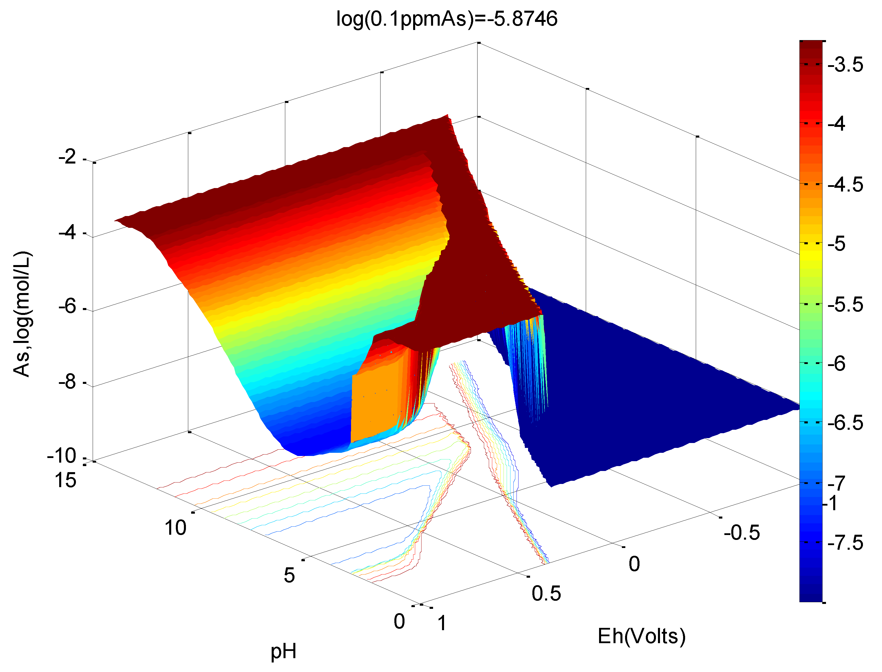
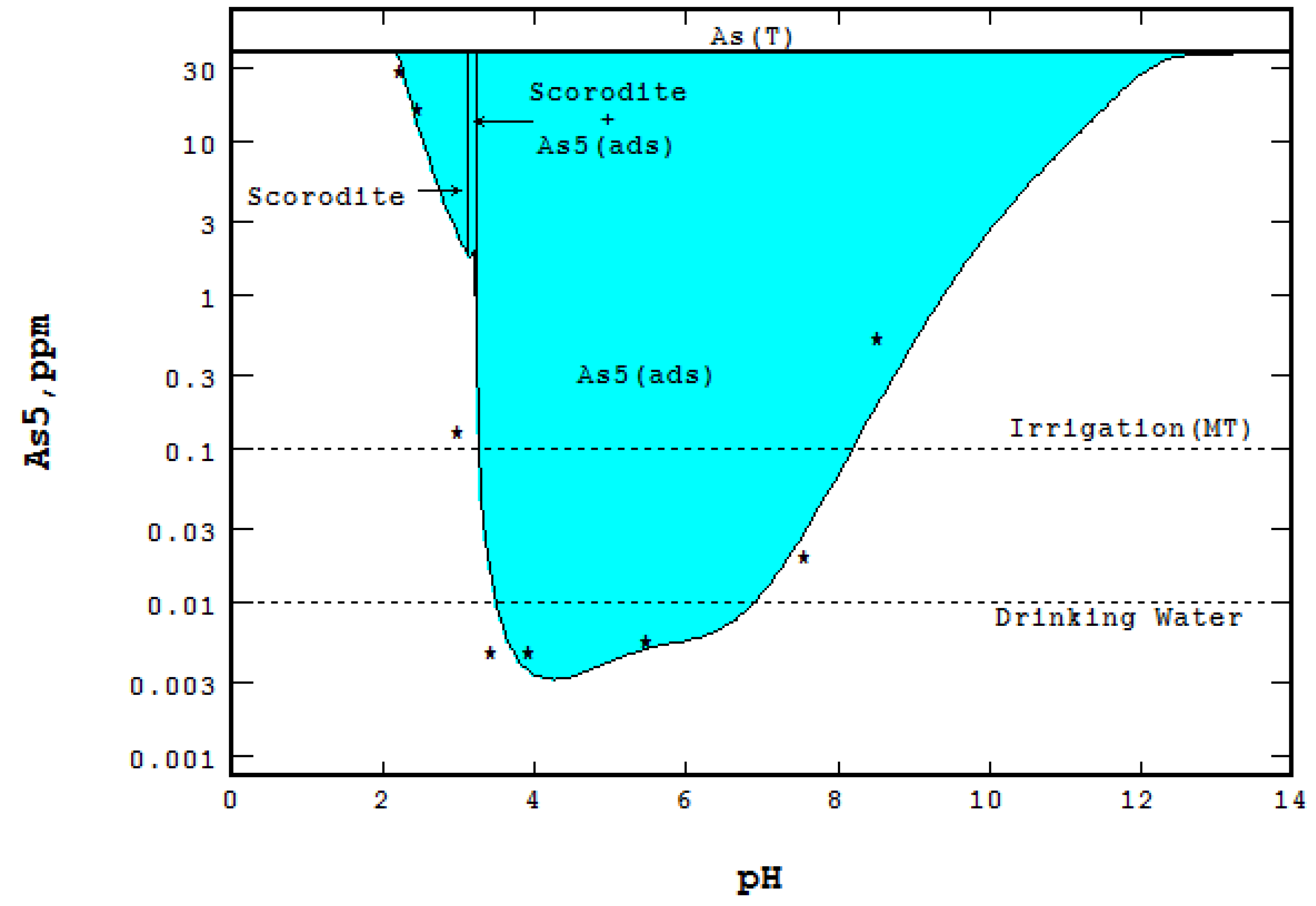
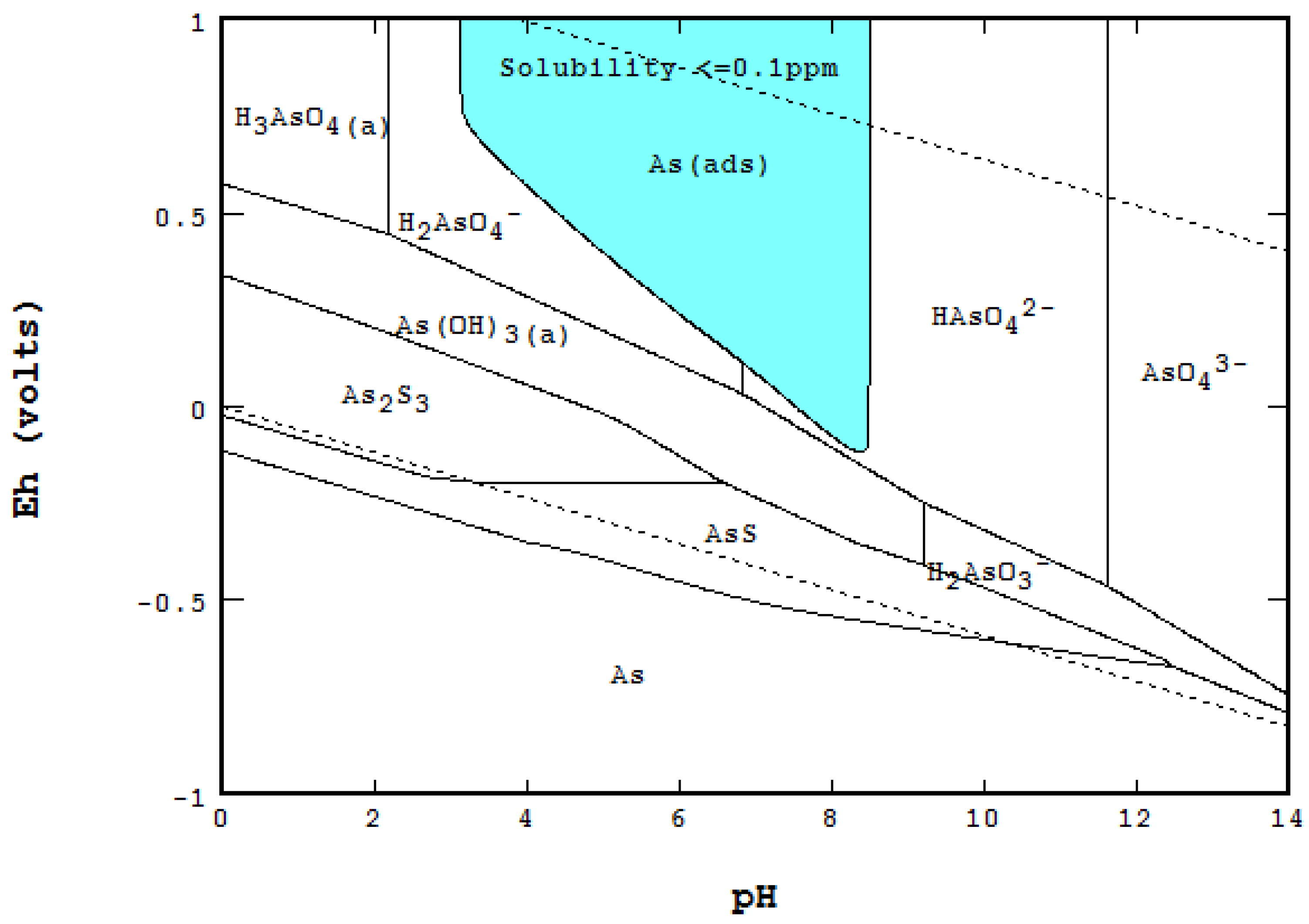
3.3. Water Treatment and Adsorption

Water discharge standards almost always include concentration limits for the acid, base and heavy metals. When feasible, precipitation of a solid, followed by a liquid-solid separation is usually the preferred means of achieving these limits, but often, stringent standards are difficult, if not impossible, to comply with by this means. Adsorption onto metal oxides/hydroxides sometimes provides an alternative means of removing these metals from the discharge solution. The adsorption of arsenic (As) by ferrihydrite is demonstrated in Figure 7 using data from Nishimura et al. [16]. For this particular experiment, the initial conditions were ΣAs = 37.5 mg/L with a Fe/As mole ratio of 10. The source of ferric iron was dissolved Fe2(SO4)3:5H2O.
The species considered and their thermodynamic values were also taken from the LLnL database [11]. The equilibrium calculation included adsorption using a surface complexation model. Potentially adsorbed species onto ferrihydrite are three arsenates, one arsenite, two sulfates, hydrogen ion and hydroxide. Their equilibrium constants, logKadsint, were obtained from Dzombak and Morel [17]. In order to better fit the experimental data, some modifying changes were made:
  • Type 2 site density for ferrihydrite was changed from 0.2 to 0.3 mole As/mole Fe due to co-precipitation,
  • The logK1int for adsorbed species ≡FeH2AsO4 was changed from 29.31 to 31.67,
  • The adsorbed species ≡FeAsO42− and its logK3int = 21.404 were added and
  • Solid scorodite (FeAsO4:2H2O) and its ΔG025C = −297.5 kcal/mole were included with the LLnL dbase.
Figure 7 is the resulting distribution-pH diagram, of the same type as Figure 5, for arsenate As(V). The adsorption model nicely matches the experimental data, demonstrating effectively what the arsenic removal should be. The adsorption of arsenite As(III), while not shown, also matches the experimental data. Figure 8 is presented to illustrate the Eh-pH diagram for the As–Fe–S–water system constructed using the mass-balanced (600 × 800 grids) method. The areas in light blue show solids and adsorbed species to a dissolved concentration less than 0.1 ppm.
Figure 7. Distribution of As(V) vs. pH diagram when Fe/As = 10. Asterisks are experimentally-observed values. Drinking water standard from EPA (2001).
Metals 06 00023 g007
Figure 8. Eh-pH of As–Fe–S water where the mole ratio of Fe/As = 10. The colored area indicates less than 0.1 ppm concentration of As by adsorption.
Metals 06 00023 g008

3.4. Hydrometallurgical Leaching and Metal Recovery

Three applications for hydrometallurgy are presented in more detail later in the section titled “Enhancing the Eh-pH Diagrams by Merging Two or More Diagrams”. These are:
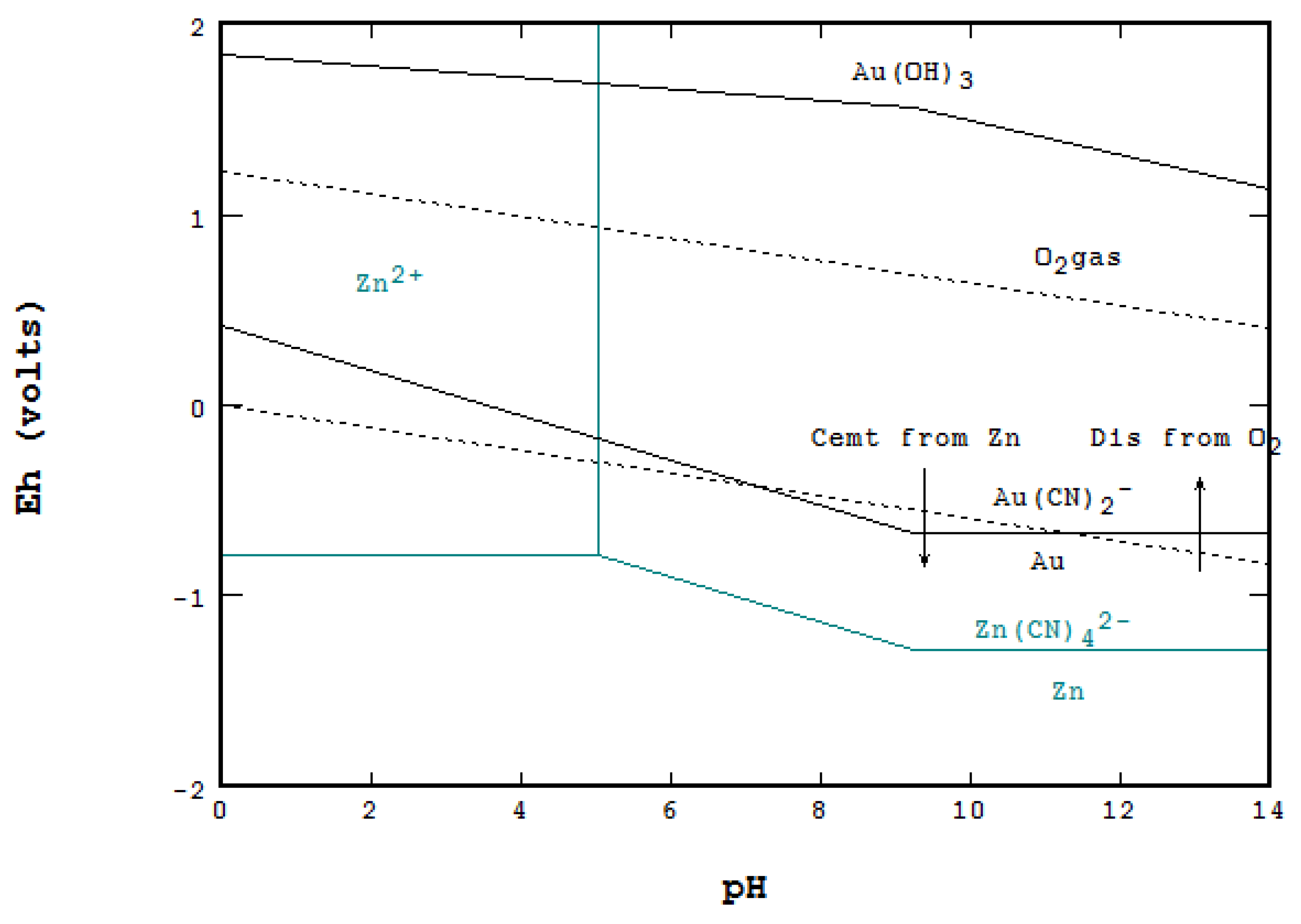
  • Cyanidation of Au and cementation with Zn Metal,
  • Cementation of copper with elemental Fe, and
  • Galvanic conversion of chalcopyrite with Cu metal with two construction methods for Eh-pH diagrams to handle ligand components.

4. Descriptions and Comparison between These Two Crucial Methods

4.1. Equilibrium Equations for Eh-pH Diagrams

The chemical equation between Species A and B in the water system, with or without electron involvement, can be expressed as:
aA + cC ↔ bB + dD + hH+ + wH2O (+ne)
Species C and D are ligand and complexes produced with ligand. The stoichiometric coefficient of a species is taken as positive if it is on the right-hand side of the equation, and vice versa. Species H+, H2O and e- may not always be on the right-had side of the equation. Because so many equations and species are involved while performing equilibrium calculations for an Eh-pH diagram, it is easier to use the free energy of formation of each involved species, ΔGi0, then to calculate the free energy of reaction as,
ΔGrex = ∑(υi × ΔGi0)
where υi represents the stoichiometric coefficient of species i.
Depending on whether or not the reaction involves an electron and/or hydrogen ion, the equations are:
The Nernst equation for oxidation-reduction reaction with or without acid-base:
Eh = Eh 0 + ln ( 10 ) R T ( n × F ) × [ log ( { B } b { D } d { A } a { C } c ) hpH ]
where Eh 0 = Δ G rex ( n × F ) , where R is the universal gas constant, 8.314472(15) J/(K·mol); T is in kelvins; F is the Faraday constant 96,485.3399(24) J/(V·equivalent); and {A} and the others species are defined as the activities of Species A. The activities of solid and liquid are normally assumed to be one; gas is taken as the atmosphere (atm). The activity of an aqueous solution is the multiplication of the concentration in mol/L, symbolized as [A], with its activity coefficient. The coefficient can be computed from one of the appropriate models. Without having the acid-base, the “hpH” term in the equation will be dropped out.
The equilibrium equation for acid-base reaction without redox reaction:
pH = 1 h × [ log ( { B } b { D } d { A } a { C } c ) + Δ G rex ln ( 10 ) × R T ]
The equation for reaction involves neither an electron nor a hydrogen ion:
log   Q log   K = log ( { B } b { D } d { A } a { C } c ) + Δ G rex ln ( 10 ) × R T
Species A will be favored if logQ − logK is positive, and vice versa.
As mentioned earlier, two different approaches may be used to construct an Eh-pH diagram. One is to calculate equilibrium equations between pairs of species and to construct the diagram by plotting the resulting equilibrium lines. The other is to perform equilibrium calculations from all involved species at each point in a grid, then selecting the predominant species at each point. Regardless of which method is used, these equilibrium equations have to be satisfied.

4.2. Line Method Using Equilibrium Concentration [5]

The diagram is constructed by computing the equilibrium between two adjacent species from their activities. The concentration or activity of aqueous species has to be given. Figure 9 shows the Eh-pH diagram for Cu at three different concentrations. The case where a ligand component is also involved is demonstrated in Figure 10, for the Cu–S–water system using [S] = 0.001 and [Cu] = 0.001 mol/L. The areas of predominance for the various ligand S species (labeled in light blue) were first constructed. The distribution of Cu species, including Cu–S complexes, in each S domain (such as the area of H2S shaded with light blue) was then constructed. The final diagram of Cu species was determined by combining all of the areas from S ligands. It should be noted that the total concentration of ΣS may change depending on whether or not Cu is complexed with S. When Cu species are not complexed with S, ΣS would be 0.001 mol/L, as described. However, when Cu species are complexed with S, as in the formation of CuS, ΣS will be the molar sum of the S concentration plus the CuS concentration, which will be equal to 0.002 mol/L. In such a case, the mass of total S may not be constant, as originally assigned.
Figure 9. Eh-pH of Cu-water constructed by the line method where three concentrations in log scale are plotted. Data taken from NBS [1].
Metals 06 00023 g009
Figure 10. Eh-pH of Cu(main)–S (ligand). The line method plots the ligand first, shown in blue color. The distribution of Cu species for each domain of S is then determined.
Metals 06 00023 g010

4.3. Point-by-Point Method Using Mass Balance [9,18]

In this method, mass balances are considered and calculated with all of the equilibria from all of the components at once from every point of the grid. Unlike the line method where the concentration or activity of aqueous species is specified, this method requires knowing the total mass of each component. The calculation requires not only satisfying all equilibrium equations, but also matching all of the mass balances. The results are sorted out in order to plot the diagram for each specific component. This type of diagram is particularly important for Eh-pH diagrams, which include solids with composition ratios that are close to mineral formation ratios (such as 3:1:4 mole ratios for enargite Cu3AsS4)
Mass inputs, including masses of ligands, are crucial for determining critical areas of these diagrams. Figure 11 and Figure 12 illustrate this for the Cu–S–water system (data from NBS [1]). Figure 11 shows the case where S is stoichiometrically slightly less than copper, i.e., ΣCu = 0.001 and ΣS = 0.0009 M, while Figure 12 shows the case where S is slightly in excess. The higher mass of S leads to a larger area of predominance for CuS.
Figure 11. Mass-balanced Eh-pH diagram for the Cu–S–water system with copper slightly in excess. ΣCu = 0.001 M and ΣS = 0.0009 M.
Metals 06 00023 g011
Figure 12. Mass-balanced Eh-pH diagram for the Cu–S–water system with copper slightly in deficit. ΣCu = 0.001 M and ΣS = 0.0011 M.
Metals 06 00023 g012

4.4. Differences and Comparison between the Methods

Different results of the two methods can be seen by comparing diagrams constructed within the Cu–S system, with sulfate species not shown due to unfavorable kinetics (Woods et al. [8]). Figure 13 was constructed by the equilibrium line method where [Cu] = 0.118 and [S] = 0.059, and Figure 14 was constructed by the mass-balanced point method where ΣCu = 0.118 and ΣS = 0.059. Free energy data were taken from Woods et al. [8]. Crucial differences can be seen in the general area of Cu–S solids. As can be seen from Figure 13, even though the concentration ratio of Cu/S is specified as two to one, CuS, not Cu2S, is the predominant species.
The mass-balanced point calculation involved points on a 400 × 800 grid to a precision of 1 × 10⁻¹⁰, but took less than three minutes for a PC from creating a worksheet for input to plotting the final diagram.
Figure 13. Eh-pH diagram for the Cu–S–water system constructed by the equilibrium line method.
Metals 06 00023 g013
Figure 14. Eh-pH diagram for the Cu–S–water system constructed by the mass-balance point-by-point method. This diagram matches Figure 5 of Wood et al. [8].
Metals 06 00023 g014
The equilibrium line method was favored in the past due to its relative ease of construction. When diagrams were constructed using manual calculation (as by Pourbaix), the equilibrium line method was the only practical approach. As greater computational power became available, the mass-balanced point-by-point method came into favor. The following list includes some areas where the mass balance method should be considered over the line method.
  • When the exact composition of the system is needed: Examples include leaching and flotation studies. See Huang and Young [18] for more examples. The Eh-pH diagram of enargite (Cu3FeS4) (Figure 15) was constructed using data collected by Gow [19].
  • When a system is required to specify total concentration, not equilibrium concentration nor activity.
  • When the adsorption by solids, such as ferrihydrite, is considered (refer to Figure 8).
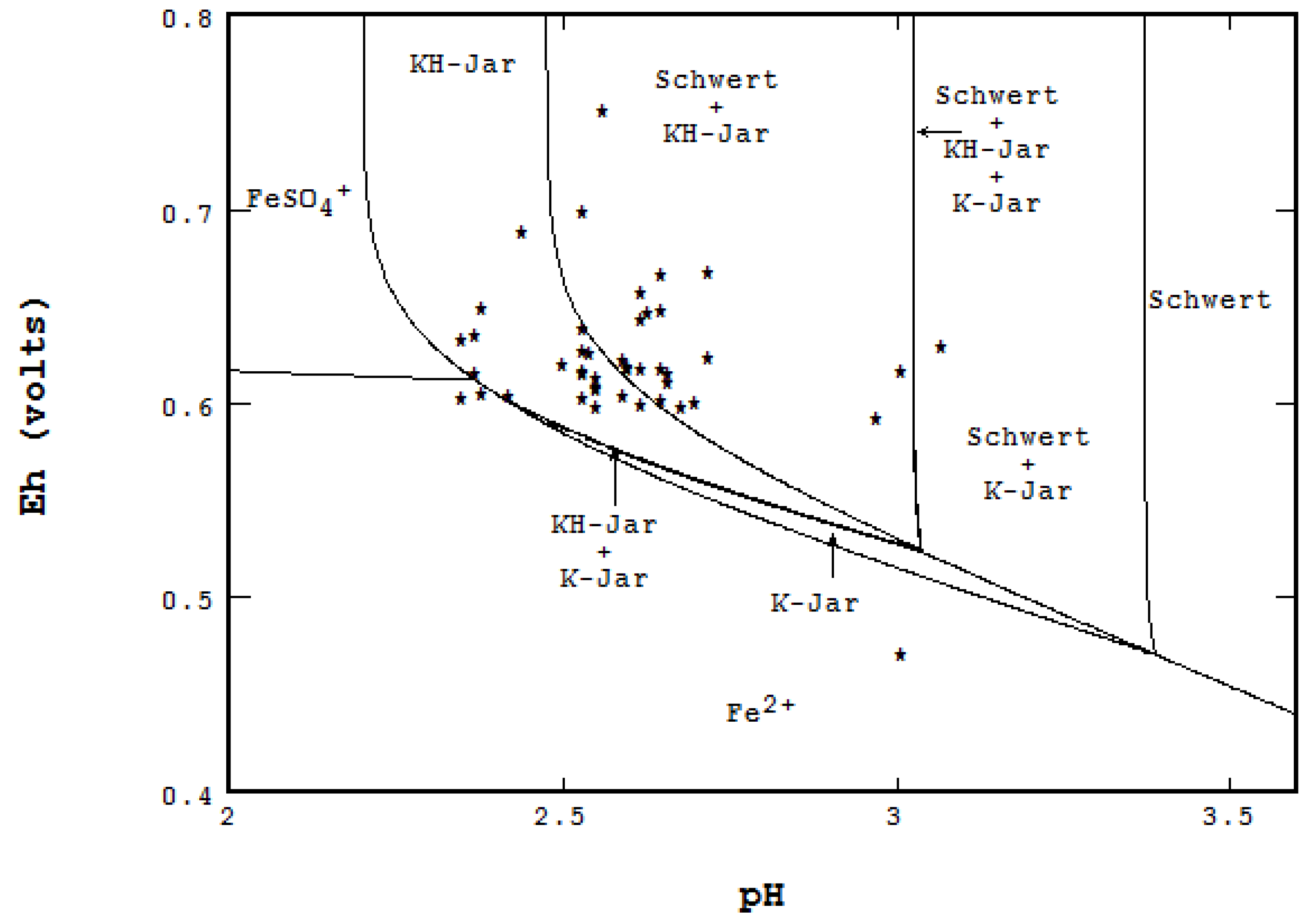
  • When multiple phases of a solid need to be shown: Figure 16 was constructed by showing the coexistence of schwertmannite with various forms of jarosites in Berkeley pit water. Water samples were taken and analyzed from 1987 to 2012 by the Montana Bureau of Mines and Geology [20], and the thermodynamic data for the solids species were regression estimated by Srivastave [21].
  • A diagram will most likely be mass balanced if a speciation program, such as PHREEQC (USGS) [22], was used to construct it. Results from the program were collected manually or electronically, then combined into an Eh-pH diagram.
Figure 15. Mass balanced Eh-pH diagram for the enargite Cu3AsS4 system. The mass ratio is 0.75:0.25:1 for Cu, As and S. The diagram shows only the copper species in acid solution.
Metals 06 00023 g015
Figure 16. Mass balanced Eh-pH diagram for the Fe–K–S system at 7 °C. This diagram shows the coexistence among schwertmannite, K-jarosite and KH-jarosite. * represents the data analyzed from the sampled water.
Metals 06 00023 g016
Both methods, however, can produce identical diagrams under the following conditions:
  • A one-component system, such as Figure 1 for Mn and Figure 2 for P,
  • The concentration of ligand component(s) is much greater than the main component, such as metal corrosion by sea water, and
  • Gas is the only ligand, such as the Fe–CO2(g) system.

4.5. Gibbs Phase Rule Applied to an Eh-pH Diagram

An Eh-pH diagram constructed using either method must follow the Gibbs phase rule. The original phase rule equation, P + F = C + 2, was developed for considerations of temperature and pressure. It can be refined for use in constructing an Eh-pH diagram by implementing some concepts and restrictions.
Mass-balanced method: This method calculates equilibrium from all components at once. The variables are as follows:
  • P is the total number of phases = 1 (liquid water) + 1 (gas if considered) + N (maximum number of solids/liquids),
  • F is the degree of freedom on the diagram, which is two for an open area, one on a boundary line and zero on a triple point,
  • C is the total number of components = 3 + EC (extra components). Three components are essential for Eh-pH calculation in an aqueous system. These are H(+1), O(−2) and e(−1). The extra components include the main component to be plotted, as well as all ligands.
  • The term of +2 is for temperature and pressure variables. Since both are considered to be constant, +2 will be dropped off. If any system involved a gaseous species, +1 should be used, but it will be canceled out with one extra gaseous phase to the equation.
The phase rule equation for an Eh-pH diagram, best expressed as the maximum number of solids plus liquids excluding the liquid phase of water, thus becomes:
Nmaxsolid = CF − 1
Example 1, Cu and S two-component system: The incorporation of the rule is illustrated in Figure 17, in which all solids containing Cu, as well as S components are presented. Since the method computes equilibria from all components involved at once, C = 3 + 2 and Nmaxsolid = 5 – F – 1 or 4 – F.
1a.
In an open area of the diagram where F = 2, Nmaxsolid will be equal to two. The co-existence of two solids can be seen in many places on the diagram,
1b.
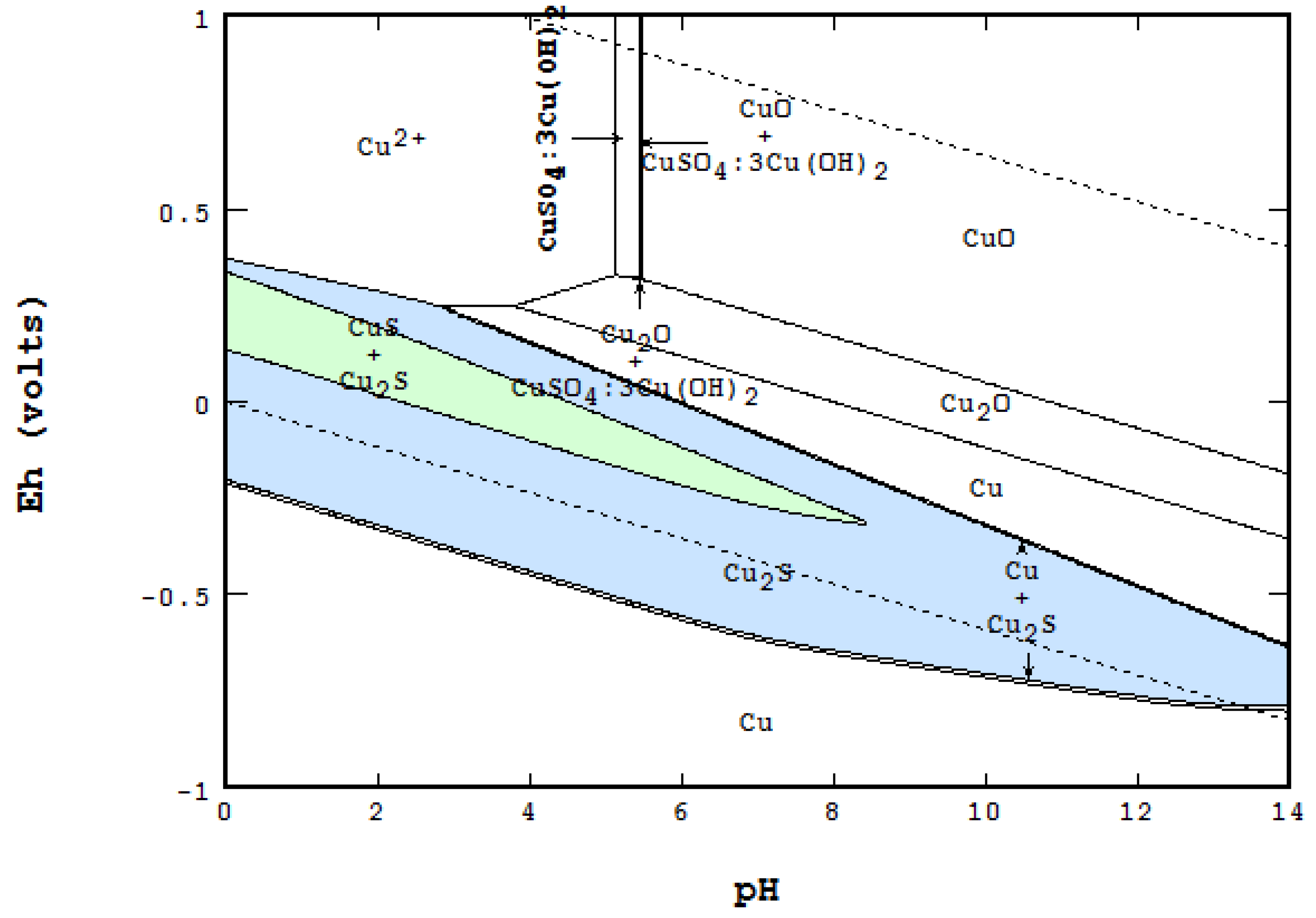
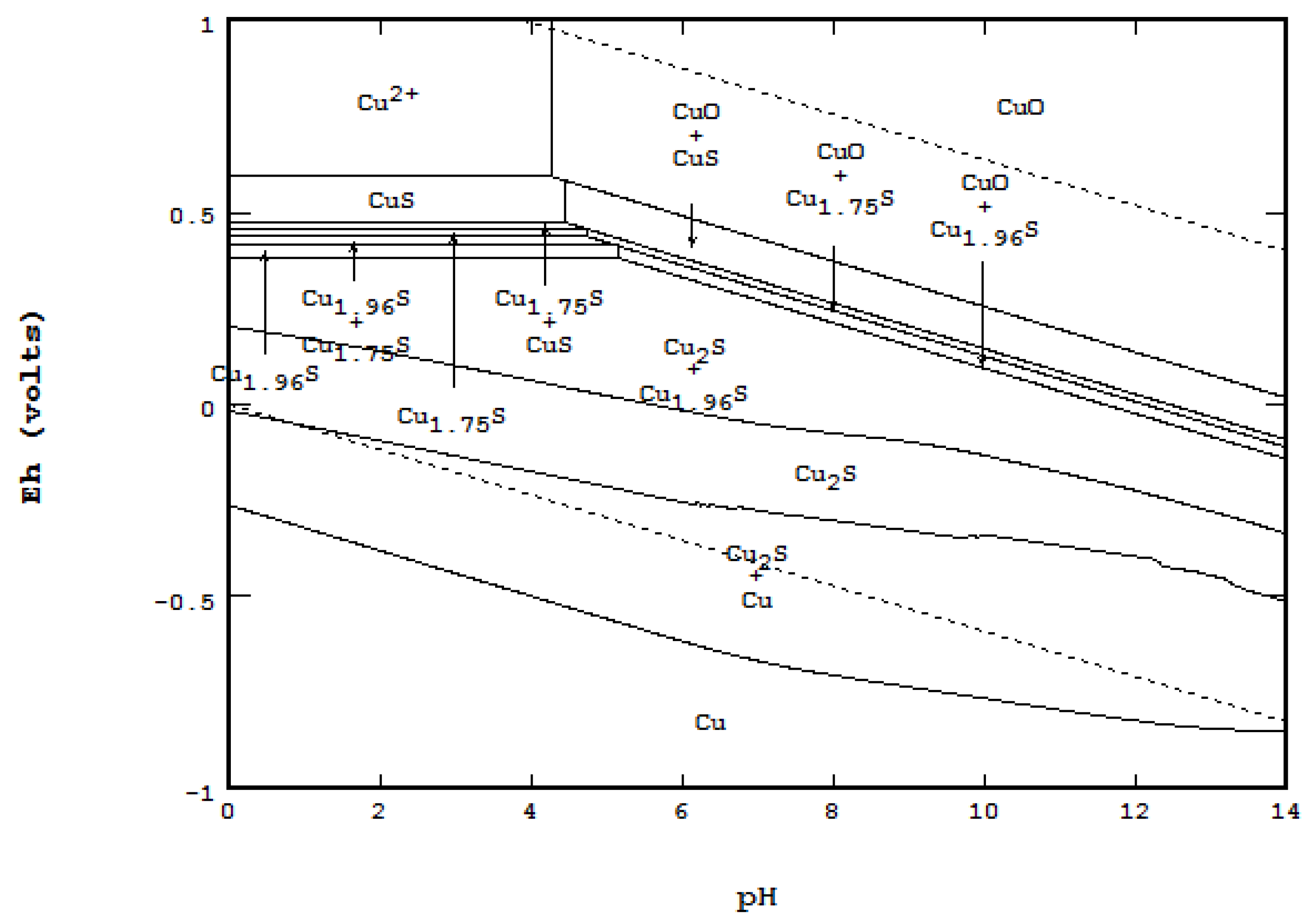
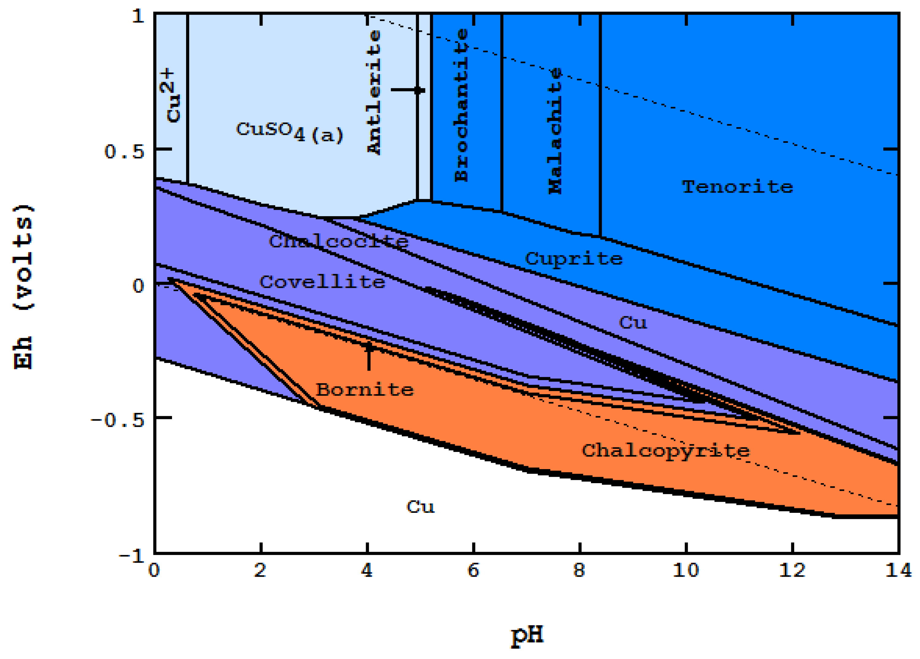
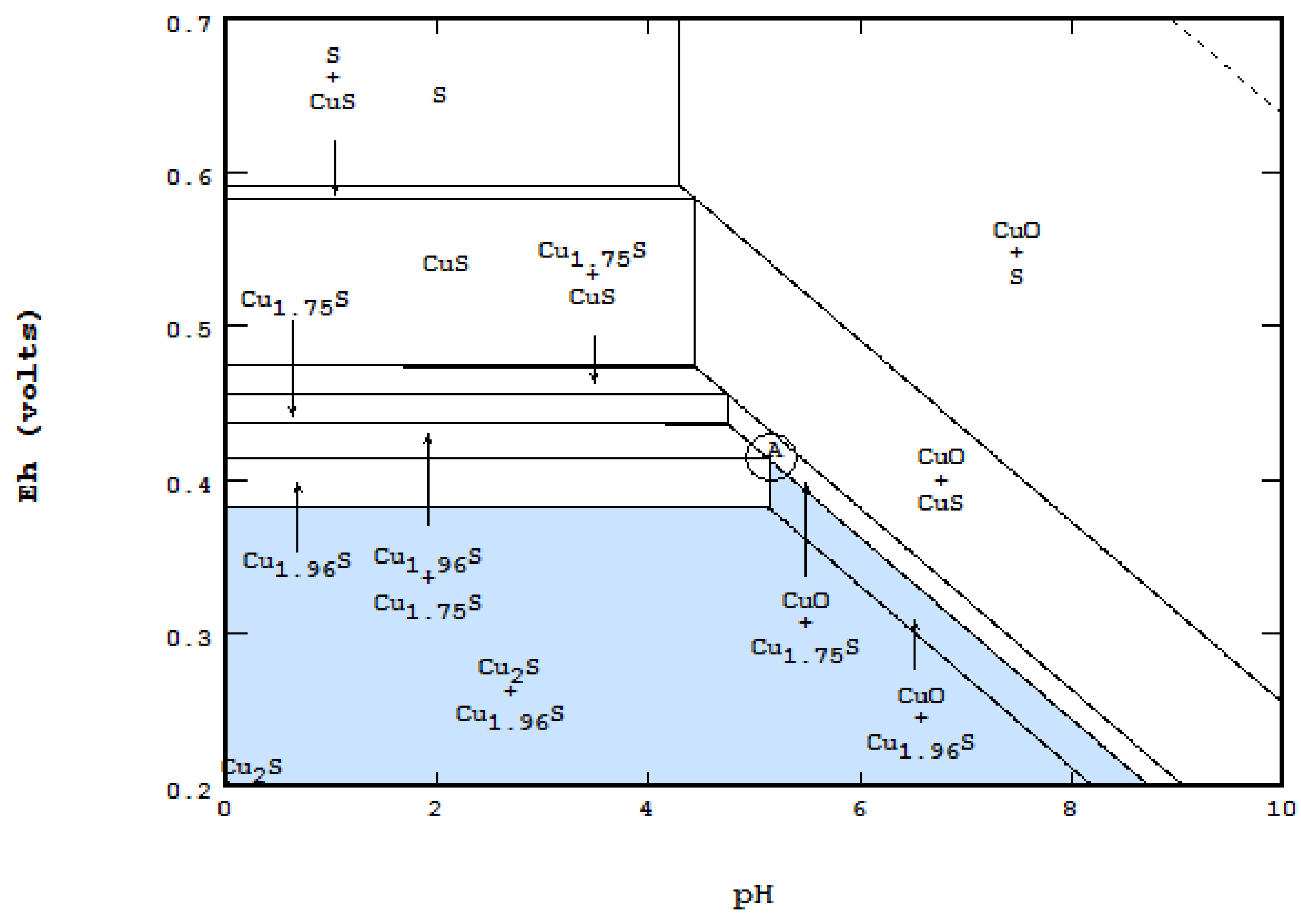
On a boundary line where F = 1, Nmaxsolid becomes three. For instance, while each of the light blue areas contains two solids, the line between them represents the presence of three: CuO, Cu2S and Cu1.96S,
1c.
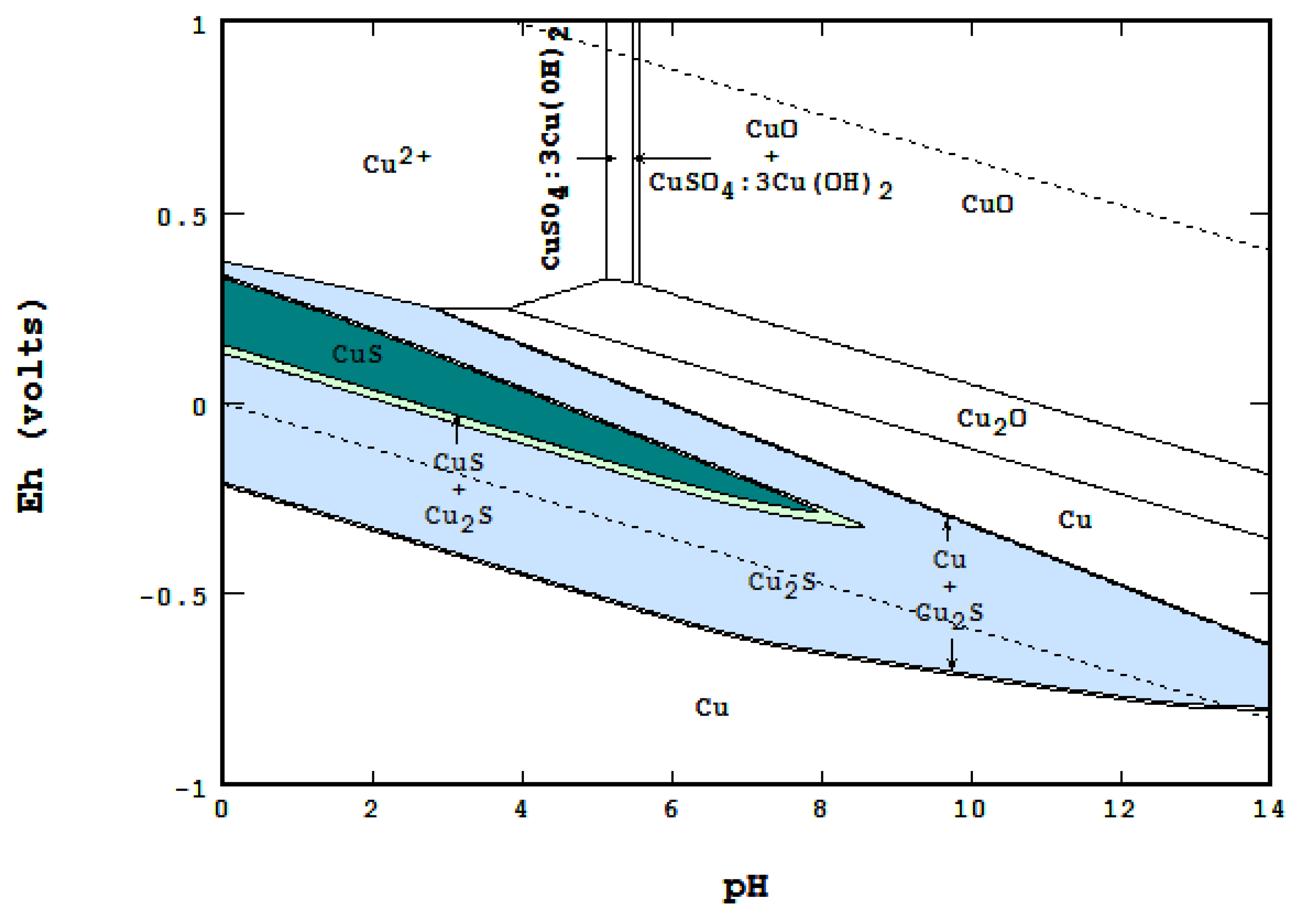
On a triple point where three lines meet, F = 0, Nmaxsolid = 4. At the point labeled A, for instance, even though four areas meet, only three solids are coexistent at the point: CuO, Cu1.75S and Cu1.96S.
Example 2, Pb-S-KEX (potassium ethyl xanthate) three-component system: Pb-S-KEX was also used to illustrate the phase rule. Figure 18 was constructed using data taken from Pritzker and Yoon [23]. The plot illustrates a small, but intricate area, Eh from −0.5 to −0.3 and pH from 10 to 13, with a resolution of 600 × 800. A small pink area shows three stable solids: PbS, Pb and PbX2. This number agrees with the phase rule equation for the Eh-pH diagram of Nmaxsolid = 5 – F, where F is equal to two, being inside an open area. There are four solids (PbS, Pb, PbX2 and Pb(OH)2) along the line between this pink area and the area right above it. The Nmaxsolid for all three corners of this area was no greater than five, as described by the rule.
Figure 17. Mass-balanced Eh-pH diagram of the Cu–S–water system to illustrate the phase rule. This is a zoomed-in detail from Figure 14; stable solids include elemental S from the S component. ΣCu = 0.118 and ΣS = 0.059 M.
Metals 06 00023 g017
Figure 18. Mass-balanced Eh-pH diagram of the Pb–S–potassium ethyl xanthate (KEX) water system. ΣPb = ΣS = 0.45 and ΣX = 0.0001 M. This zoomed-in detail has a resolution of 600 × 800 to verify the Gibbs phase rule.
Metals 06 00023 g018
Equilibrium line method: Since this method works on one component at a time, Nmaxsolid = 4 – F – 1 = 3 – F. Referring to Figure 13, in any open area of the diagram, Nmaxsolid = 1, which means only one solid is allowed. On any boundary line, Nmaxsolid = 2, as shown by the line between CuO and CuS. If a triple point is formed, Nmaxsolid will be equal to three.

5. Enhancing the Eh-pH Plot by Merging Two or More Diagrams

Most Eh-pH diagrams indicate the stability of water by two dashed lines: this is a typical example of merging two diagrams together. Other examples include showing several solubilities of solid species (see Figure 9), showing dissolved species in areas dominated by solids and showing ligands in addition to the main component (see Figure 10).
An Eh-pH diagram, including the examples listed above, often shows only half of a reaction. To illustrate the whole process, merging another relevant diagram may be necessary. The combined diagram can be re-plotted or overlaid by a graphics program, such as MS PowerPoint. It is strongly suggested to use different colors for each merged diagram.

5.1. Cyanidation of Gold and Cementation with Zn Metal

The combination of a Au–CN diagram with a Zn–CN diagram is shown as Figure 19. The up-arrow indicates leaching of Au using CN as the complexing ligand and O2 as the oxidant. The down-arrow indicates the cementation of Au replaced by Zn metal.

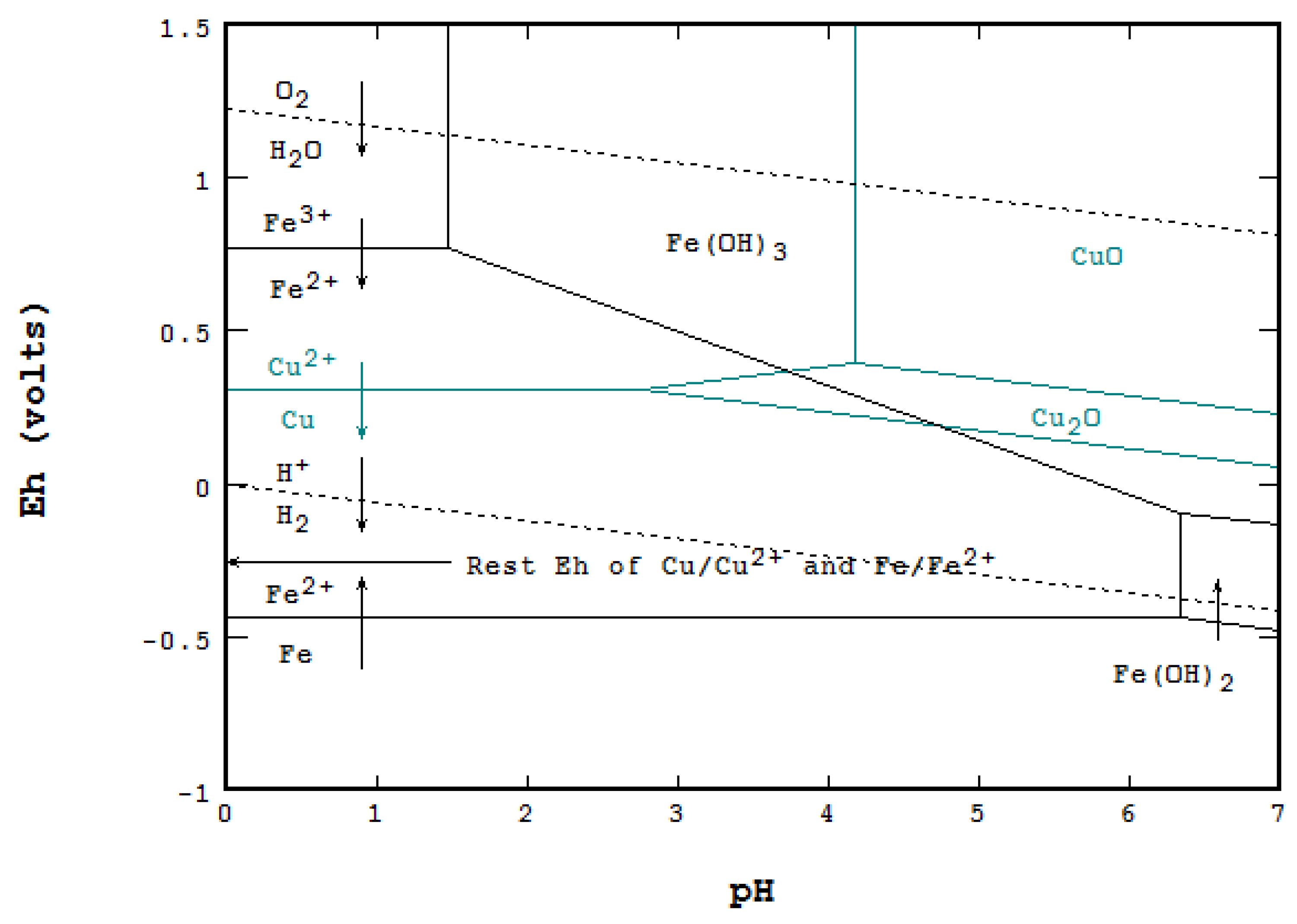
5.2. Cementation of Copper with Metallic Iron

Figure 20 shows the combination of a Cu–water diagram and a Fe-water diagram and illustrates cementation of copper by iron metal. Additionally, the diagram shows other reactions of interest, such as those that represent wasteful consumption of iron metal by reactions involving Fe3+, O2(g) and H+(a). Although not part of the diagram calculations, the rest potential between the Cu2+/Cu–Fe2+/Fe electrodes is also shown.
Figure 19. Combined Au–CN and Zn–CN Eh-pH diagrams would show leaching and cementation for the gold cyanidation process.
Metals 06 00023 g019
Figure 20. Combined Cu and Fe Eh-pH diagrams would show that reactions occur during copper cementation using metallic iron.
Metals 06 00023 g020

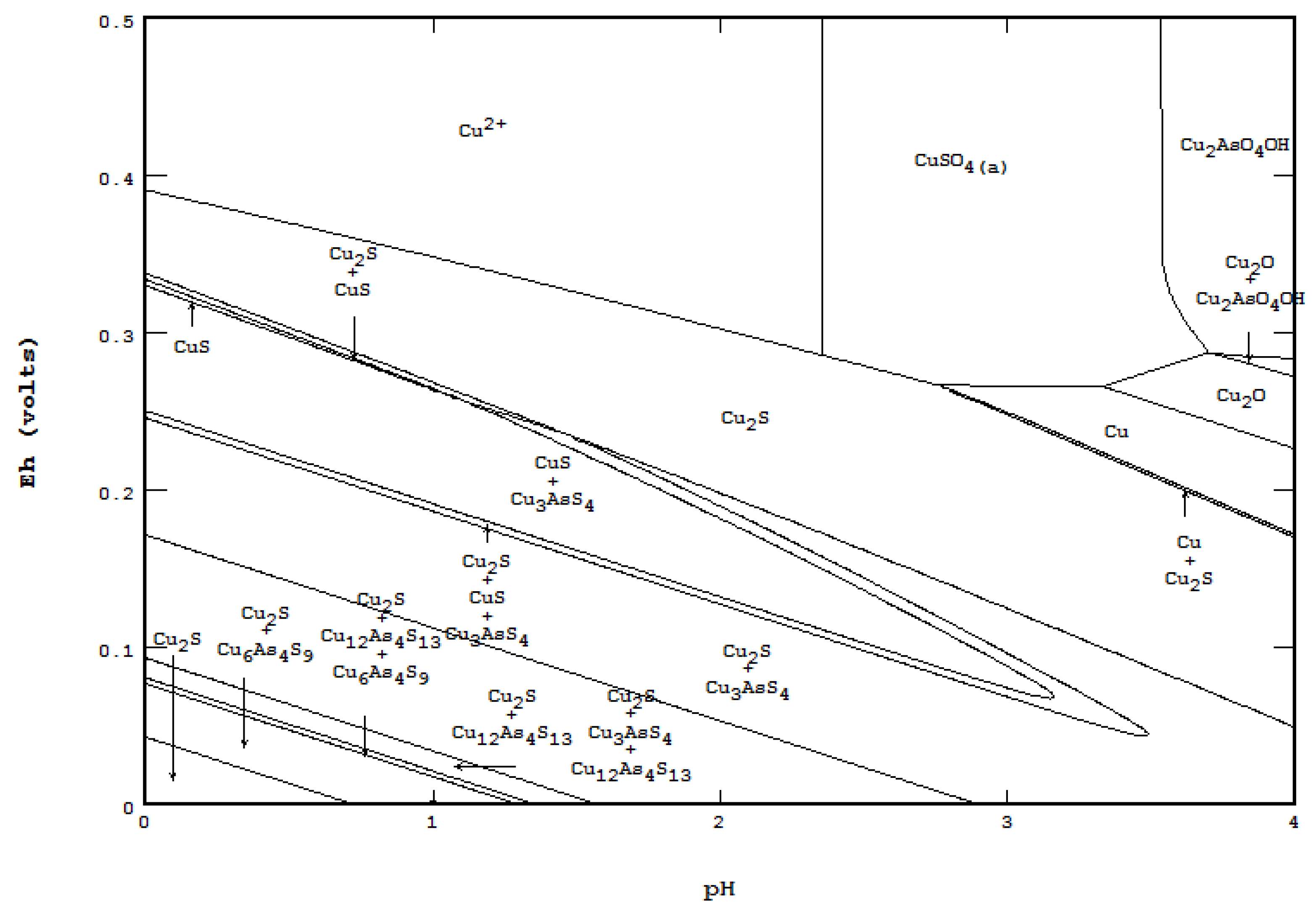
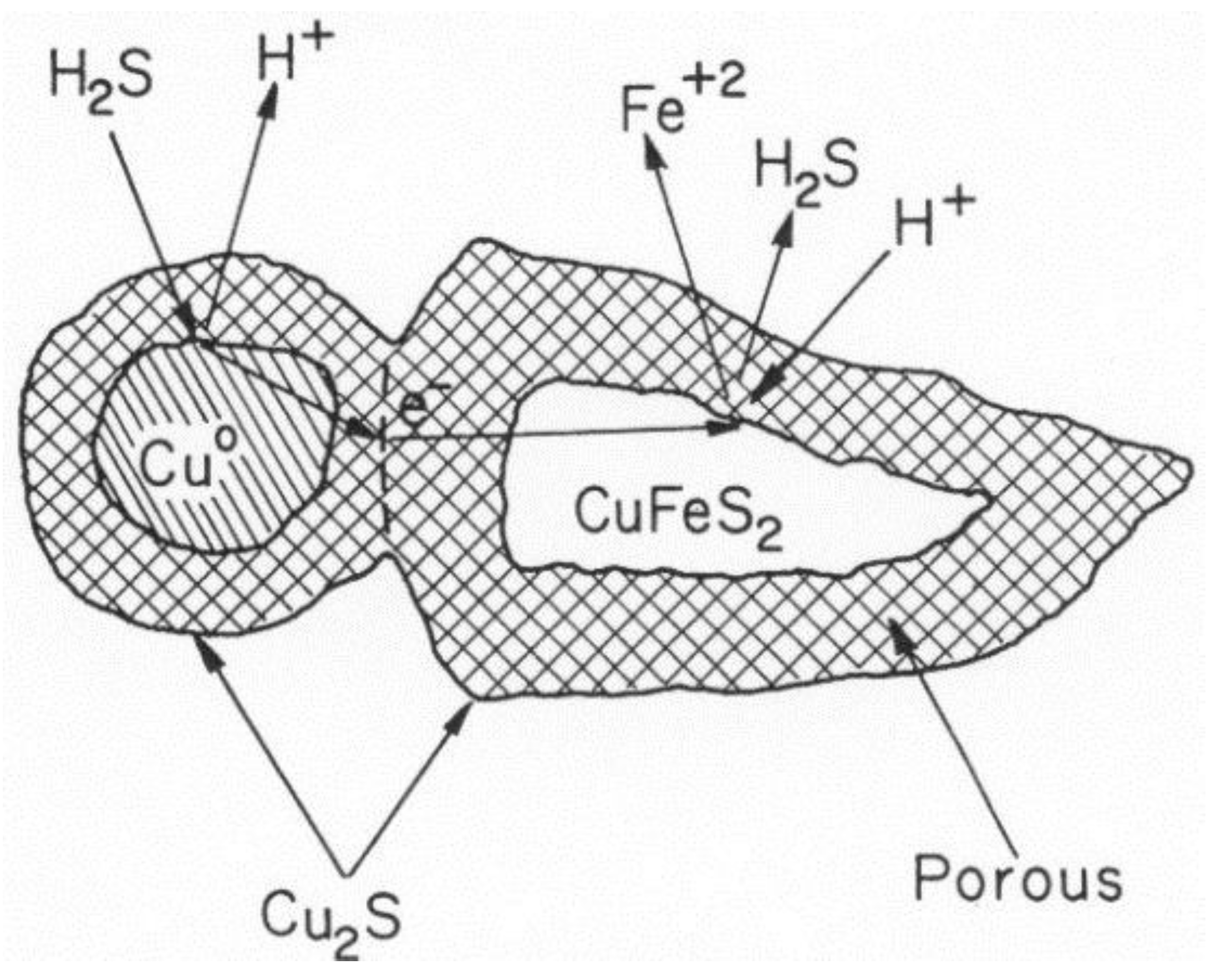
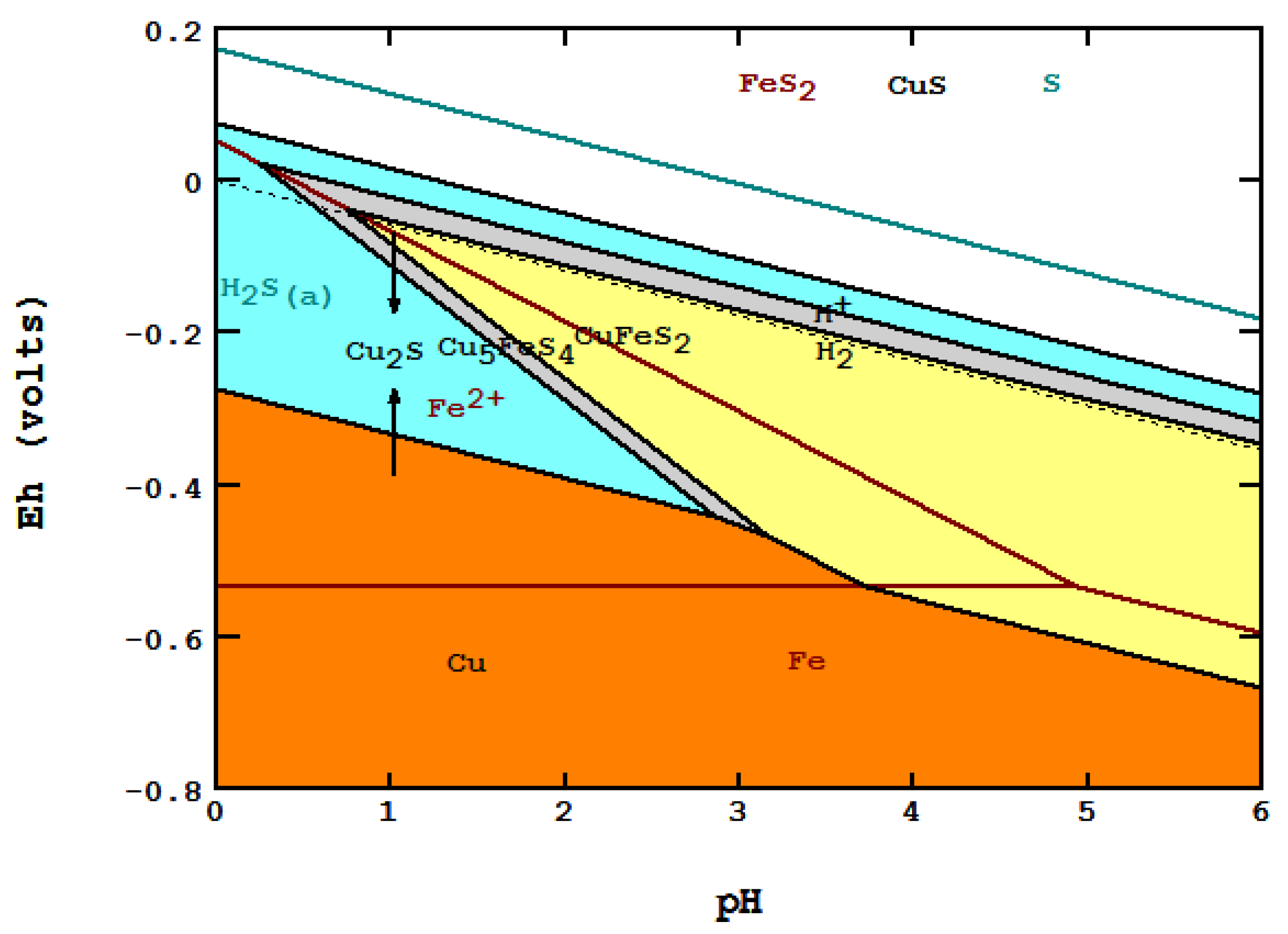
5.3. Galvanic Conversion of Chalcopyrite with Copper Metal [24]

When in contact with Cu metal, chalcopyrite reacts cathodically in an effect known as galvanic conversion:
10CuFeS2 (chalcopyrite) + 24H+ + 8e = 2Cu5FeS4 + 8Fe2+ + 12H2S
2Cu5FeS4 (bornite) + 6H+ + 2e = 5Cu2S + 2Fe2+ + 3H2S
An anodic reaction takes place on the metallic copper as:
2Cu + H2S = Cu2S + 2H+ +2e
A schematic diagram for all these reactions is shown as Figure 21. In order to present all of the species involved, three Eh-pH diagrams are superimposed and shown as Figure 22.
  • The three diagrams used are: S species in cyan, Fe and Fe–S in red and Cu–Fe–S in black.
  • Areas of predominance are shown as: chalcopyrite in yellow, bornite in gray, chalcocite in light blue and metallic copper in orange.
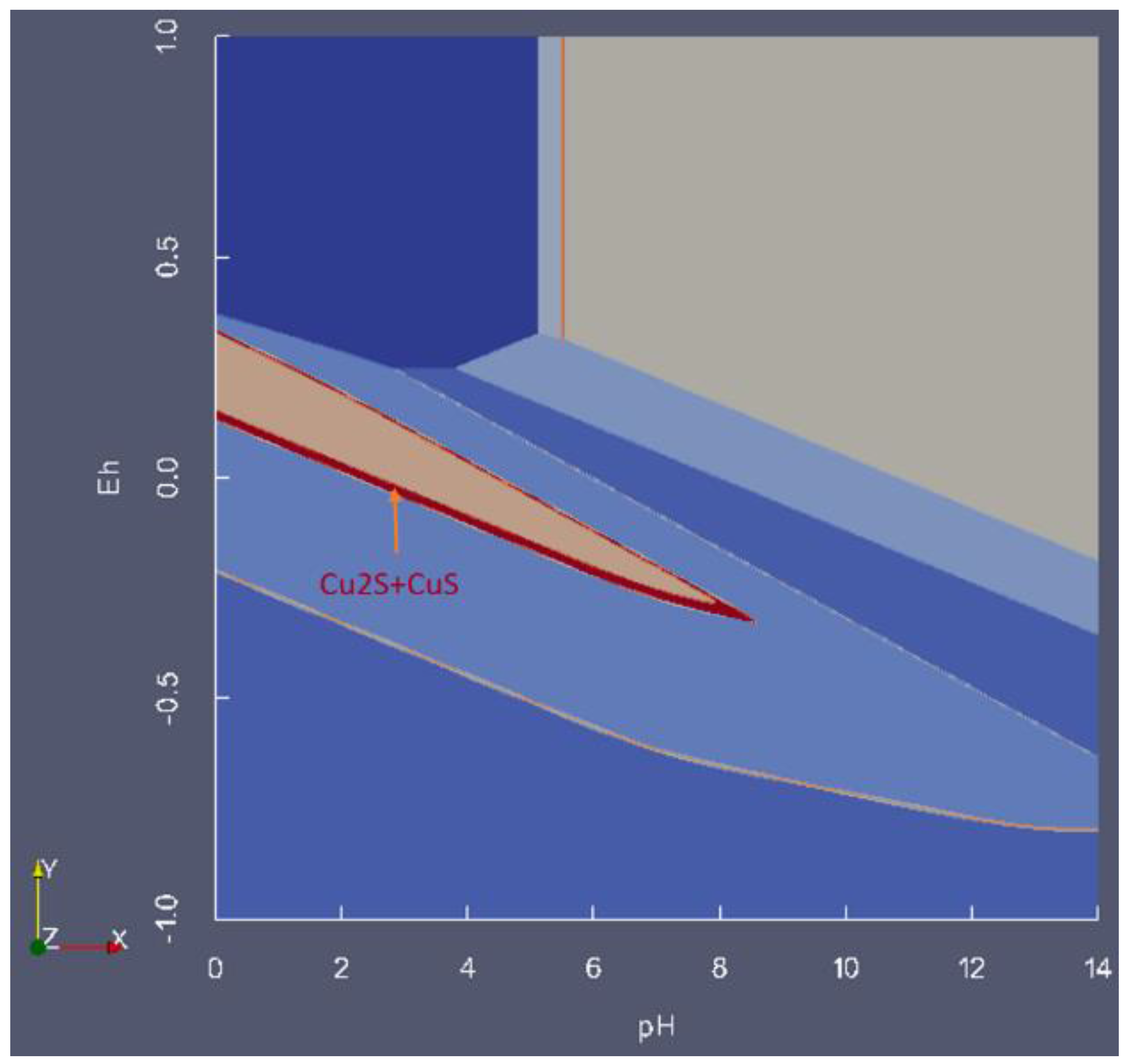
  • The down-arrow indicates where galvanic conversion occurs down from chalcopyrite to bornite and, finally, to Cu2S. The up-arrow indicates where the anodic reaction occurs up from metallic copper to Cu2S.
  • The diagram indicates that both cathodic and anodic reactions lead to the formation of Cu2S, and other final species match what Hiskey and Wadsworth [24] described.
Figure 21. Schematic diagram of reactions occurring upon galvanic conversion of chalcopyrite with metallic copper [24].
Metals 06 00023 g021
Figure 22. Combination of three Eh-pH diagrams showing the galvanic conversion reactions of chalcopyrite with metallic copper.
Metals 06 00023 g022

6. Third Dimension to an Eh-pH Diagram

Even more information may be shown by adding a third dimension to a base Eh-pH diagram. The third dimension can be the simple solubility of solid or an independent variable, such as temperature or ligand concentration. First, the data needed for a 3D Eh-pH diagram must be calculated. Thereafter, 3D programs for PC, such as ParaView [25], VisIt [26] or MATLAB [27], combine all of the data into a single diagram. These programs can also provide other functions, such as animated rotation, clipping and slicing. This section presents some 3D examples by considering extension of the Eh-pH diagram into a third dimension. Data creation and setup input files for a 3D program are briefly presented. Three areas are illustrated:
  • Eh-pH along with the solubility of stable solids; two example diagrams are illustrated: passivation of lead (Figure 6) and adsorption of As(III) and As(V) onto ferrihydrite (Figure 8).
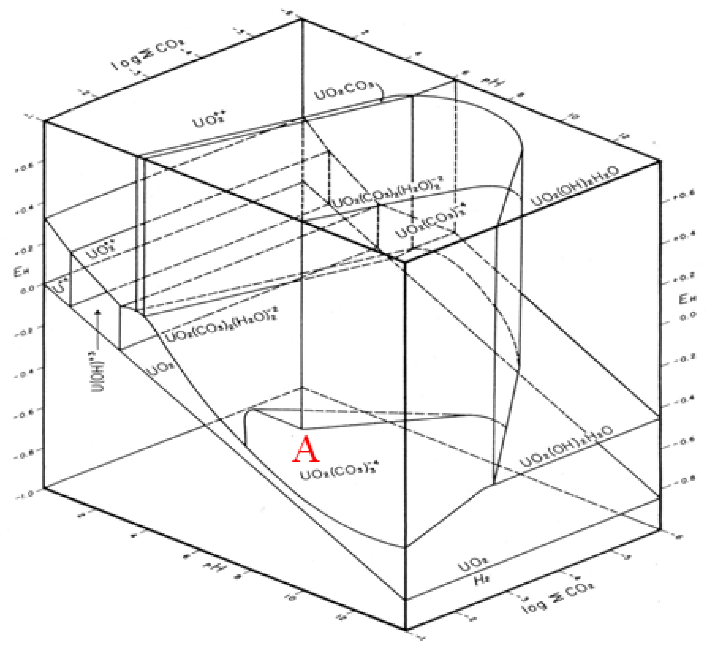
  • Eh-pH with an extra axis for ligand CO2: two wireframe volume diagrams of Eh-pH-CO2 taken from Garrels and Christ [2] are used for verifying the results; these two are:
    • Figure 7.32b: in order to match the given ΣCO2 for the third axis, the mass balance method has to be used; the output of 3D and discussion for this case are presented in more detail.
    • Figure 7.32a: since the third axis is given as the pressure of CO2(g), the equilibrium line method can be applied; the time required for the Eh-pH calculation was much less.
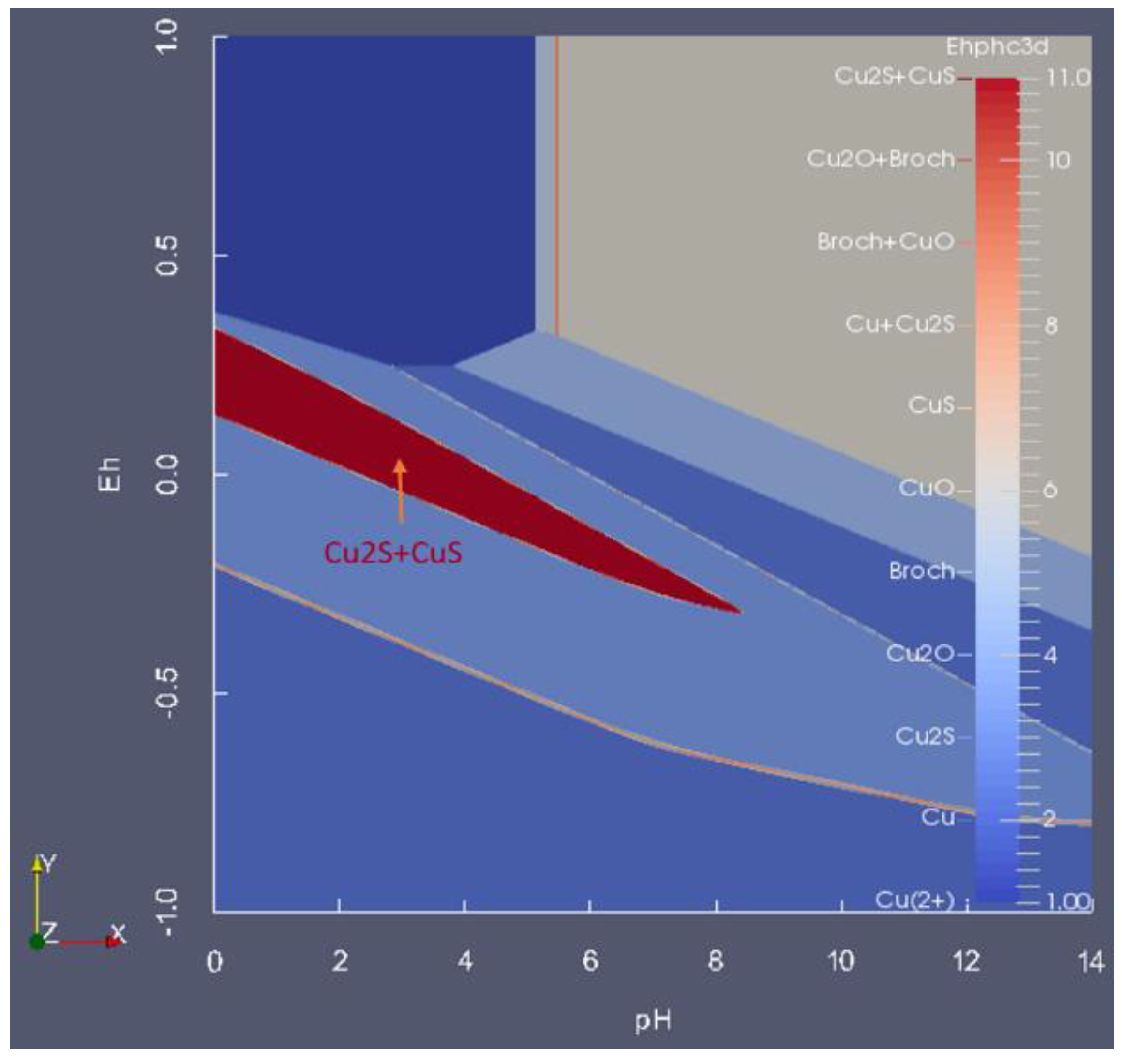
  • Presentation of a system in which two or more solid phases, such as CuS and Cu2S, can coexist.

6.1. Eh-pH with Solubility

Including the solubility of solids in an Eh-pH diagram can give a much clearer view of what can happen to the solid. The following two diagrams constructed by MATLAB extend the 2D Eh-pH diagrams presented earlier. In order for MATLAB to plot 3D solubility diagrams, the Eh-pH program needs to create two files: the (name).m file contains instructions to be executed by MATLAB, and the data file contains solubility from each Eh and pH from the grid. A MATLAB plot can show the matching contour (iso-solubility) lines below the 3D feature.
Figure 23 is an extension of Figure 6, showing the solubility of Pb(II) as the third dimension. The red areas indicate conditions where corrosion can be expected to occur. The gulch area in yellow indicates conditions where Pb(II) is passivated by CO2.
Figure 23. The Eh-pH plus solubility diagram for Pb–CO3–water. The yellow gulch area in the middle is where Pb(II) is likely passivated by CO3.
Metals 06 00023 g023
Figure 24 illustrates the same system as Figure 8, which showed where As(V) and (III) can be adsorbed upon the formation of ferrihydrite. The solubility diagram shows where the lowest concentrations of As(V) and (III) can be achieved. The deep blue area at the low Eh of the diagram is where arsenic metal becomes stable and immunized from corrosion.
Figure 24. The Eh-pH plus solubility diagram for As–Fe–water. The valley area on the left is where the greatest adsorption of arsenic can occur.
Metals 06 00023 g024

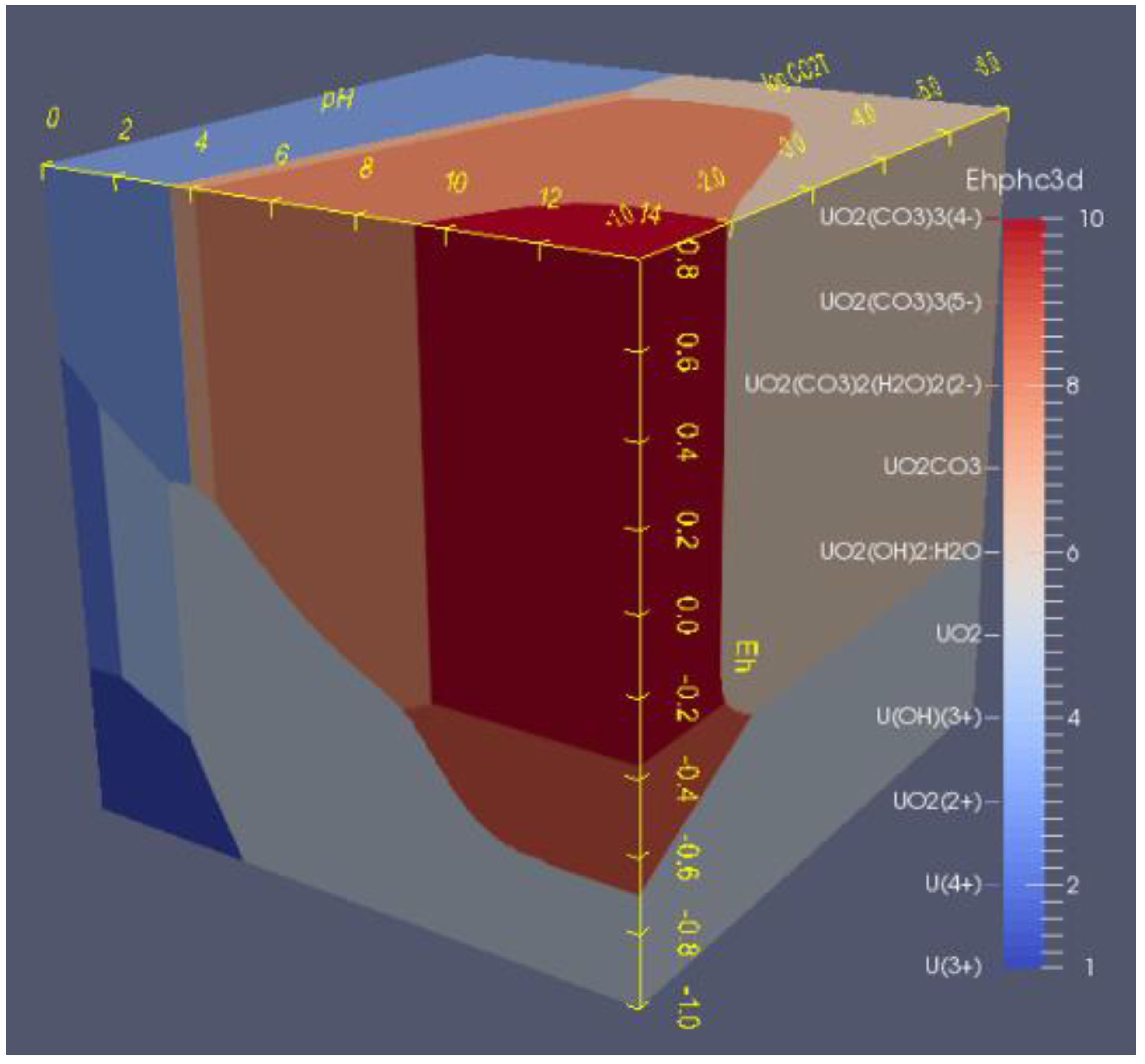
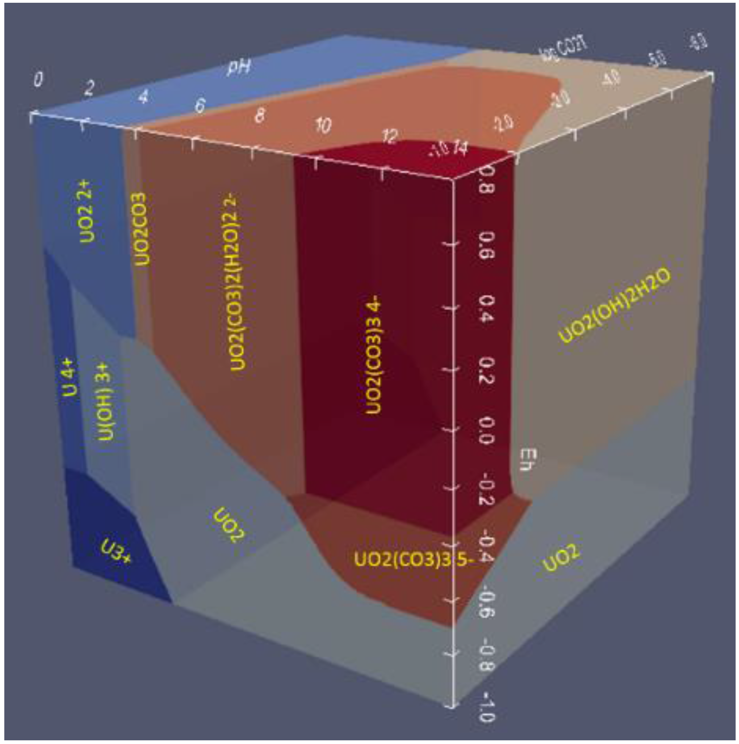
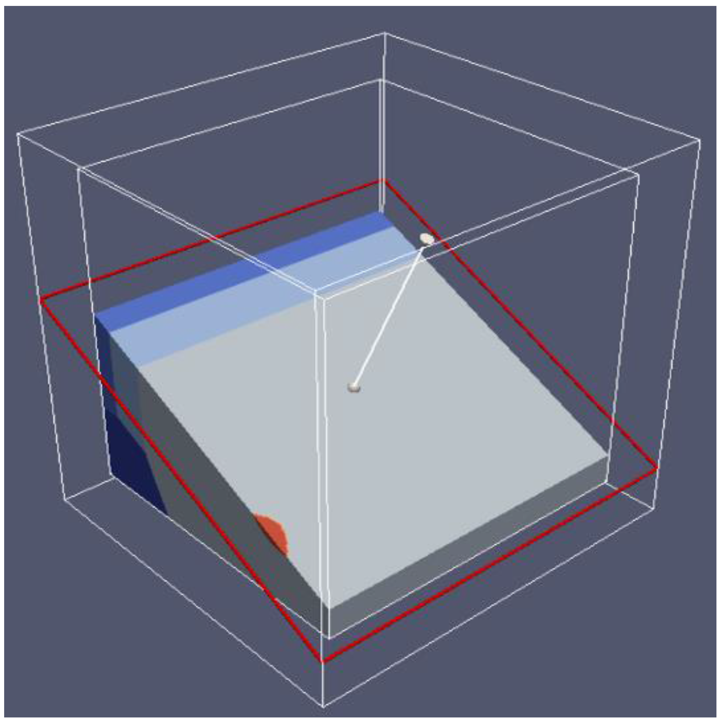
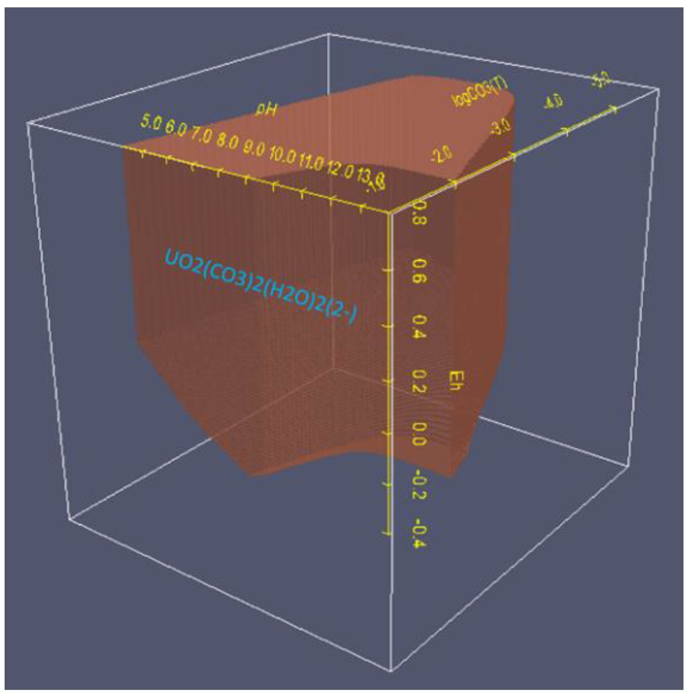
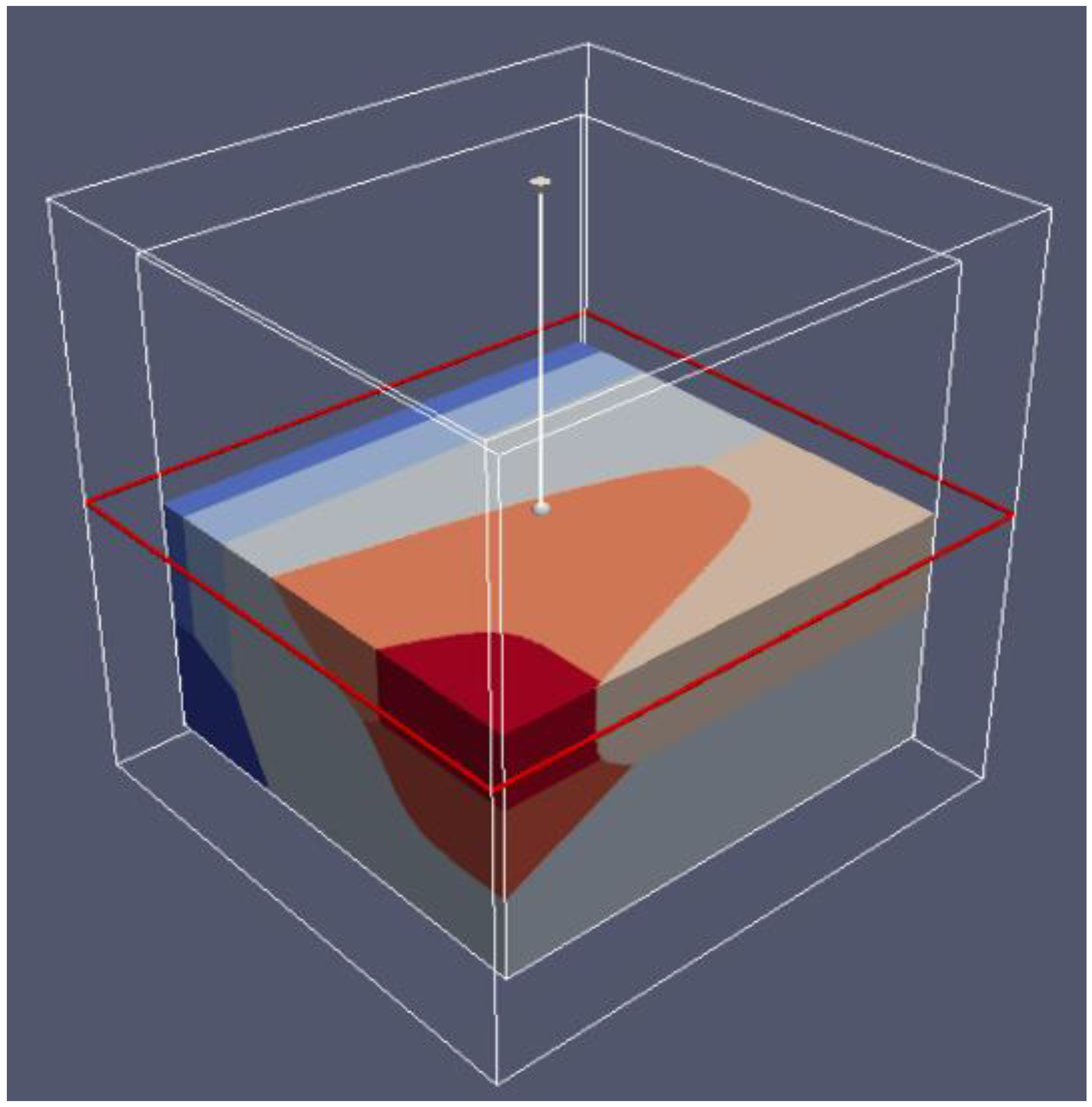
6.2. 3D Eh-pH, Uranium with ΣCO2: Using the Mass-Balance Point Method

Example system: Figure 7.23b from Garrels and Christ [2] is one of the earliest three-dimensional diagrams for the U–CO2–water system. It is an Eh-pH diagram with the concentration of CO2 used for the third dimension. See the duplicated plot from Figure 25. In it, each predominant species is enclosed by the faces of adjacent species. A semi-transparency presentation can be a more advanced graphical method, but it had not been developed at the time. A comparison to the Garrels and Christ plot was generated, considering the same species and their ΔG0s (Free energy of formation). Other considerations required are:
  • One species in one volume: Since total carbonate is given, assuming total CO2 means all carbonates, including dissolved, solids and complexes with U, the mass-balanced method for Eh-pH diagram is used. However, to match the Garrels and Christ plot, only one single solid in each volume was selected, with no regions of mixed solids allowed.
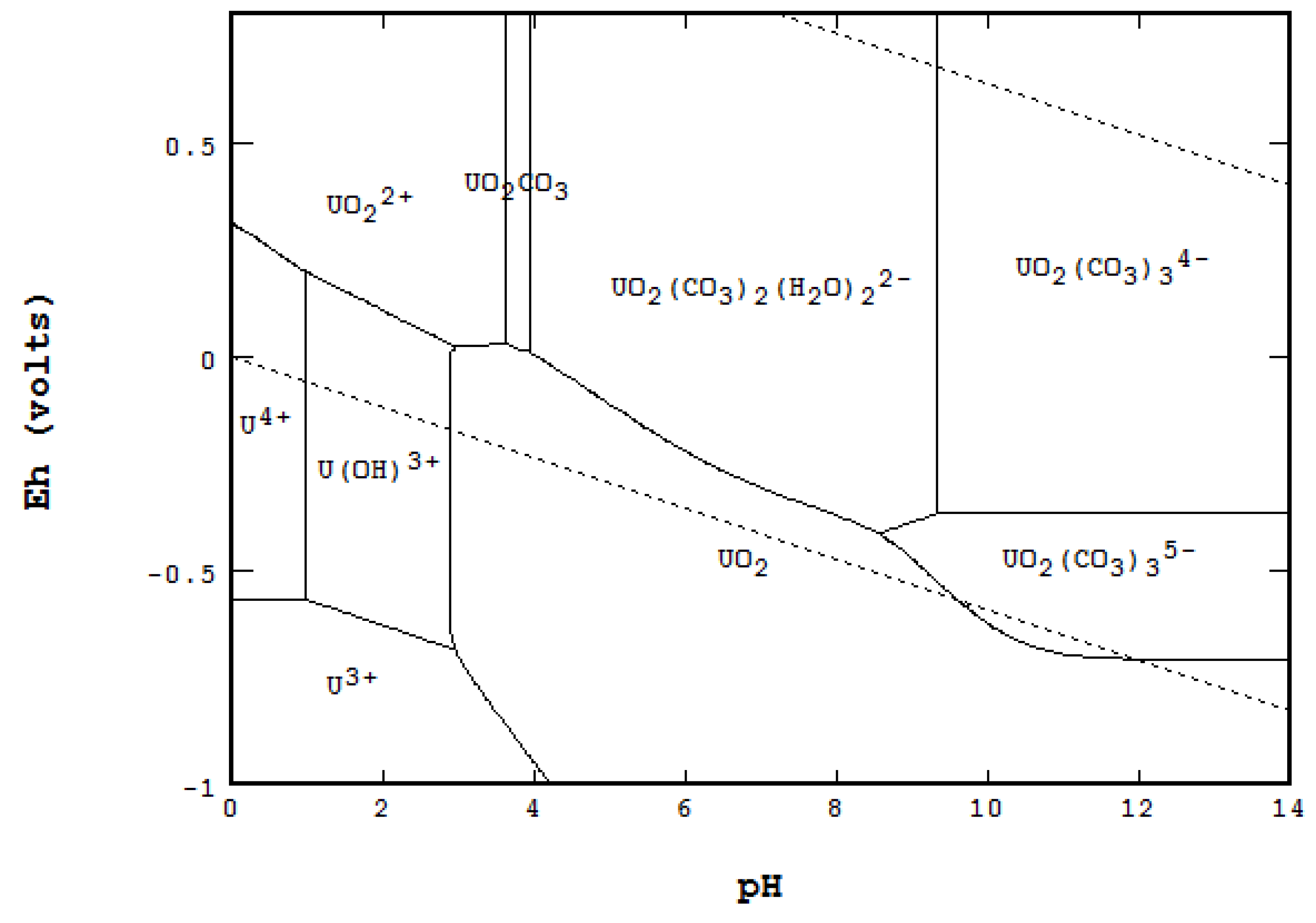
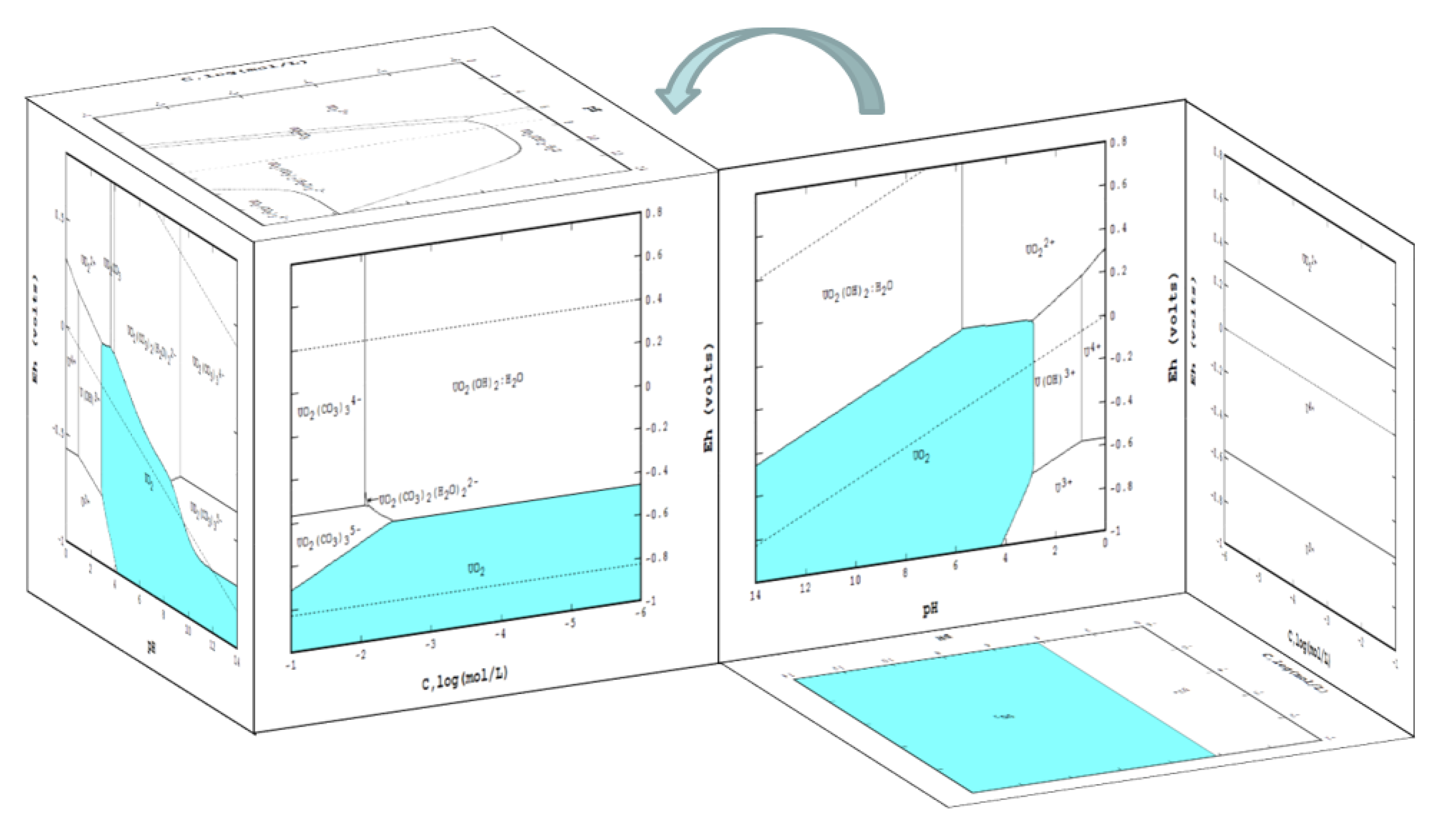
  • One missing species: One species on the Garrels and Christ diagram, indicated by a red letter A in Figure 25, seems to have been mislabeled as UO2(CO3)4−. Judging from its high pH and carbonate location, and being sandwiched between U(IV) and U(VI), the species UO2(CO3)35− [28] seems to be a good fit. Figure 26 is the regenerated 2D Eh-pH diagram using logΣCO2 = −1 M.
Figure 25. 3D diagram after Garrels and Christ. Label A is where the questionable species is located.
Metals 06 00023 g025
Figure 26. The Eh-pH diagram of U with logΣCO2 = −1. The inclusion of UO2(CO3)35− clarifies a region that Garrels and Christ might have misrepresented.
Metals 06 00023 g026
Example diagrams and conditions: Figure 27, Figure 28, Figure 29, Figure 30, Figure 31 and Figure 32 are three-dimensional diagrams created using ParaView (Version 4.3.1) based on the data generated by the STABCAL program. Although the complete ParaView diagram allows such functions as continuous rotation, clipping and slicing, these static diagrams demonstrate the range of features that can be achieved. A color map (bar), shown in Figure 27, indicates that the names of the species should be added at least once to one of the figures. Computational conditional limits include:
  • Ranges: Eh = −1 to 0.8, pH = 0 to 14 and logΣCO2 = −6 to −1,
  • Grid point: 250 × 250 × 250,
  • Computer: 64 bit, 3.40 GHz, 16 G of RAM,
  • Program algorithm: mass balance point method using mass action law,
  • Accuracy (sum of squared residual) <1 × 10⁻⁸ and
  • Time to complete the calculation: 1:36:25 (h:mm:ss) from i7 PC or 2:00:51 from i5; contrary to using the line method, shown later, which took less than 30 s.
In order for ParaView to plot a 3D diagram, the Eh-pH program needs to create a (name).vtk file [29] that specifies the type of grid, the values of all X, Y and Z coordinates followed by all of the point data that indicate which species are to be plotted for each point on all three axes.
Figure 27. Eh-pH-logΣCO2 of uranium where the species are shown by colors. A color bar is inserted to show the corresponding species.
Metals 06 00023 g027
Figure 28. The transparent view of the 3D plot. Each colored area is labeled with the name of the species.
Metals 06 00023 g028
Figure 29. The clip plot shows only regions below the constraint of Eh −0.1 V.
Metals 06 00023 g029
Figure 30. The clip plot shows species below the plane of theoretic water stability between H2O and H2(g). Compare to the lower dashed water line in Figure 26 or the lower plane where no species were shown in Figure 25.
Metals 06 00023 g030
Figure 31. 3D plot that shows the boundaries (contour) between species.
Metals 06 00023 g031
Figure 32. Semi-transparent plot that shows the stability region of UO2(CO3)2(H2O)22− species.
Metals 06 00023 g032
A three-dimensional plot has the great advantage of being able to show the effects of multiple variables at once. Tools, such as rotate, slice and clip, can easily identify areas of particular interest. For a complicated system, however, a three-dimensional image may not be as clear as a two-dimensional drawing due to the memory and screen resolution imposed by an ordinary PC. It is therefore wise to choose or combine the use of 2D and 3D to have the best presentation.
A simple way to turn a set of line-drawn diagrams into a three-dimensional object is to arrange six two-dimensional surface plots (two from each of Eh-pH, Eh-ligand and pH-ligand) into a cube. It may be necessary to reverse the x- or y-axis direction for this purpose. Simple plastic cubes, intended for use with photographs, are readily available. See Figure 33, where the section on the left (three plots combined) is the top-front view and the section on the right is the bottom-rear view. The two sections are jointed along the Eh axis, at pH = 14 and log ΣCO3 = −1 M. Rotating the right sections to the left will make a complete cube. To show the continuity between plots, species UO2 was purposely colored in light blue.
Figure 33. Combination of six surface plots of the U Eh-pH-logΣCO2 system to form a cube.
Metals 06 00023 g033

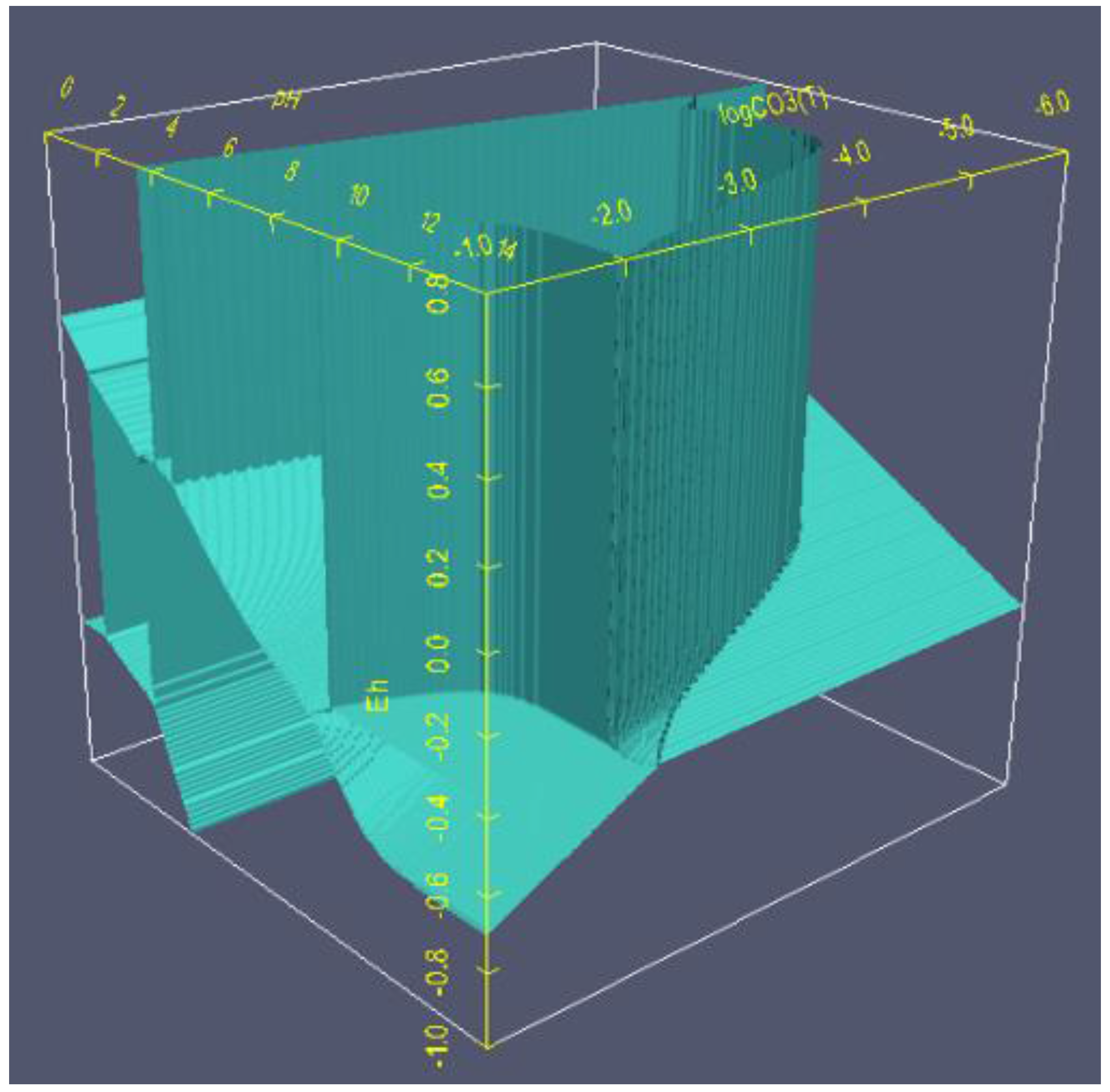
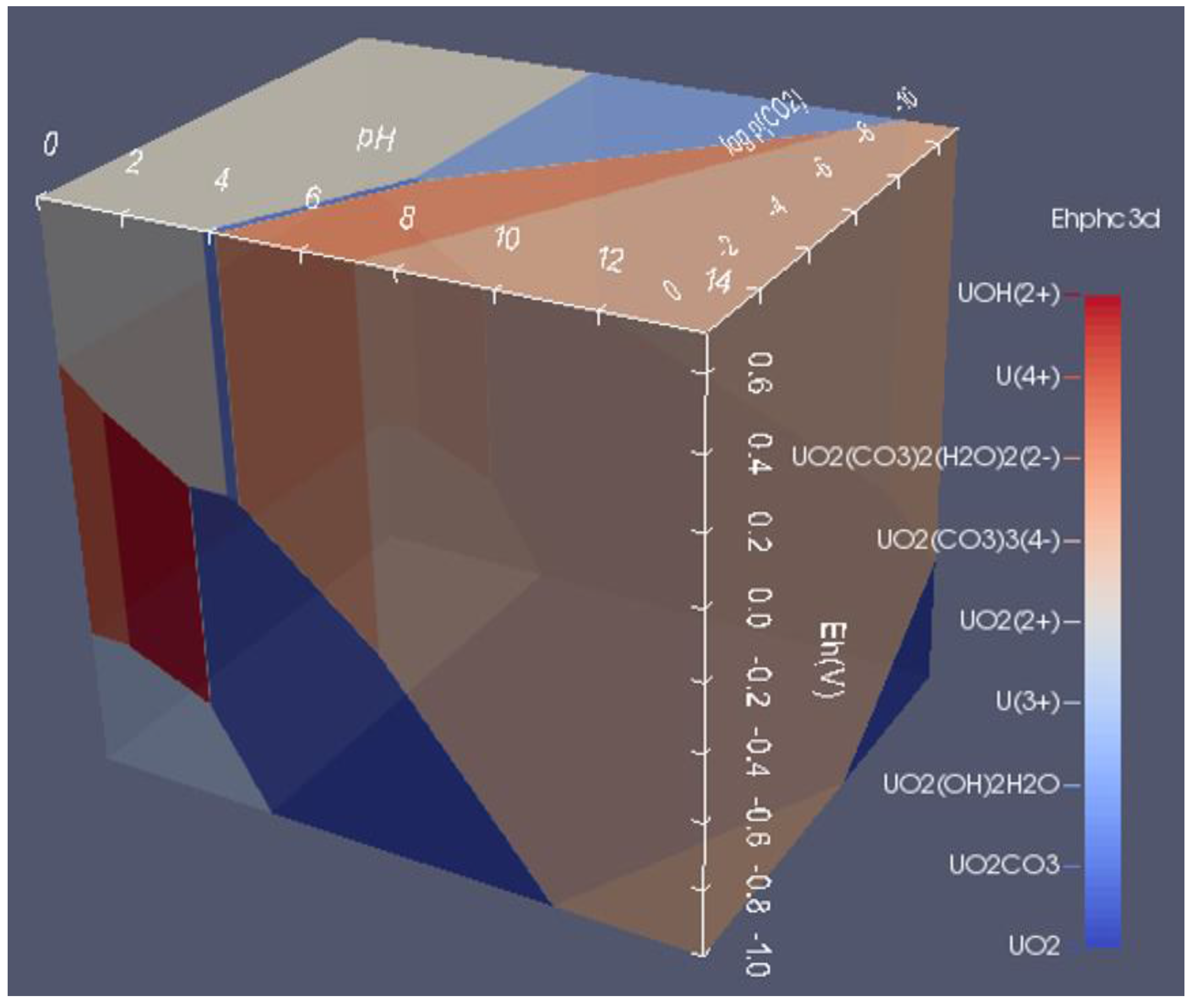
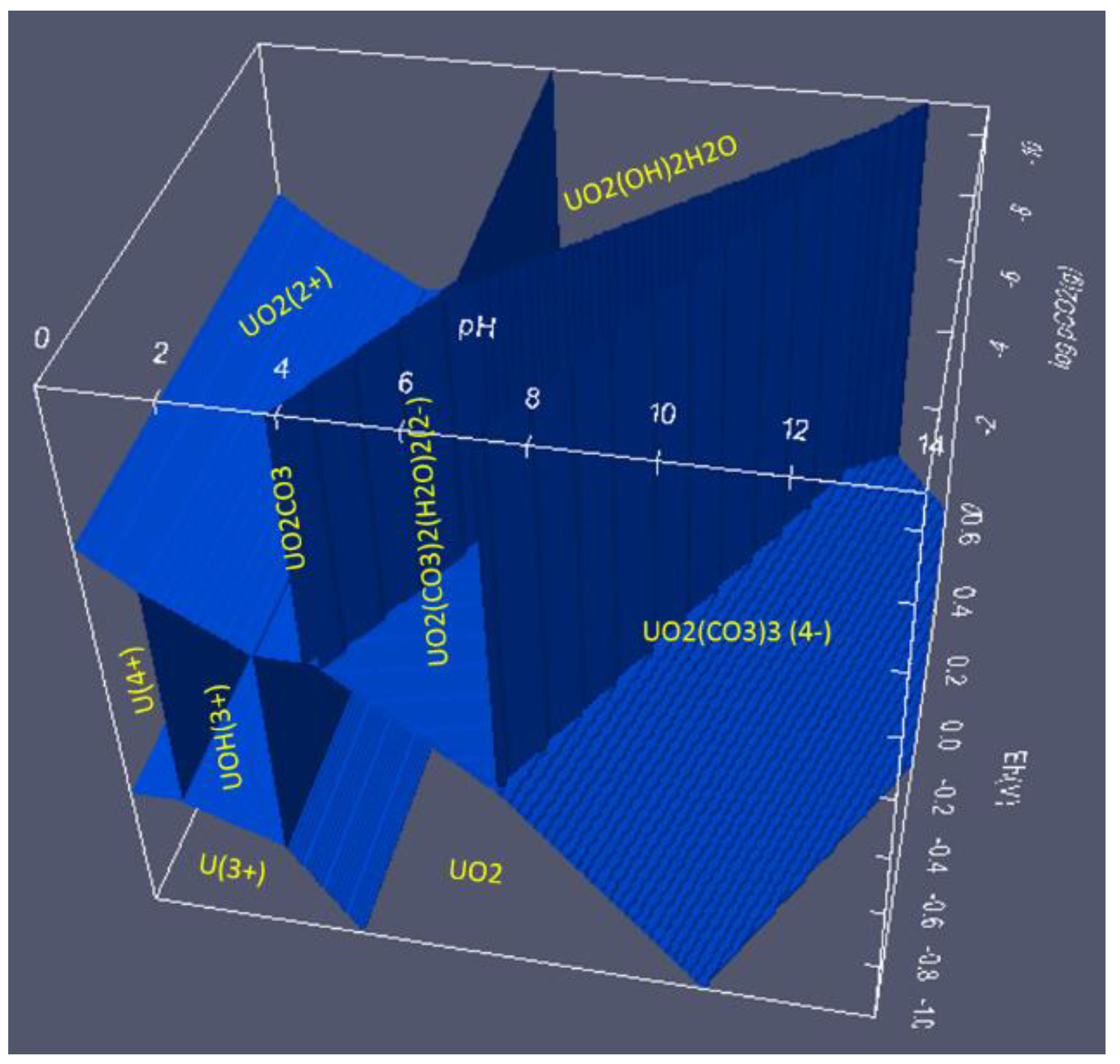
6.3. 3D Eh-pH, Uranium with Pressure CO2(g): Using the Equilibrium Line Method

This example used Figure 7.32a from Garrels and Christ for U with the CO2 system. Since the extra axis is the pressure of CO2(g), the equilibrium line method was used. The Eh-pH program took less than 30 s to create necessary data for making the (name).vtk file for ParaView. Without having to repeat the same features presented earlier, only the semi-transparent surfaces and the boundaries between species are shown on Figure 34 and Figure 35, respectively. These two plots agree with the original diagram presented by Garrels and Christ.
Figure 34. Eh-pH-logpCO2(g) of uranium where the species are shown by colors. This diagram matches Figure 7.32a of Garrels and Christ.
Metals 06 00023 g034
Figure 35. 3D plot that shows the boundaries (contour) between species. This diagram used data from the line method where logpCO2(g) was given.
Metals 06 00023 g035

6.4. How to Show Two or More Solids in One Area

ParaView is capable of showing areas occupied by more than one solid phase. As with single solid regions, multi-phase areas are also colored and shown on the color map. Using the same conditions as for Figure 11 and Figure 12, Figure 36 and Figure 37 are plotted by ParaView indicating four two-solid phases. The areas occupied by CuS plus Cu2S are indicated in red and pointed to by an arrow.
Figure 36. ParaView of Cu–S–water, where ΣCu = 0.001 and ΣS = 0.0009 M. See the 2D plot of Figure 11 for a comparison.
Metals 06 00023 g036
Figure 37. ParaView of Cu–S–water, where ΣCu = 0.001 and ΣS = 0.0011 M. See the 2D plot of Figure 12 for a comparison.
Metals 06 00023 g037

7. Summary

An Eh-pH diagram, commonly known as a Pourbaix diagram, is an effective way of presenting the effects from oxidation-reduction potential, acid and base, complexing ligands, temperature and pressure for an aqueous system. It can be used in many scientific fields, including hydro- and electro-metallurgy, geo and solution chemistry and corrosion science. Diagrams describing natural copper deposits, lead corrosion prevention and arsenic adsorption by ferrihydrite and leaching and metal recovery were illustrated. The fundamental principles behind the diagram were briefly described.
To handle ligand components for these diagrams, two separate methods developed over time, the line of equilibrium concentration and the point of complete mass balances, were described and illustrated. Both satisfy the Gibbs phase rule in their own way of calculation. The comparison and applications from these two methods are mentioned and illustrated.
Many advances of the Eh-pH diagrams are presented. These are:
Merging diagrams: Most of the Eh-pH diagrams describe only half of the reactions. Merging several same-sized Eh-pH diagrams together can better illustrate the overall system. Examples include cyanidation of Au plus cementation with Zn metal, cementation of Cu with metallic Fe and galvanic conversion of chalcopyrite with metallic Cu.
Creating 3D diagrams: Expanding the Eh-pH program to create data from an extra axis is relatively simple. However, a more professional third party 3D program is the best choice for drawing the final diagram. The author has tested ParaView, VisIt and MATLAB for 3D Eh-pH diagrams. Most of these programs can perform animations, such as rotation, clipping and slicing. The diagram can be semi-transparent or show the boundary for better illustration. The following examples are demonstrated:
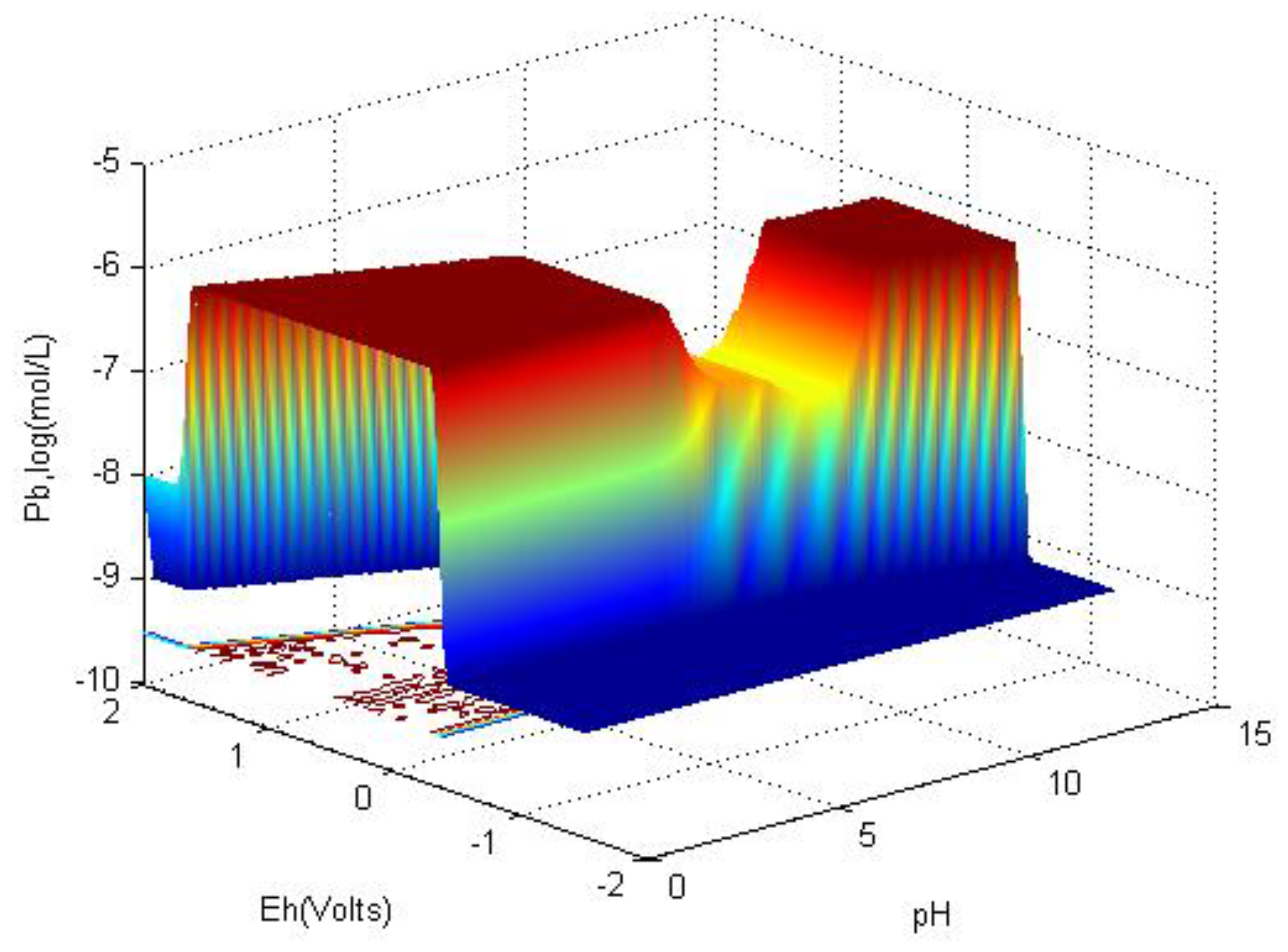
  • An Eh-pH diagram that shows solubility. Examples include: lead corrosion prevention with CO2 and concentrations of arsenic adsorption by ferrihydrite; MATLAB was used for more colorful pictures.
  • An Eh-pH with an independent variable; diagrams created by ParaView were illustrated for its functionality, and example are:
    • The mass balance point method for the Uranium system where the extra axis is log(ΣCO3);
    • The equilibrium line method for the Uranium system where the third axis is logp(CO2(g));
    • The Cu–S system for showing the coexistence of two or more solids in one volume.
When a 3D picture becomes too complex to label all of the species involved, two-variable diagrams (Eh-pH, Eh-ligand, Eh-temperature or pH-ligand) can be presented side-by-side for clarity.

Acknowledgments

The author would like to thank Dave Tahija, Hecla Greens Creek Mining, for editing this manuscript and Chen-Luh Lin, Metallurgical Engineering University of Utah, for introducing the use of ParaView. Thanks to colleagues in the Department of Metallurgical and Materials Engineering at Montana Tech for their support, in particular Courtney A. Young, Chairman of the Department, for introducing the mass balance method and encouragement for continuing development of the STABCAL program, and to Steve McGrath for his valuable discussion on the 3D Uranium-carbonate diagrams from Garrels and Christ.

Conflicts of Interest

The author declares no conflict of interest.

References

  1. Wagman, D.D.; Evans, W.H.; Parker, V.B.; Schumm, R.H.; Halow, I.; Bailey, S.M.; Churney, K.L.; Nuttall, R.L. The NBS tables of chemical thermodynamic properties. J. Phys. Chem. Ref. Data 1982. [Google Scholar] [CrossRef]
  2. Garrels, R.M.; Christ, C.L. Eh-pH. In Solutions, Minerals, and Equilibria; Freeman, Cooper & Company: New York, NY, USA, 1975; Chapter 7; pp. 172–277. [Google Scholar]
  3. STABCAL, version 2015; Stability Calculation for Aqueous and Nonaqueous System; Montana Tech: Butte, MT, USA, 2015.
  4. Pourbaix, M. Atlas of Electrochemical Equilibria in Aqueous Solution, 1st ed.; Pergamon Press: Bristol, UK, 1966. [Google Scholar]
  5. Huang, H.H.; Cuentas, L. Construction of Eh-pH and Other Stability Diagrams of Uranium in a Multicomponent system with a Microcomputer—I. Domains of Predominance Diagram. Can. Metall. Q. 1989, 28, 225–234. [Google Scholar] [CrossRef]
  6. Forssberg, E.; Antti, B.-M.; Palsson, B. Computer-assisted Calculations of thermodynamic equilibria in the Chalcopyrite-ethyl xanthate system. In Reagents in the Minerals Industry; Jones, M.J., Oblatt, R., Eds.; The Institution of Mining and Metallurgy: London, UK, 1984; pp. 251–264. [Google Scholar]
  7. Eriksson, G.A. An algorithm for the computation of aqueous multicomponent, multiphase equilibria. Anal. Chim. Acta 1979, 112, 375–383. [Google Scholar] [CrossRef]
  8. Woods, R.; Yoon, R.H.; Young, C.A. Eh-pH diagrams for stable and metastable phases in copper-sulfur-water system. Int. J. Miner. Process. 1987, 20, 109–120. [Google Scholar] [CrossRef]
  9. Huang, H.H.; Twidwell, L.G.; Young, C.A. Speciation for aqueous system—An equilibrium calculation approach. In Computational Analysis in Hydrometallurgy—35th Annual Hydrometallurgy Meeting; Dixon, D.G., Dry, M.J., Eds.; CIM: Calgary, AB, Canada, 2005; pp. 295–310. [Google Scholar]
  10. Dudas, L.; Maass, H.; Bhappu, R. Role of mineralogy in heap and in situ leaching of copper ores. In Solution Mining Symposium; AIME: New York, NY, USA, 1974; pp. 193–201. [Google Scholar]
  11. LLnL database, version V8.R6.230; Lawrence Livermore National Laboratory: Livermore, CA, USA, 2010.
  12. Johnson, J.; Oelkers, E.H.; Helgeson, H.C. SUPCRT92: A software package for calculating the Standard molal thermodynamic properties of mineral, gases, aqueous species, and reactions from 1 to 5000 bar and 0 to 1000 °C. Comput. Geosci. 1992, 18, 899–947, The database for the program has be updated as slop98.dat from Geopig group. Available online: https://www.asu.edu/sites/default/files/slop98.dat (accessed on 4 July 2006). [Google Scholar] [CrossRef]
  13. Kontny, A.; Friedrich, A.; Behr, H.J.; de Wall, H.; Horn, E.E. Formation of ore minerals in metamorphic rocks of the German continental deep drilling site (KTB). J. Geophys. Res. 1997, 102, 18323–18336. [Google Scholar] [CrossRef]
  14. Huang, H.H. The Application of Revised HKF Model for Thermodynamically Describing Elevated Pressure and Temperature processes such as Treatment of Gold Bearing Materials in Autoclaves. In Hydrometallurgy 2008—Proceedings of the Sixth International Sixth International Symposium; Young, C.A., Taylor, P.R., Anderson, C.G., Choi, Y., Eds.; Society for Mining, Metallurgy, and Exploration (SME): Littleton, CO, USA, 2008; pp. 1066–1077. [Google Scholar]
  15. Pourbaix, M. Lectures on Electrochemical Corrosion; Plenum Press: New York, NY, USA, 1973; pp. 143–144. [Google Scholar]
  16. Wang, Q.; Nishimura, T.; Umetsu, Y. Oxidative Precipitation for Arsenic Removal in Effluent Treatment. In SME Minor Elements 2000 Processing and Environmental Aspects of As, Sb, Se, Te and Bi; Young, C.A., Ed.; SME: Littleton, CO, USA, 2000; pp. 39–52. [Google Scholar]
  17. Dzombak, D.A.; Morel, F.M.M. Surface Complexation Modeling: Hydrous Ferric Oxide; John Wiley & Sons: New York, NY, USA, 1990. [Google Scholar]
  18. Huang, H.H.; Young, C.A. Mass-Balanced Calculations of Eh-pH diagrams using STABCAL. In Mineral and Metal Processing IV; Woods, R., Ed.; Electrochemical Society: Pennington, NJ, USA, 1996; pp. 227–233. [Google Scholar]
  19. Gow, R.N.V. Spectroelectrochemistry and Modelling of Enargite (Cu3AsS4) Reactivity under Atmospheric Conditions. Ph.D. Thesis, The University of Montana, Butte, MT, USA, June 2015. [Google Scholar]
  20. Duaime, T.E.; Tucci, N.J. Butte Mine Flooding Operable Unit: Water-Level Monitoring and Water-Quality Sampling 2011. Available online: http://www.pitwatch.org/download/mbmgannual/BMF-2011.pdf (accessed on 25 Marth 2014).
  21. Srivastave, R. Estimation and Thermodynamic Modeling of Solid Iron Species in the Berkeley Pit water. M.Sc. Thesis, The University of Montana, Butte, MT, USA, June 2015. [Google Scholar]
  22. Parkhust, D.L.; Appelo, C.A.A. PHREEQC Computer Program for Speciation, Batch-Reaction, One-Dimensional Transport, and Inverse Geochemical Calculations version 3.3.3. Available online: http://wwwbrr.cr.usgs.gov/projects/GWC_coupled/phreeqc/ (accessed on 13 March 2014).
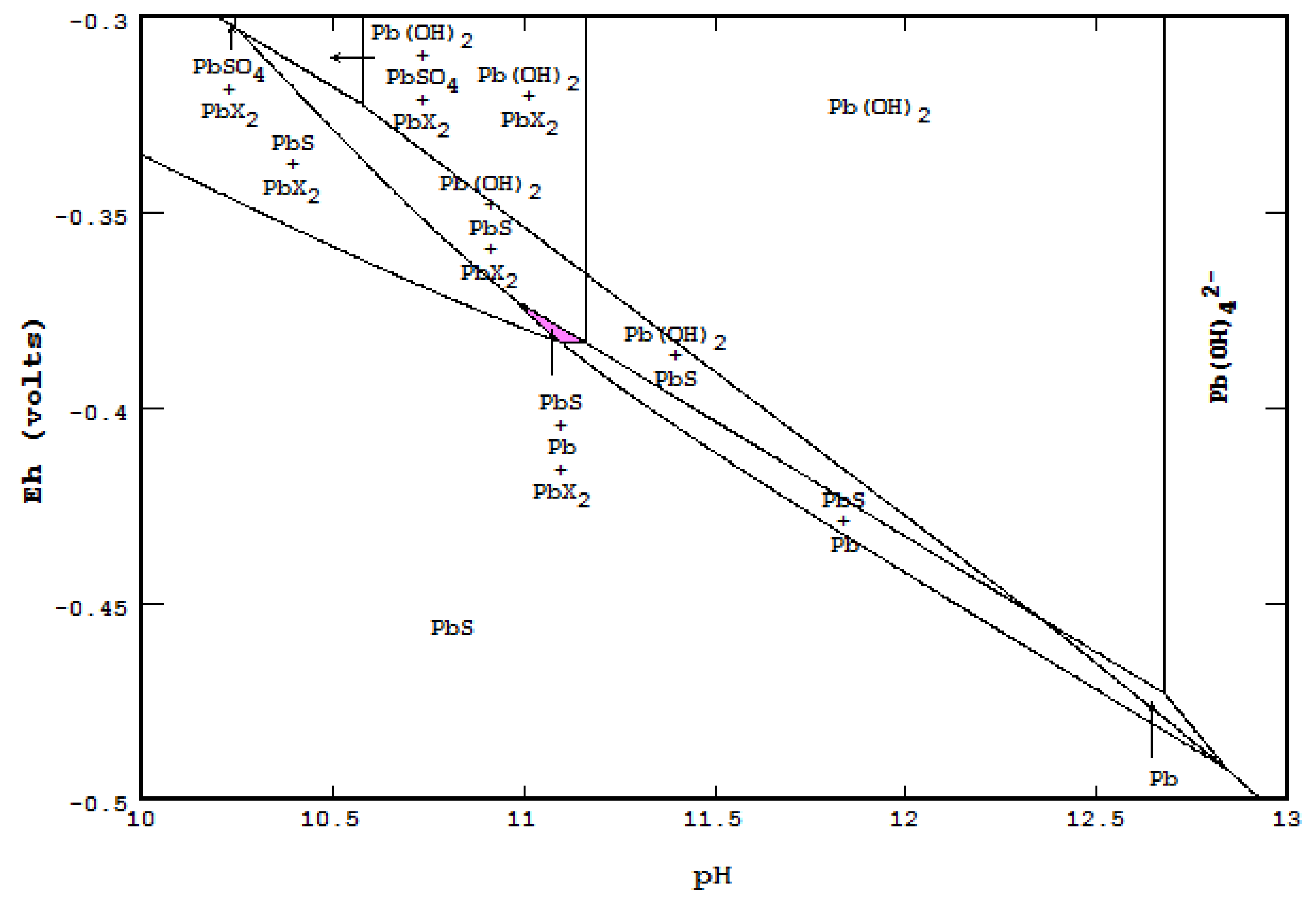
  23. Pritzker, M.D.; Yoon, R.H. Thermodynamic Calculations on Sulfide Flotation System: I. Galena-Ethyl Xanthate System in the Absence of Metastable Species. Int. J. Miner. Process. 1984, 12, 95–125. [Google Scholar] [CrossRef]
  24. Hiskey, J.B.; Wadsworth, M.E. Galvanic Conversion of Chalcopyrite. Metall. Trans. B 1975, 6, 183–190. [Google Scholar] [CrossRef]
  25. ParaView version 4.3.1 64-bit. Available online: http://www.paraview.org/download/ (accessed on 11 February 2015).
  26. VisIt 2015 Version 2.4.2. Available online: https://wci.llnl.gov/simulation/computer-codes/visit/ (accessed on 23 April 2012).
  27. MATLAB; Version R2013a; Mathworks Computer program: Natick, MA, USA, 2013.
  28. Grossmann, K.; Arnold, T.; Lkeda-Ohno, A.; Steudtner, R.; Geipel, G.; Bernhard, G. Fluorescence properties of a uranyl(V)-carbonate species [U(V)O2(CO3)3]5− at low temperature. Spectrochim. Acta A 2009, 72, 449–453. [Google Scholar] [CrossRef] [PubMed]
  29. VTK Format. The VTK User’s Guide, Version 4.2, Kitware. 2010. Available online: http://www.vtk.org/wp-content/uploads/2015/04/file-formats.pdf (accessed on 19 February 2015).

