CFD Modelling of Flow and Solids Distribution in Carbon-in-Leach Tanks

Abstract

The Carbon-in-Leach (CIL) circuit plays an important role in the economics of a gold refinery. The circuit uses multiphase stirred tanks in series, in which problems such as dead zones, short-circuiting, and presence of unsuspended solids are detrimental to its efficiency. Therefore, the hydrodynamics of such a system is critical for improving the performance. The hydrodynamics of stirred tanks can be resolved using computational fluid dynamics (CFD). While the flow generated by the impellers in the CIL tanks is complex and modelling it in the presence of high solid concentration is challenging, advances in CFD models, such as turbulence and particle-fluid interactions, have made modelling of such flows feasible. In the present study, the hydrodynamics of CIL tanks was investigated by modelling it using CFD. The models used in the simulations were validated using experimental data at high solid loading of 40 wt. % in a lab scale tank. The models were further used for examining the flow generated by pitched blade turbine and HA-715 Mixtec impellers in lab scale CIL tanks with 50 wt. % solids. The effect of design and operating parameters such as off-bottom clearance, impeller separation, impeller speed, scale-up, and multiple-impeller configuration on flow field and solid concentrations profiles was examined. For a given impeller speed, better solids suspension is observed with dual impeller and triple impeller configurations. The results presented in the paper are useful for understanding the hydrodynamics and influence of design and operating parameters on industrial CIL tanks.

1. Introduction

Carbon-in-Leach (CIL) circuit is a process that concentrates gold from 2.5 to 3.5 g/t in ore to 10,000 to 15,000 g/t on carbon. It is a process of continuous leaching of gold from ore to liquid and counter-current adsorption of gold from liquid to carbon particles in a series of tanks. The tanks used in the CIL circuit are continuously stirred tanks and contain high concentration of ores. Efficient operation of CIL tanks requires suspension of the ore particles in the leaching solution and hence, to provide maximum contact between ore and leaching solution. However, problems such as settled solids and presence of dead zones are detrimental to the efficiency, and could be identified and solved by understanding the flow field and solid distribution in the system. Furthermore, reducing the energy consumption to achieve a higher contact is always desired and can be achieved by proper design and optimization while investigating the hydrodynamics.

While, some information on the hydrodynamics such as residence time distribution (RTD) can be obtained from experiments using tracer studies; detailed quantitative measurement of the flow field inside the CIL tank is challenging. In such a scenario, computational fluid dynamics (CFD) can prove to be an inexpensive and viable solution. With the availability of improved models for turbulence, interphase drag force, particle-particle interaction models, etc. and advances in computational speeds, resolving the complex multiphase flows phenomenon is possible using CFD.

In the present work, models for simulating high solid loading stirred tanks are validated with experimental data. The flow field generated by a pitched blade turbine and a HA-715 impeller is compared. The effect of design parameters such as off-bottom clearance, impeller separation, impeller speed, scale-up, and multiple-impeller configuration is examined by modelling the flow and estimating the suspension quality for each case.

2. Literature Review

Carbon-in-leach tanks are high solid loading stirred tanks of large diameter (~10–15 m) with solid concentration of up to 50% by weight (~28% by volume). Such a high concentration renders opacity to the system which makes its hydrodynamic investigation challenging even at a small scale. With the advent of radioactive experimental techniques such as Computer Aided Radioactive Particle Tracking (CARPT), Positron Emission Particle Tracking (PEPT), etc., reliable quantitative data can be obtained [1,2,3]. The data can now be used to validate the computational models for the high solid loading regimes in turbulent flows and further advance the design and optimization of CIL tanks.

While simulating high solid concentration (20% by volume) stirred tanks, Altway et al. [4] found major discrepancy while validating the solid concentration profile using data from Yamazaki et al. [2]. Micale et al. [5] used Multiple Reference Frame (MRF) and Sliding Grid (SG) approach to study the clear liquid layer and the suspension height for dense solid-liquid systems. In their simulations, the power numbers were 2.98, 2.74, and 2.68 for N = 5, 6.33 and 8 RPS respectively (particle loading of 9.6% v/v), which were significantly smaller than the experimental values of 4.59, 4.37, and 4.23. They attributed the imperfection in the solid suspension prediction to second order effects (particle drag modifications due to liquid turbulence, presence of other particles, particle-particle direct interactions, etc.) that were neglected in the study. Ochieng and Lewis [6], Fradette, et al. [7], Ochieng and Onyango [8], Kasat, et al. [9], Fletcher and Brown [10], Tamburini, et al. [11,12,13], conducted simulations for volume fractions below 20%, and validated using non-local properties like cloud height, suspension quality, etc. In another similar study, Gohel, et al. [14] used qualitative and quantitative data for cloud height to validate the simulation of high concentration solids suspension in stirred tanks. In these studies, while the parameters, for example cloud height, were accurately predicted, the errors in the predictions of local hydrodynamics were not verified in the absence of data. In the direction of resolving the local hydrodynamics of the stirred tanks, Liu and Barigou [15] used local velocity field and solids concentration data for model validation and found that even though a good agreement in the axial concentration profile was observed, the local concentration predictions could still be very poor and could vary from experiments by several folds. The inaccuracy was attributed to inadequate models for particle sedimentation, lift-off, and particle-particle interaction in their CFD model. They suggested incorporating particle-particle interaction in the solids pressure term given by Gidaspow [16], but did not use it in their models due to convergence problems. The highest solid loading for which the simulation results in stirred tanks are reported is 20% (by volume), and the simulations are not able to predict the local concentration due to limitations of models [4,5].

In the CIL tanks, Dagadu, et al. [17] used a radioactive tracer to investigate the RTD in the CIL tanks and developed a model to predict it. While the results provided an overview of complexity of the system and suggested the presence of stagnant and active volumes, the details such as solid accumulation, dead-zones, uniformity, etc. are still unknown. To address these issues, Dagadu et al. [18,19] investigated the mixing in the CIL tanks by conducting CFD simulations and drawing inferences based on the flow field and eddy viscosity. In both of these instances, neither the relationship of the flow field or turbulent viscosity with the solid distribution is quantified, nor the solid distribution in the tanks are presented. While validation with experimental data is missing, the scope of both studies is limited to evaluating the ability of the models for predicting the qualitative flow behavior in such systems. Drawing conclusions for critical design and operating parameters requires comprehensive validation of models and controlled investigation of influence of these parameters on the flow field and solid distribution.

The current study focuses on the extensive validation of local solid concentration distribution in high solid loading stirred tanks. The shortcomings of previous investigations are addressed by using the appropriate constitutive models for turbulence, drag, particle-particle interactions, etc. The validated model is then used for investigation of critical parameters in the CIL tanks.

3. Model Description

3.1. Governing Equations

The hydrodynamic simulations are conducted using Eulerian-Eulerian multiphase model. In this model, each phase is treated as an interpenetrating continuum represented by a volume fraction at each point of the system. Reynolds averaged mass and momentum balance equations are solved for each phase. The governing equations are:

Continuity equation:

$$\frac{\partial }{\partial t}\left({\text{α}}_q{\text{ρ}}_q\right)+\nabla .\left({\text{α}}_q{\text{ρ}}_q{\overline{u}}_q\right)=0$$

(1)

Momentum equation:

$$\frac{\partial }{\partial t}\left({\text{α}}_q{\text{ρ}}_q{\overrightarrow{u}}_q\right)+\nabla .\left({\text{α}}_q{\text{ρ}}_q{\overrightarrow{u}}_q{\overrightarrow{u}}_q\right)=-{\text{α}}_q\nabla p+\nabla .{\stackrel{=}{\tau }}_q+{\text{α}}_q{\text{ρ}}_q\overrightarrow{g}+{\overrightarrow{F}}_{td,q,vm,lift}+{\overrightarrow{F}}_{12}$$

(2)

The rotation of impeller can be simulated using sliding grid approach (SG) or Multiple Reference Frame (MRF). While MRF provides reasonably accurate steady state solution, SG is found to be more accurate compared to MRF approach [20,21]. Therefore, SG will be used in the paper to simulate the impeller rotation.

Turbulence is not resolved in the RANS simulations and therefore, it needs to be modelled. Standard k-ε is the most commonly used model in the RANS simulations of stirred tanks [4,9,21,22,23,24,25]. However, it finds limitation in modelling anisotropic turbulence in the impeller discharge region and under-predicts turbulent kinetic energy in flow impingement region. RSM model predicts the Reynolds stresses by explicitly solving their governing equations. Hence, it resolves the anisotropic turbulence and results in improved predictions of turbulence in such regions [26]. Large eddy simulation (LES) also resolves the larger anisotropic turbulence scales while requiring simulation of complete domain with fine mesh, which is computationally expensive [27]. For the same scale, the computational requirement using LES can be 100 times higher than that for RSM simulation. Therefore, in this paper, RSM model is used for modelling turbulence.

The equations of Reynolds Stress Model (RSM) model for turbulence are given below.

$$\begin{array}{l}\frac{\partial }{\partial t}\langle u_i^{\text{'}}{u}_j^{\text{'}}\rangle +\nabla .\left({\overrightarrow{u}}_q{u}_i^{\text{'}}{u}_j^{\text{'}}\right)=\nabla .\left(C_s\frac{k\langle u_i^{\text{'}}{u}_j^{\text{'}}\rangle }{\epsilon }\nabla \langle u_i^{\text{'}}{u}_j^{\text{'}}\rangle \right)-C_1\frac{\text{ε}}{k}\left(\langle u_i^{\text{'}}{u}_j^{\text{'}}\rangle -\left(2/3\right){\text{δ}}_{ij}k\right)\\ -C_2\left(P_{ij}-\left(2/3\right){\text{δ}}_{ij}P-S_{ij}\right)-\left(2/3\right){\text{δ}}_{ij}\text{ε}\end{array}$$

(3)

$$\frac{\partial }{\partial t}\left({\text{ρ}}_q\text{ε}\right)+\nabla .\left({\text{ρ}}_q{\overrightarrow{u}}_q\text{ε}\right)=\nabla .\left(C_{\text{ε}}\frac{\text{ρ}k}{\text{ε}}\langle u_i^{\text{'}}{u}_i^{\text{'}}\rangle \nabla \text{ε}\right)+\frac{\text{ε}}{k}\left(C_{\text{1ε}}{G}_{k,q}-C_{\text{2ε}}{\text{ρ}}_m\text{ε}\right)$$

(4)

where C_s, C₁, C₂, C_1ε, C_1ε, and C_2ε are constants. And, $P_{ij}=-\langle u_i^{\text{'}}{u}_k^{\text{'}}\rangle \nabla .u_j-\langle u_j^{\text{'}}{u}_k^{\text{'}}\rangle \nabla .u_i$; $P=\frac{1}{2}{P}_{ii}$; ${\text{ρ}}_q={\displaystyle \sum _{i=1}^N{\text{α}}_i{\text{ρ}}_i}$; ${\overrightarrow{u}}_q=\frac{{\displaystyle \sum _{i=1}^N{\text{α}}_i{\text{ρ}}_i}{\overrightarrow{u}}_i}{{\displaystyle \sum _{i=1}^N{\text{α}}_i{\text{ρ}}_i}}$.

Eddy viscosity is computed from

$${\text{μ}}_{t,q}={\text{ρ}}_q{C}_{\text{μ}}\frac{k^2}{\text{ε}}$$

(5)

Evaluation of generation of turbulent kinetic energy is consistent with Boussinesq hypothesis and is computed as

$$G_{k,q}={\mu }_{t,q}\left(\nabla {\overrightarrow{u}}_q+\nabla {\overrightarrow{u}}_q^T\right):\nabla {\overrightarrow{u}}_q$$

(6)

The equation of conservation of granular temperature is given as:

$$\frac{3}{2}\left[\frac{\partial }{\partial t}\left({\text{α}}_s{\text{ρ}}_s{\Theta }_s\right)+\nabla .\left({\text{α}}_s{\text{ρ}}_s{\overrightarrow{u}}_s{\Theta }_s\right)\right]=-\left(p_s\stackrel{=}{I}+\nabla .{\stackrel{=}{\tau }}_s\right):\nabla {\overrightarrow{u}}_s+\nabla .\left(k_{{\Theta }_s}\nabla {\Theta }_s\right)-{\text{γ}}_{{\Theta }_s}+{\text{φ}}_{ls}$$

(7)

where $-\left(p_s\stackrel{=}{I}+\nabla .{\stackrel{=}{\tau }}_s\right):\nabla {\overrightarrow{u}}_q$ is the generation of energy by the solid stress tensor, $\nabla .\left(k_{{\Theta }_s}\nabla {\Theta }_s\right)$ is the diffusion of energy, ${\text{γ}}_{{\Theta }_s}$ is the collisional dissipation of energy and ${\text{φ}}_{ls}$ is the energy exchange between fluid and solid phase.

Table 1. Constitutive equations.

Description	Equations
Liquid-phase stress tensor	${\stackrel{=}{\tau }}_q={\text{α}}_q{\text{μ}}_q\left(\nabla {\overrightarrow{u}}_q+\nabla {\overrightarrow{u}}_q^T\right)+{\text{α}}_q\left({\text{λ}}_q-\frac{2}{3}{\text{μ}}_q\right)\nabla {\overrightarrow{u}}_q\stackrel{=}{I}$
Solid-phase stress tensor	${\stackrel{=}{\tau }}_s={\text{α}}_s{\text{μ}}_s\left(\nabla {\overrightarrow{u}}_s+\nabla {\overrightarrow{u}}_s^T\right)+{\text{α}}_s\left({\lambda }_s-\frac{2}{3}{\mu }_s\right)\nabla {\overrightarrow{u}}_s\stackrel{=}{I}$
Solid shear viscosity	${\text{μ}}_s={\text{μ}}_{s,col}+{\text{μ}}_{s,kin}+{\text{μ}}_{s,fr}$
Collisional viscosity	${\text{μ}}_{s,col}=\frac{4}{5}{\text{α}}_s{\text{ρ}}_s{d}_s{g}_{o,ss}\left(1+e_{ss}\right){\left(\frac{{\Theta }_s}{\text{π}}\right)}^{0.5}{\text{α}}_s$
Kinetic viscosity	${\text{μ}}_{s,kin}=\frac{{\text{α}}_s{\text{ρ}}_s{d}_s}{6\left(3-e_{ss}\right)}\left[1+\frac{2}{5}\left(1+e_{ss}\right)\left(3e_{ss}-1\right){\text{α}}_s{g}_{o,ss}\right]$
Frictional viscosity	${\text{μ}}_{s,fr}=\frac{p_s\text{sin}\phi }{2\sqrt{I_{2D}}}$
Solids pressure	$p_s={\text{α}}_s{\text{ρ}}_s{\Theta }_s+2{\text{ρ}}_s\left(1+e_{ss}\right){\text{α}}_s^2{g}_{o,ss}{\Theta }_s$
Radial distribution function	$g_{o,ss}={\left[1-{\left(\frac{{\text{α}}_s}{{\text{α}}_{s,\text{max}}}\right)}^{1/3}\right]}^{-1}$
Diffusion coefficient of granular temperature	$k_{\Theta s}=\frac{15{\text{α}}_s{\text{ρ}}_s{d}_s\sqrt{{\Theta }_s\text{π}}}{4\left(41-33\text{η}\right)}\left[\begin{array}{l}1+\frac{12}{5}{\text{η}}^2\left(4\text{η}-3\right){\text{α}}_s{g}_{o,ss}\\ +\frac{16}{15\text{π}}\left(41-33\text{η}\right){\text{ηα}}_s{g}_{o,ss}\end{array}\right]$
	where $\text{η}=0.5(1+e\text{ss})$
Collision dissipation energy	${\text{γ}}_{\Theta s}=\frac{12\left(1-e_{ss}^2\right)g_{o,ss}}{d_s\sqrt{\text{π}}}{\text{ρ}}_s{\text{α}}_s^2{\Theta }_s^{3/2}$

Table 1. Constitutive equations.

Description	Equations
Liquid-phase stress tensor	${\stackrel{=}{\tau }}_q={\text{α}}_q{\text{μ}}_q\left(\nabla {\overrightarrow{u}}_q+\nabla {\overrightarrow{u}}_q^T\right)+{\text{α}}_q\left({\text{λ}}_q-\frac{2}{3}{\text{μ}}_q\right)\nabla {\overrightarrow{u}}_q\stackrel{=}{I}$
Solid-phase stress tensor	${\stackrel{=}{\tau }}_s={\text{α}}_s{\text{μ}}_s\left(\nabla {\overrightarrow{u}}_s+\nabla {\overrightarrow{u}}_s^T\right)+{\text{α}}_s\left({\lambda }_s-\frac{2}{3}{\mu }_s\right)\nabla {\overrightarrow{u}}_s\stackrel{=}{I}$
Solid shear viscosity	${\text{μ}}_s={\text{μ}}_{s,col}+{\text{μ}}_{s,kin}+{\text{μ}}_{s,fr}$
Collisional viscosity	${\text{μ}}_{s,col}=\frac{4}{5}{\text{α}}_s{\text{ρ}}_s{d}_s{g}_{o,ss}\left(1+e_{ss}\right){\left(\frac{{\Theta }_s}{\text{π}}\right)}^{0.5}{\text{α}}_s$
Kinetic viscosity	${\text{μ}}_{s,kin}=\frac{{\text{α}}_s{\text{ρ}}_s{d}_s}{6\left(3-e_{ss}\right)}\left[1+\frac{2}{5}\left(1+e_{ss}\right)\left(3e_{ss}-1\right){\text{α}}_s{g}_{o,ss}\right]$
Frictional viscosity	${\text{μ}}_{s,fr}=\frac{p_s\text{sin}\phi }{2\sqrt{I_{2D}}}$
Solids pressure	$p_s={\text{α}}_s{\text{ρ}}_s{\Theta }_s+2{\text{ρ}}_s\left(1+e_{ss}\right){\text{α}}_s^2{g}_{o,ss}{\Theta }_s$
Radial distribution function	$g_{o,ss}={\left[1-{\left(\frac{{\text{α}}_s}{{\text{α}}_{s,\text{max}}}\right)}^{1/3}\right]}^{-1}$
Diffusion coefficient of granular temperature	$k_{\Theta s}=\frac{15{\text{α}}_s{\text{ρ}}_s{d}_s\sqrt{{\Theta }_s\text{π}}}{4\left(41-33\text{η}\right)}\left[\begin{array}{l}1+\frac{12}{5}{\text{η}}^2\left(4\text{η}-3\right){\text{α}}_s{g}_{o,ss}\\ +\frac{16}{15\text{π}}\left(41-33\text{η}\right){\text{ηα}}_s{g}_{o,ss}\end{array}\right]$
	where $\text{η}=0.5(1+e\text{ss})$
Collision dissipation energy	${\text{γ}}_{\Theta s}=\frac{12\left(1-e_{ss}^2\right)g_{o,ss}}{d_s\sqrt{\text{π}}}{\text{ρ}}_s{\text{α}}_s^2{\Theta }_s^{3/2}$

The stress-strain tensor in the momentum transfer equation is due to viscosity and Reynolds stresses that include the effect of turbulent fluctuations. Boussinesq’s eddy viscosity hypothesis is used for the closure of momentum transfer equation. The particle-particle interaction is modelled using kinetic theory of granular flow by assuming that its behavior similar to dense gas. Similar to the thermodynamic temperature of gases, the granular temperature is used to model the fluctuating velocity of particles [16]. The constitutive equations for momentum equation are given in Table 1.

3.2. Turbulent Dispersion Force

Turbulent fluctuations result in dispersion of phases from high volume fraction regions to low volume fraction regions. The turbulent dispersion force is significant when the size of turbulent eddies is larger than the particle size [9]. The effect of turbulence dispersion force on the hydrodynamics in CIL tanks, is incorporated using the Burns, et al. [28] model. The model equations for turbulence dispersion force are given below:

$${\overrightarrow{F}}_{td,q}=C_{TD}{k}_{pq}\frac{D_{t,q}}{{\text{σ}}_{pq}}\left(\frac{\nabla {\text{α}}_p}{{\text{α}}_p}-\frac{\nabla {\text{α}}_q}{{\text{α}}_q}\right)$$

(8)

3.3. Interphase Drag Force

Interphase drag is the resultant force experienced by the particle in the direction of relative motion due to a moving fluid. Since, the solids and liquid phases are treated as inter-penetrating, an inter-phase momentum exchange term is required. The interphase exchange force is calculated using the following expression given by Syamlal et al. [29]:

$$F_d=\frac{3{\text{α}}_l{\text{α}}_s{\text{ρ}}_l{C}_D\text{Re}}{4d_p{V}_{\text{r}}^3}\left({\overrightarrow{u}}_l-{\overrightarrow{u}}_s\right)$$

(9)

where, $V_{\text{r}}=0.5\left(A-0.06\text{Re}+\sqrt{{(0.06\text{Re})}^2+0.12\text{Re}(2A-B)+{(A)}^2}\right)$; $A={\text{α}}_g^{5.14}$; $B=0.8{\text{α}}_g^{2.28}$, for ${\text{α}}_g\le 0.85$; $B={\text{α}}_g^{3.65}$, for ${\text{α}}_g>0.85$.

The drag coefficient is calculated using an expression that has a form derived by Dalla Valle and Kenning [30]:

$$C_D={\left(0.63+\frac{4.8}{\sqrt{\text{Re}/V_{\text{r}}}}\right)}^2$$

(10)

4. Methodology and Boundary Conditions

4.1. Vessel Geometry

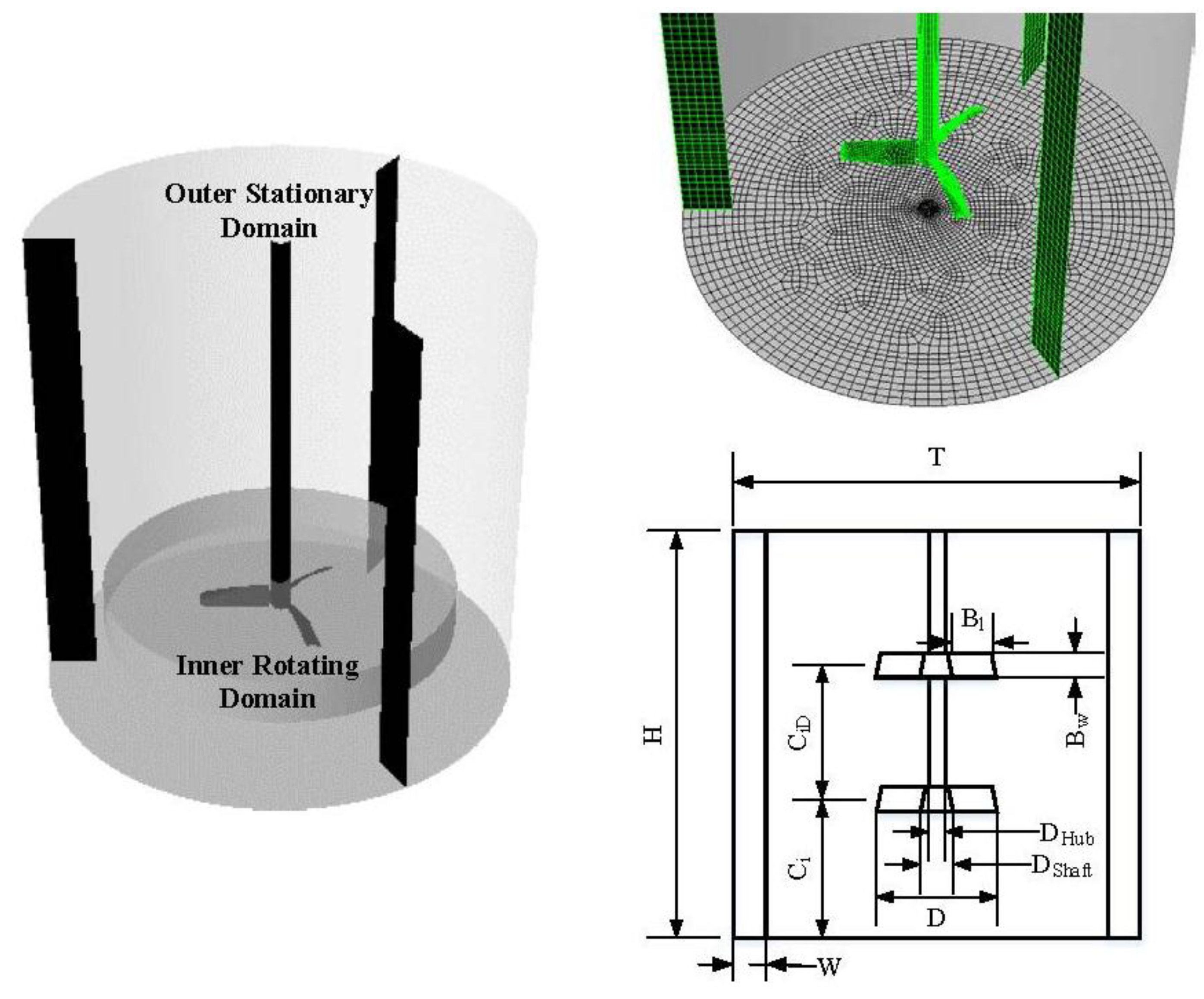
In this paper, a flat bottomed cylindrical tank was simulated (see Figure 1). The shaft of the impeller was concentric with the axis of the tank. A Mixtec HA-715 was used as impeller for CIL tanks, but for validation 45° six-bladed pitched blade turbine pumping downwards (PBTD) impeller was employed. For validation, vessel geometry dimensions, material properties, etc. were taken from paper of Guida et al. [3]. The dimensions of tank and impeller are given in Table 2. The fluid and particle properties used in the simulation are also tabulated in the same table. Conditions such as solid concentrations, impeller speed, and the Reynolds number in the tank are tabulated in Table 3. Simulations were carried out at just suspension speed for each case, which was determined by Guida et al. [3] following Zwietering [31] criterion. According to this criterion, no particle should remain stationary on the base of the vessel for longer than 1–2 s.

Figure 1. Computational domain, grid distribution, and schematic of the stirred tank.

Figure 1. Computational domain, grid distribution, and schematic of the stirred tank.

Table 2. Dimensions of domain and properties of materials used in this study.

Tank (m)		PBTD (m)		HA-715
T	0.288, 10	D	T/2	D	T/2, T/3
H	T	Bl	0.055	Dshaft	0.01152
W	T/10	Bw	0.041	-	-
Ci	T/2, T/3, T/4, T/6, T/8	Dshaft	0.01	-	-
		Dhub	0.034	-	-

Table 2. Dimensions of domain and properties of materials used in this study.

Tank (m)		PBTD (m)		HA-715
T	0.288, 10	D	T/2	D	T/2, T/3
H	T	Bl	0.055	Dshaft	0.01152
W	T/10	Bw	0.041	-	-
Ci	T/2, T/3, T/4, T/6, T/8	Dshaft	0.01	-	-
		Dhub	0.034	-	-

Table 3. Conditions in stirred tanks used for simulations.

Name of Case	X (wt. %)	N = Njs (RPM)	ρl (kg/m3)	µl (Pa·s)	ρp (kg/m3)	dp (mm)
PBTD-Validation	40	589.8	1150	0.001	2585	3
CIL tanks (Lab Scale)	50	200–700	1000	0.001	2550	0.075
CIL tanks (Full Scale)	50	22.15	1000	0.001	2550	0.075

Table 3. Conditions in stirred tanks used for simulations.

Name of Case	X (wt. %)	N = Njs (RPM)	ρl (kg/m3)	µl (Pa·s)	ρp (kg/m3)	dp (mm)
PBTD-Validation	40	589.8	1150	0.001	2585	3
CIL tanks (Lab Scale)	50	200–700	1000	0.001	2550	0.075
CIL tanks (Full Scale)	50	22.15	1000	0.001	2550	0.075

4.2. Numerical Simulations

The stirred tank for validation consists of six PBT blades and four baffles and that of CIL tanks consists of three HA-715 blades and three baffles. In all the cases studied in the paper, simulation of the full tank is conducted. For the case of PBTD, the moving zone with dimensions r = 0.06 m and 0.036 < z < 0.137 is created (where z is the axial distance from the bottom). For the case of HA-715, the moving zone of height T/10 and r = 3T/4 is created, with top and bottom surfaces equidistant from the center of impeller. The impeller rod outside this zone is considered as a moving wall. Impellers used in all the cases simulated in the study are operated in the down-pumping mode. The top of the tank is open, so it is defined as a wall of zero shear. The solids in the tank are assumed to be settled in the beginning of simulations. Therefore, a solid volume fraction of 0.6 is patched in the stirred tank up to a height such that the volume averaged solid concentration is the same as the uniformly distributed solids specified in Table 3. For modelling the turbulence, a RSM turbulence model is used. The standard model parameters are C_µ: 0.09, C_s: 0.22, C₁: 1.8, C₂: 0.6, C_1ε: 1.44, C_2ε: 1.92, σ_k: 1.0 and σ_ε: 1.3. In the present work, SIMPLE scheme is used for Pressure-Velocity coupling along with the standard pressure interpolation scheme. To avoid any numerical diffusion and unphysical oscillations, a third order Quadratic Upstream Interpolation for Convective Kinetics (QUICK) discretization scheme is used for momentum, volume fraction, turbulent kinetic energy, and turbulent dissipation rates. The convergence of the simulation is verified by monitoring residual values as well as additional parameters namely turbulence dissipation over the volume, turbulence dissipation at the surface right below impeller and torque on the shaft. Once the residuals and additional parameters are constant, a simulation is deemed to be converged. For all the cases presented in the paper, a time-step of 0.001 s is less than the time which the impeller needs to sweep by a single computational cell (one cell time step ~0.003 s). One cell time step is considered appropriate for the CFD simulations in stirred tanks [12]. But using a time-step of 0.001 s resulted in divergence in the initial time-steps. Therefore, the time-step size initially used in the simulations is 0.0001s, which is gradually increased to 0.001 s. For the full scale geometry, the one cell time step increased due to the reduction in the impeller speed. Therefore, the maximum time-step used for full-scale simulation is 0.01 s (one cell time step ~0.025 s). The results of lab scale simulations approached transient steady values after 12 s. Therefore, the data used for results and discussion is time averaged for the last 3 s. For full scale simulations, the time taken for reaching the transient steady value is 900 s, and the data is time-averaged for 300 s. The numerical solution of the system is obtained by using the commercial CFD solver ANSYS FLUENT 15.0 using 48 cores of Magnus with Cray XC40, Intel Xeon E5-2690V3 “Haswell” processors running at 2.6 GHz system at Pawsey supercomputing center. Each time step takes an average of 20 s of the wall clock time which reduces after approaching convergence when residuals reach at 10⁻⁵.

The finite volume method solves the partial differential equations in a spatially discretized domain. The discretization should be fine enough to resolve the physics while not incurring excess computational power. For the purpose, a grid independency test is conducted initially on the single phase flow and is presented. The models used in the paper are validated with the experimental results at 40 wt. % solid loading stirred tank published by Guida et al. [3]. The validated model is used for analyzing the flow field generated by HA-715 impeller and assessing its efficacy compared to the PBTD. The influence of different impeller speeds, impeller off-bottom clearance and impeller diameter on the solid suspension, homogeneity and power consumption are examined. The appropriate stirred tank design parameters are used for scale-up and simulations and are conducted to gain an insight on the flow developed. Flow generated by single and multiple impeller systems in the full-scale CIL tanks is also investigated.

5. Results and Discussion

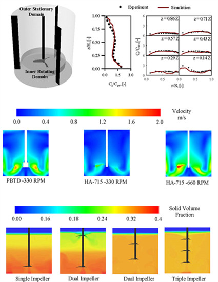
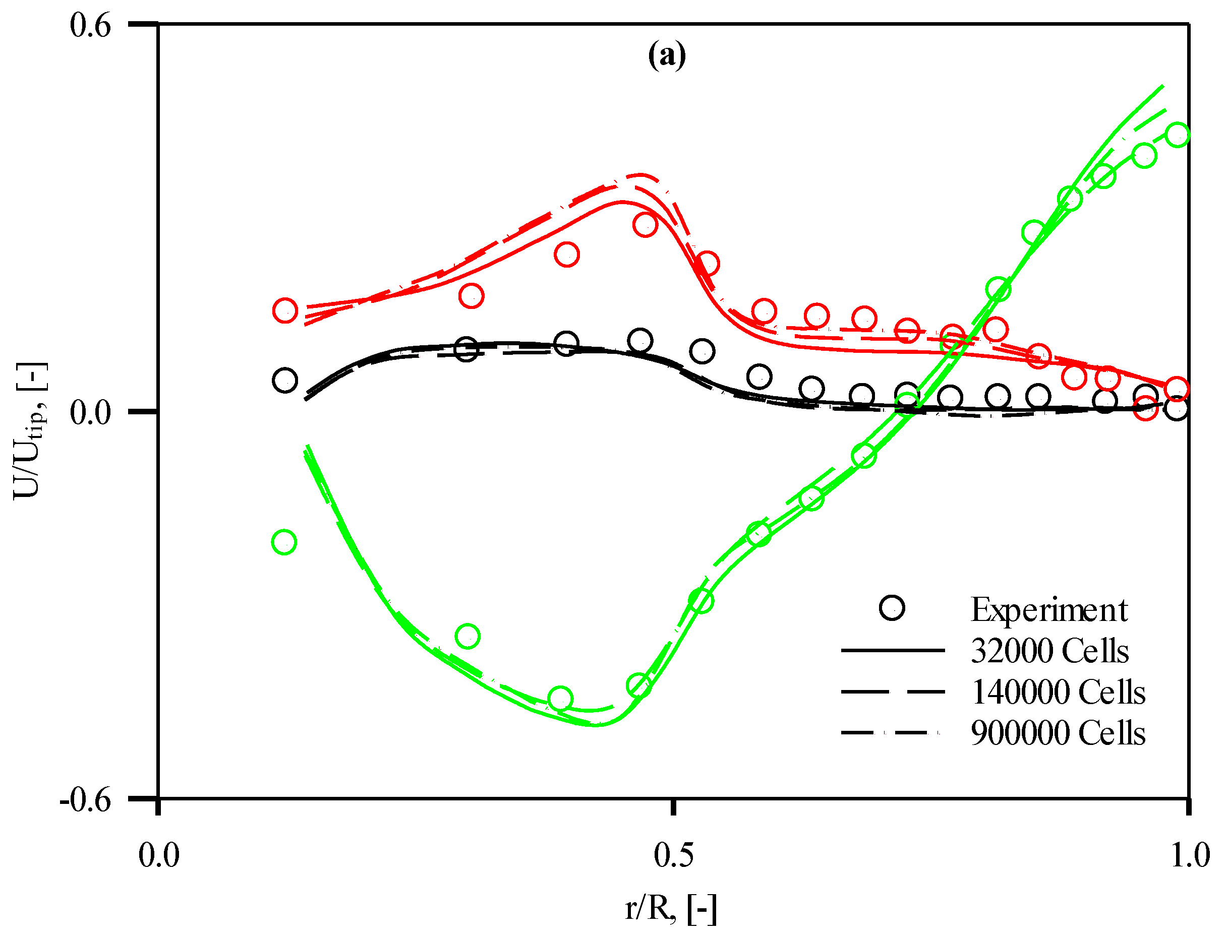
5.1. Grid Independency and Validation

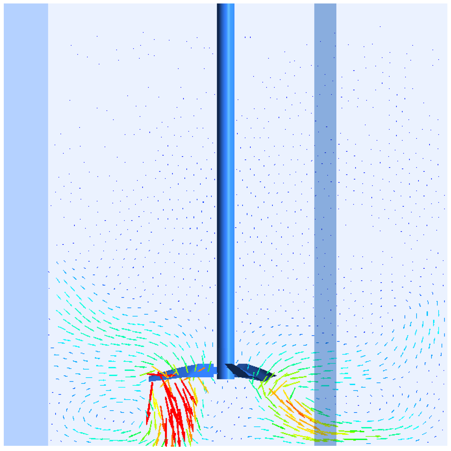
For testing the grid-independency, the experimental values for axial, tangential, and radial velocities at impeller discharge plane for single phase flow were compared with the simulation results using computational grids with 32,000 (coarse), 140,000 (medium) and 900,000 (fine) cells (see Figure 2). The results using mesh with 32,000 cells are accurate at z = 0.2 H plane. The predictions improve slightly while using 140,000 cells, and beyond that the improvement is marginal. Furthermore, the power for the stirred tanks is calculated by integrating the turbulence dissipation rate over the volume. For the coarse, medium, and fine meshes, the values of power number are 1.34, 1.53, and 1.57, respectively, which re-emphasizes that a mesh of 140,000 cells is suitable for simulation and further refinement will only lead to marginal improvement at significant computational cost. Therefore, the mesh with 140,000 cells is used for the rest of the simulations in the study. For the full scale geometry, the computational grid of 140,000, 900,000, and 3,000,000 cells are investigated based on the same parameters. The values of power number obtained for the three cases are 1.27, 1.49, and 1.55, respectively. Mixing time is another parameter that is sensitive to the number of computational cells in the domain. For the full scale tank, the mixing time for the three cases are 75 s, 113 s, and 111 s respectively to achieve 99% homogeneity. It is evident from the analysis that the results of 900,000 cells and 3,000,000 cells are similar. Therefore, the grid of 900,000 cells was selected for the simulation of full scale CIL tanks.

The models used in the study are validated by comparing the flow field generated by PBTD and the concentration profiles obtained at 40 wt. % solid loading. The axial, tangential, and radial velocity plots describe the flow generated by the PBTD. The PBTD pumps the fluid downwards leading to highly negative axial velocities at the impeller plane. The jet leaving the impeller flows down to the bottom of the stirred tank, is then redirected towards the periphery and circulates back to the top along the walls. Due to such motion, a flow loop is formed near the impeller. It results in decreasing axial velocity when moving radially outwards in impeller plane that eventually increases due to the upwards flow near the walls. A 45° inclination of the impeller blade imparts momentum in the tangential direction resulting in moderate values of tangential velocity. Due to the downward flow developed by a PBTD, the magnitude of the radial component of velocity is the lowest. The maximum values of radial, tangential, and axial velocity in the impeller plane are 0.1 U_tip, 0.28 U_tip, and 0.45 U_tip respectively. Both radial and tangential components gain value with the increase in radius as the velocity increases radially along the impeller blades. The maximum value is attained by both of these components close to the impeller tip after which a sudden decline is observed due to no momentum source in the absence of impeller. These characteristics are well represented in the velocity profiles shown in Figure 2.

Figure 2. Comparison of dimensionless axial (green), radial (black) and tangential (red) velocity at z = 0.2H plane for computational grid with different resolution.

Figure 2. Comparison of dimensionless axial (green), radial (black) and tangential (red) velocity at z = 0.2H plane for computational grid with different resolution.

The average axial concentration profile is compared with the experimental data of Guida et al. [3] in Figure 3a. In some cases, the average axial concentration does not provide the information for local variation of concentration. Therefore, radial concentration profiles at different heights are also compared with the experiments. As is evident from Figure 3, the results obtained are in agreement with the experimental data. As the impeller speed used is the speed of just suspension, the solid concentration near the bottom of the tank is only double the average concentration. The jet from the PBTD moves downwards and strikes the bottom around the r/R = 0.5. Therefore, the concentration at this location is low. However, the solid is accumulated at the bottom center and the bottom corner of the tanks due to low velocity fields in both of these regions. Near 0.29 Z, the low concentration in the loop of the eye formed by the jet circular loop is also well predicted by the simulations. With increasing height, the axial velocity near the wall and impeller diminish and therefore, the concentration profile also becomes inverted with low concentration near the periphery and impeller rod. This shape of concentration profile is maintained till the top of the stirred tank with the magnitude of concentration decreasing with height.

The validity of the CFD simulations is further tested by comparing the results of cloud height in stirred tanks. For quantifying the cloud height, Hicks et al. [32] conducted experiments and reported the values at various suspension speeds, D/T, power, torque, and suspension ratios. Bittorf and Kresta [33] developed a model for predicting the cloud height based on the analysis of liquid jet velocity and just suspension speed. Due to inherent complexity due to several variables such as solid concentration, suspension speed, particle diameter, D/T ratio, C/T ratio, experimental errors, etc., error in the predictions lie in the range of ±16%. Therefore, the simulations are conducted using 10.6% solid concentration (by weight) at N_js with D/T of 0.5 and C/T of 0.25. These results were compared with the experimental results of Hicks et al. [32]. The cloud height obtained from CFD simulations is 0.93 compared to the experimental value of 0.94. For the solid concentration of 20% and 40%, the cloud height calculated from CFD simulation is 0.935 and 0.942 respectively. This aligns with the observation by Hicks et al. [32] that the cloud height remains nearly constant between solid concentration of 10% and 40%. It is evident that the models used in the simulations are able to predict the local hydrodynamics for high solid loading stirred tank systems accurately and can be used for investigating hydrodynamics in CIL tanks.

Figure 3. (a) Averaged axial concentration profiles and (b) radial concentration profiles plotted at different heights in stirred tanks with 40 wt. % solid loading using PBTD.

Figure 3. (a) Averaged axial concentration profiles and (b) radial concentration profiles plotted at different heights in stirred tanks with 40 wt. % solid loading using PBTD.

5.2. Flow Field

The simulations of lab scale stirred tank with PBTD and HA-715 were conducted to compare the hydrodynamics in both the cases. Only for these set of simulations, four baffles were employed for the HA-715 case, which is equal to that of PBTD cases. The flow field generated by both axial impellers viz. PBTD and HA-715 are shown in Figure 4. The asymmetry seen in the case of HA-715 impellers is due to the use of three impeller blades which cannot simultaneously appear in the mid-baffle plane. Both of these impellers generate strong axial flow with similar flow field profile. Similar to the flow generated by PBDT, the jet originates from the impeller blades for HA-715 impeller and strikes the bottom of the tank. Such a motion is effective for the suspension of ore particles at the bottom of the tank. After hitting the bottom, the fluid changes direction and moves upwards along the wall of the stirred tank. This results in higher axial velocities near the bottom-wall region of the stirred tanks, where both radial and tangential velocities diminish. The value of axial velocity near the wall gradually diminishes with the ascent due to the counter effect of gravity. The height to which axial velocity remains significant is proportional to the magnitude of velocity at the bottom, which exerts force against gravity. Such a behavior is also evident from Figure 4. It can be observed from contours that for the same impeller rotation speed, the flow generated by PBTD is dominant compared to that generated by HA-715. However, the flow generated at a particular impeller rotation speed is not the sole criterion for determining the efficacy of impellers. Rather than the impeller speed, the power consumed is a more reasonable criterion, where the desired flow needs to be generated by supplying a specific amount of power. While the power consumed for the PBTD case is 20.79 W, its value for the HA-715 case at 300 RPM is only 3.25 W. Therefore, the power used in HA-715 was increased to 12.89 W by doubling the impeller speed. This change resulted in a flow field that is far more effective than that generated by the PBTD, while using 60% of the power. The efficiency of mixing for both the cases is quantified by determining the mixing time using an 8% solute patched at the top of stirred tank. The value of mixing time for PBTD is 4.2 s, while the same for HA-715 at 660 RPM is 2.9 s. Therefore, for the given power consumption, HA-715 shows better mixing characteristics than PBTD.

Figure 4. Flow field contours in a stirred tank generated by PBTD and HA-715.

Figure 4. Flow field contours in a stirred tank generated by PBTD and HA-715.

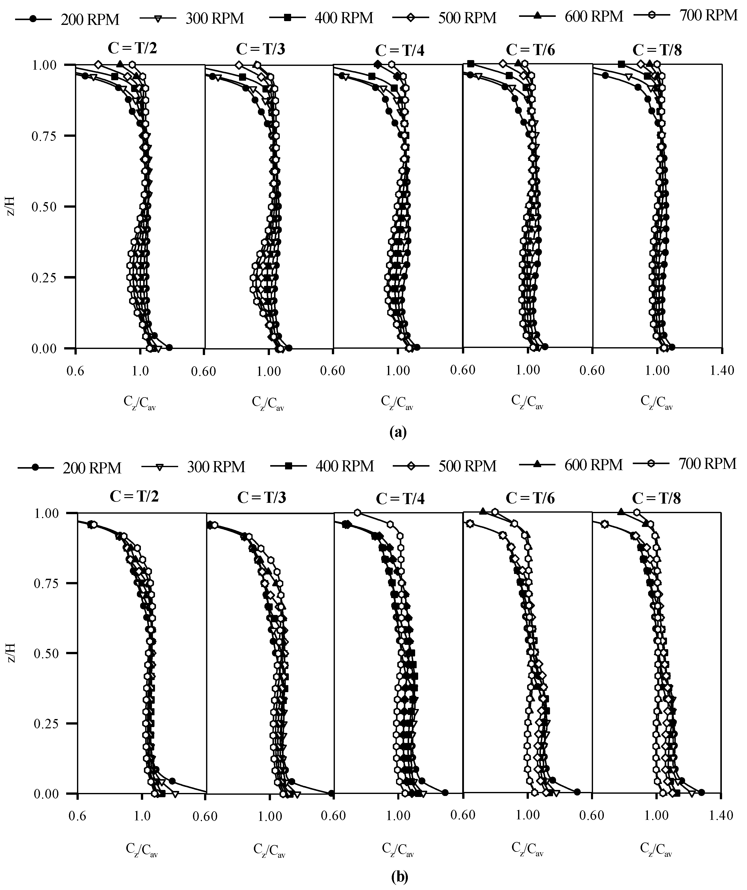
5.3. Concentration Profiles

The CIL stirred tanks at 50 wt. % solid loading are simulated at lab scale. The influence of impeller speed, diameter, and off-bottom clearance is analyzed by plotting the concentration profiles for each of the cases in Figure 5. The variation of off-bottom clearance and impeller speed presented in this paper is between 0.125 T and 0.5 T, and 200 and 700, respectively. These variations are studied for impeller diameters of 0.5 T and 0.33 T.

At low off-bottom clearance for the impeller diameter of 0.5 T, the concentration profile remains uniform in the bottom half of the tank. It suggests the lower off-bottom clearance contributes to suspension of the settled solids. Therefore, the rise in the solid concentration near the bottom is not visible for C = T/8 case. As the clearance is gradually increased, the velocity of jet hitting the bottom also decreases, and hence the possibility of the presence of settled solids increases. The presence of settled solid at the bottom is dependent on the velocity of jet when it hits the bottom. Also this velocity is governed by the distance between the impeller and the bottom, and the impeller rotation speed. For high off-bottom clearance and low impeller rotation speeds, the jet velocity hitting the bottom is low, and hence a higher solid concentration can be observed near the bottom of the tank. With the increase in the off-bottom clearance, solid concentration assumes a vertically flipped S-shaped profile. This profile is an indication of significant variation in the solid concentration with height. Such a profile means, the concentration of solid is high at the bottom, it lowers around the region of impeller, then gradually increases above the impeller, and then finally diminishes near the top of the stirred tanks. Comparatively lower concentration in the region near the impeller is because the jet carrying solids circulates after hitting the bottom, and forms an eye with very low velocity at the center, resulting in lower solid accumulation in this region. In all the cases in which the lower concentration is observed, a circular loop formed by the jet is present. Therefore the presence of circular loop and the magnitude of the jet velocity determines the formation of a low concentration zone near the impeller. This circular loop is not formed in two cases: first, at low impeller speeds and high off-bottom clearance as the velocity diminishes before the jet reaches the bottom of the tank; and second, at low off-bottom clearance, where the jet hits the bottom but cannot get enough distance to form a loop. In both of these cases, a flat profile near the impeller is observed.

Figure 5. Axial concentration profiles at different stirrer speeds and off-bottom clearance for impeller to tank diameter ratio of (a) 0.5 and (b) 0.33.

Figure 5. Axial concentration profiles at different stirrer speeds and off-bottom clearance for impeller to tank diameter ratio of (a) 0.5 and (b) 0.33.

When the impeller diameter is decreased to 0.33 T, the flipped S-shaped concentration profile is not dominant. On the contrary, the concentration is high near the bottom, which decreases to average concentration while reaching the height of the impeller, and then gradually decreases when reaching near the top. Clearly, the conditions for strong circular loop formed in the 0.5 T case is not met in the 0.33 T case. With the decrease in the impeller diameter and similar rotation velocity, the impeller tip speed is reduced and therefore, the velocity magnitude of the jet is not sufficient to form a circular loop of solids. Therefore, the profiles for all the cases are almost identical, with strong influence of impeller speed. At low impeller speeds, a high accumulation of solids at the bottom and low concentration at the top is observed. At high impeller speeds, the concentration values showed less variation with height. However, the influence of off-bottom clearance on the accumulation of solid near the bottom remained the same as in the case of 0.5 T. A low off-bottom clearance is found beneficial to suspend the settled solids.

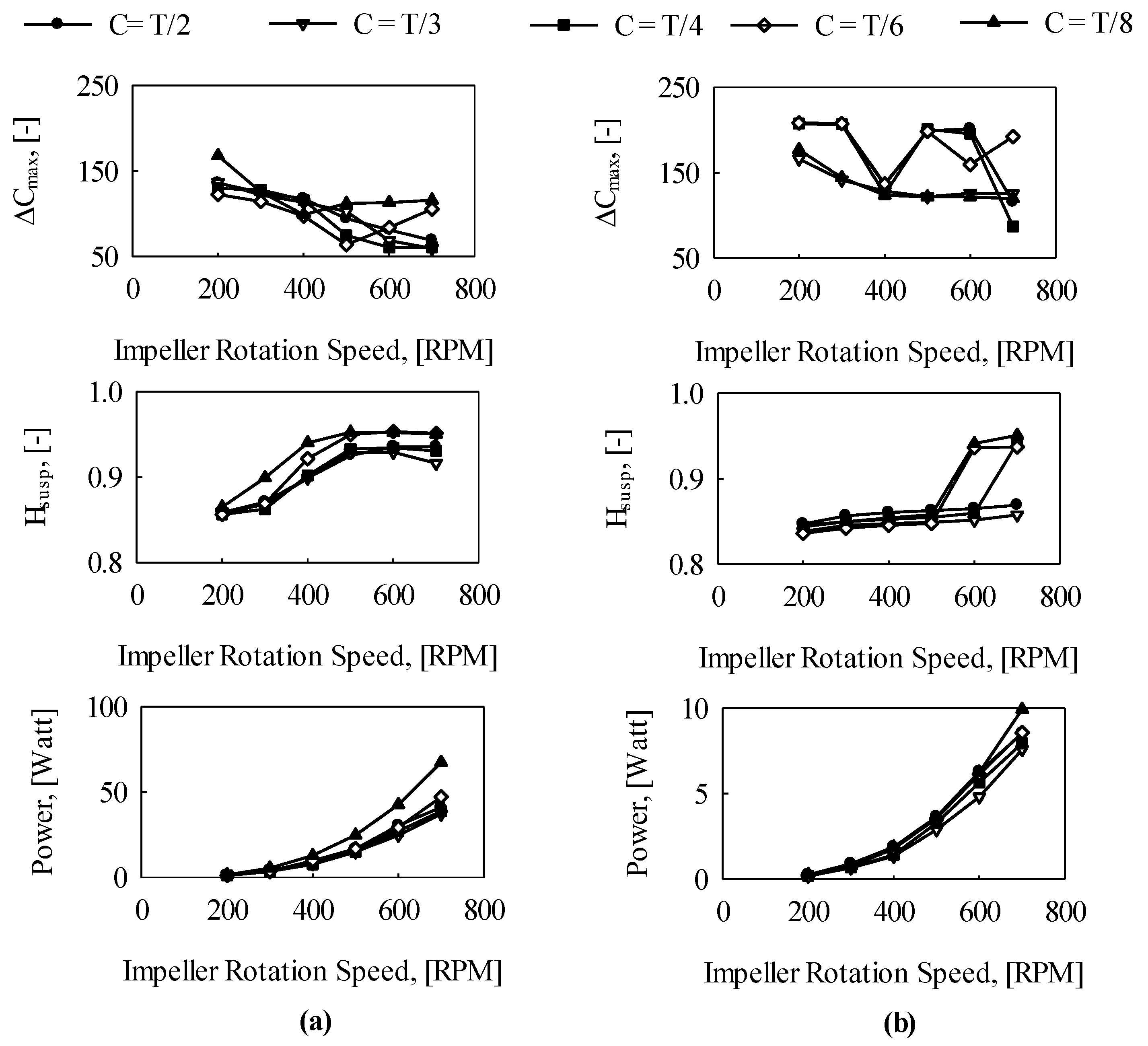
5.4. Suspension Quality and Power Consumption

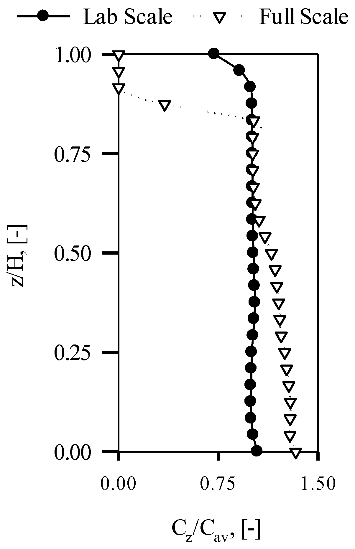
The suspension quality and power consumption are the two important parameters for determining the efficiency of a stirred tank. A high homogeneity (high suspension quality) achieved at a low power consumption is the objective of design and optimization. Suspension quality in a stirred tank can be defined in two different ways: first, by defining the variation between the minimum and maximum concentration [34] and second, by determining the homogeneity by variation in local concentration compared to the average concentration [35]. Mathematical representation of both these methods is given in equations below:

$$\Delta C_{\text{max}}=\frac{C_{\text{max}}-C_{\text{min}}}{C_{\text{average}}}\times 100$$

(11)

$$H_{\text{susp}}=1-\sqrt{\frac{1}{n}{{\displaystyle \sum _{i=1}^n\left(\frac{C_i}{C_{\text{average}}}-1\right)}}^2}$$

(12)

The results obtained from both of these equations are plotted in Figure 6. While the results from the H_susp equation suggest that the homogeneity increases with the increase in impeller speed and reaches a plateau value, the results of the ΔC_max equation appear quite erratic. Such an observation is a result of error in the C_min or C_max values due to local errors during computation. Therefore, a conclusion cannot be drawn from these plots with confidence. H_susp provides insight with respect to the homogeneity prevailing in the stirred tanks.

For the case of D_i/T = 0.5, the homogeneity is low at low impeller speeds, which improves with increasing impeller speed and reaches a plateau. However, for an impeller off-bottom clearance of T/3, the homogeneity decreases at very high velocity because of the generation of a dominant flipped S-shaped concentration profile (see Figure 5a). For a clearance higher than T/3 or lower than T/3, the flipped S-shaped profile is not dominant and therefore, the decrease in homogeneity at very high impeller speed is also not observed. The highest deviation in the homogeneity occurs due to the suspended solids at the bottom. Decreasing the off-bottom clearance allows the high velocity jet to force the solids to suspend. Therefore, at off-bottom clearance of T/8, the homogeneity improves at lower impeller speed compared to other cases.

Figure 6. Suspension quality and power consumption plotted at different stirrer speeds and off-bottom clearance for impeller to tank diameter ratio of (a) 0.5 and (b) 0.33.

Figure 6. Suspension quality and power consumption plotted at different stirrer speeds and off-bottom clearance for impeller to tank diameter ratio of (a) 0.5 and (b) 0.33.

The results of cases D_i/T = 0.33 are far different from those of D_i/T = 0.5. In these cases, the improvement in the homogeneity is not significant with the increase in the impeller rotation speed. Exceptions are the case of off-bottom clearance of T/4, T/6, and T/8, where the homogeneity crosses 0.9 beyond the impeller rotation speed of 600, 500, and 500 RPM respectively. This suggests that the higher off-bottom clearance and low impeller speeds result in dead zones in the stirred tank, hence reducing the homogeneity. When the velocities in the lower part of the tank are sufficiently high, the solids suspend and a higher value of homogeneity is achieved.

For a particular impeller speed, the power consumption in a stirred tank system is proportional to $D_i^5$. Therefore, the power consumption for an impeller diameter of D_i/T = 0.5 is higher than that of D_i/T = 0.33 at a given RPM (see Figure 6). For an impeller rotation speed of 700 RPM, the power consumption for cases of D_i/T = 0.33 is less than 9 W. The impellers with D_i/T = 0.5 can operate only up to 400 RPM using this power, and beyond 400 RPM, these impellers will require additional power. However, at the same time, homogeneity higher than a value of 0.9 can only be achieved for an impeller rotation speed above 400 RPM using this impeller diameter, while the same can be achieved using an impeller diameter of D_i/T = 0.33 and clearance of T/6 or T/8 using 70% of the power requirement at 600 RPM. Therefore, D_i/T = 0.33 is more efficient than D_i/T = 0.5 for obtaining high suspension quality for a given power consumption. The power consumption also varies with the off-bottom clearance [36]. The closer the impeller is to the bottom of the tank, the higher the turbulence and power dissipation. Although only minor, the power consumption of T/8 off-bottom clearance is more than that of T/6. Therefore out of all the cases discussed, the impeller diameter of D_i/T = 0.33 with clearance of T/6 and impeller rotation speed of 600 RPM is appropriate for efficiently suspending high concentration of solids in a stirred tank using an HA-715 impeller.

5.5. Scale-Up

Different scale-up criteria are available based on attaining homogeneity or complete suspension condition in the stirred tanks [37,38,39,40]. Buurman et al. [37] suggested a scaling up rule of $N_{\text{js}}\propto D^{-0.666}$ for the complete suspension in stirred tanks assuming the turbulence to be isentropic. Barresi and Baldi [40] suggested that $N_{\text{js}}\propto D^{-0.666}$ is strictly valid in a homogeneous isotropic turbulent field and devised a new rule of $N_{\text{js}}\propto D^{-0.666}$ by applying the turbulence theory to the solids distribution. Magelli et al. [38] investigated the solids distribution in high aspect ratio stirred tanks under batch and semibatch conditions and found that a constant ND^0.93 was more appropriate. Montante et al. [39] analyzed the scale-up criteria for stirred tanks based on the dependency of minimum impeller speed as a function of impeller diameter and the dependency of settling velocity on the λ/dP, and backed the scale-up criterion of a constant ND^0.93. Montante et al. [41] further investigated the role of turbulence on the particle settling and suspension in scaled-up vessels, and arrived at the conclusion that intermediate turbulent fluctuation maintains the vertical solid concentration. Therefore, a value intermediate of constant tip speed $N_{\text{js}}\propto D^{-1}$) and constant power per unit volume ($N_{\text{js}}\propto D^{-0.666}$), i.e., $N\propto D^{-0.93}$ is appropriate for scaling-up. Based on this criterion, an impeller velocity of 22.15 RPM used for a stirred tank with T = 10 m.

The axial concentration profiles in laboratory scale and full scale stirred tanks are shown in Figure 7. The homogeneity in solid concentration observed in the laboratory scale stirred tank at 600 RPM is not extrapolated to the full scale stirred tank at 22.15 RPM. The presence of low concentration on the top can be explained by the very low velocity field present in the top part of the full scale tank (see Figure 8). The velocity imparted by the impeller is observed to be localized in the lower part of the stirred tank and has apparently no influence on the top. Therefore, the velocity vectors between the middle and top of the impeller are nearly invisible showing low velocity zones. The average value of turbulent kinetic energy in the lower half of the tank is 0.033 m²/s², which reduces to 0.0008 m²/s² in the lower half of the tank. Without sufficient kinetic energy in the flow field in this zone, the settling of solids is evident. As a result, the solid concentration drops sharply to zero after 8.5 m in the full scale tank. Due to the same low velocity field in the middle to top zone of the stirred tank, the remaining solid stays suspended in the bottom half of the stirred tank.

From the above discussion it is clear that the power provided in the lower half of the stirred tank is sufficient to suspend the solids. However, due to the absence of a power source in the upper half, maintaining the homogeneity in the stirred tank is not possible. Therefore, a multiple impeller system is desired to achieve homogeneity.

Figure 7. Axial concentration profiles for lab scale (T = 0.288 m) and full scale (T = 10 m) stirred tanks with C = T/6 and D_i = T/3.

Figure 7. Axial concentration profiles for lab scale (T = 0.288 m) and full scale (T = 10 m) stirred tanks with C = T/6 and D_i = T/3.

Figure 8. Velocity vectors on baffle-impeller blade plane in a full scale stirred tank.

Figure 8. Velocity vectors on baffle-impeller blade plane in a full scale stirred tank.

5.6. Multiple-Impeller Systems

As the homogeneity was not achieved with the single impeller and additional power for solid suspension near the top is required, more impellers are required to be installed in the full scale CIL tanks. Therefore, three configurations in multi-impeller CIL systems were investigated, the details of which are given in Table 4.

Table 4. Details of impeller configuration in multi-impeller CIL tanks.

Variable	Twin-CT6	Twin-CT3	Triple-CT4
Off-bottom clearance, Ci	T/6	T/3	T/4
Distance between impellers, CiD	2T/3	T/3	T/4

Table 4. Details of impeller configuration in multi-impeller CIL tanks.

Variable	Twin-CT6	Twin-CT3	Triple-CT4
Off-bottom clearance, Ci	T/6	T/3	T/4
Distance between impellers, CiD	2T/3	T/3	T/4

The solid concentration contours on the baffle-impeller plane in the full-scale CIL tanks for single impeller and multi-impeller cases are given in Figure 9. The inhomogeneity in the single and Twin-CT6 cases are evident from the contour plot. A continuous gradient is observed from bottom-to-top in these two cases. This gradient can be categorized into three zones of very low, medium, and high solid concentration. The use of a second impeller in the Twin-CTby6 case forms a jet that draws the low concentration liquid from the top and circulates the high concentration fluid along the periphery of the tank. Such a flow is favorable for increasing the suspension quality near the top of the CIL tanks, as a result of which the extent of the low concentration zone is reduced. The zone of high solid concentration is the largest for the single impeller system (extends to z = 0.6 T), which is reduced by using a second impeller which disperses the high solid concentration present near the middle of the CIL tanks (extends to z = 0.5 T). However, the limited range of the jet formed by this impeller does not significantly affect the high concentration zone which still extends to half of the tank. Nonetheless, the use of a second impeller is partially effective in improving the homogeneity.

Figure 9. Concentration profiles in baffle-impeller plane for (a) Single impeller; (b) Twin-CT6; (c) Twin-CT3 and (d) Triple-CT4.

Figure 9. Concentration profiles in baffle-impeller plane for (a) Single impeller; (b) Twin-CT6; (c) Twin-CT3 and (d) Triple-CT4.

While, the presence of impeller near the gradient at the top was found beneficial, a similar approach near the interface between medium and low concentration zones can be applied. Therefore, Twin-CT3 and Triple-CT4 cases were investigated specifically targeting at the interface of the gradients between the zones. The strategy appears to be beneficial as the interface between the medium and high concentration zone disappears and an intermediate concentration is observed to be prevalent in the majority of tank. The average concentration values of intermediate concentration zones for Twin-CT3 and Triple-CT4 cases are 0.32 and 0.31, respectively. The increased distance from the top in Twin-CT3 case results in the weakening of drawing forces at the interface of low and medium concentration zones. Therefore, compared to Twin-CT6 case, the low concentration zone in Twin-CT3 case has extended to single impeller value of 0.9 T. This value again increases to 0.95 T for Triple-CT4 case, where the distance of impeller from the interface of low and medium concentration zones is reduced. The concentration profiles indicate accumulation of solid particles at the bottom center of the CIL for off-bottom clearance of T/6 and T/4, which is not present in the off-bottom clearance of T/3. A closer scrutiny of the flow near the bottom of the CIL tanks indicate that the secondary loops play a vital role in the suspension of solid particles at the bottom center of the tank. Ibrahim and Nienow [42] made a similar observation while investigating the solid suspension using different impellers and Newtonian fluids with different viscosities. For T/3 clearance, the secondary loop formed near the bottom is strong which results in the values of axial velocity required for solid suspension at the bottom. For all other cases, the secondary loop is not strong and the values of axial velocity also approach zero. This results in accumulation of solids near the bottom center.

Twin-CT3 case and Triple-CT6 case present feasible configurations for achieving homogeneity in CIL tanks. Comparison of the suspension quality and power requirement may provide further information on the efficiency of these two cases. In the case of Twin-CT3, the combination of lower intermediate concentration and extended low concentration zone results in a low suspension quality of 0.72, nearly the same of 0.78 for the Triple-CT6 case. The power requirements for single impeller, Twin-CT3 case and Triple-CT4 cases are 6.5 kW, 12 kW, and 18 kW, respectively. Therefore, the increased homogeneity is achieved at the expense of 6 kW of power per additional impeller.

6. Conclusions

CFD was used to simulate the high solid loading carbon-in-leach tanks. The averaged and local concentration profiles in high solid loading systems were validated with the available experimental data. The validated models were used to simulate the lab scale and full scale CIL tanks. The influence of design and operating parameters such as off-bottom clearance, impeller diameter, and impeller rotation speed were investigated. Several impeller configurations in the full scale CIL tanks for attaining homogeneity in the CIL tanks were also assessed. The conclusions deduced from the study are as follows:

• The Euler-Euler simulation approach with KTGF, Syamlal drag model, RSM turbulence model and turbulent dispersion force model appropriately predict the local hydrodynamics in high solid loading stirred tank systems.
• For a given power consumption, the flow generated by the HA-715 impeller is more dominant than the PBTD.
• The low off-bottom clearance is favorable in achieving homogeneity at low impeller speed for lab scale CIL tanks.
• For scale-up, multiple impeller systems are necessary for providing kinetic energy in the upper half of the CIL tanks.
• While a low off-bottom clearance is suitable for solid suspension, solids can however accumulate at the bottom center in full scale CIL tanks due to weak secondary loops.
• The dual impeller configuration with T/3 clearance and triple impeller configuration with T/4 clearance minimize the problems encountered in the CIL tanks. Additional impellers require approximately 6 kW of extra power in CIL tanks.

The insight of the prevailing hydrodynamics in the CIL tanks in this study was useful for the conclusions drawn for its design. The models can be further applied to other industrial high solid loading stirred tank systems to investigate the optimal design and operating parameters.

References

1. Barigou, M. Particle tracking in opaque mixing systems: An overview of the capabilities of PET and PEPT. Chem. Eng. Res. Des. 2004, 82, 1258–1267. [Google Scholar] [CrossRef]
2. Stevenson, R.; Harrison, S.T.L.; Mantle, M.D.; Sederman, A.J.; Moraczewski, T.L.; Johns, M.L. Analysis of partial suspension in stirred mixing cells using both MRI and ERT. Chem. Eng. Sci. 2010, 65, 1385–1393. [Google Scholar] [CrossRef]
3. Guida, A.; Nienow, A.W.; Barigou, M. PEPT measurements of solid-liquid flow field and spatial phase distribution in concentrated monodisperse stirred suspensions. Chem. Eng. Sci. 2010, 65, 1905–1914. [Google Scholar] [CrossRef]
4. Altway, A.; Setyawan, H.; Winardi, S. Effect of particle size on simulation of three-dimensional solid dispersion in stirred tank. Chem. Eng. Res. Des. 2001, 79, 1011–1016. [Google Scholar] [CrossRef]
5. Micale, G.; Grisafi, F.; Rizzuti, L.; Brucato, A. CFD simulation of particle suspension height in stirred vessels. Chem. Eng. Res. Des. 2004, 82, 1204–1213. [Google Scholar] [CrossRef]
6. Ochieng, A.; Lewis, A.E. Nickel solids concentration distribution in a stirred tank. Miner. Eng. 2006, 19, 180–189. [Google Scholar] [CrossRef]
7. Fradette, L.; Tanguy, P.A.; Bertrand, F.; Thibault, F.; Ritz, J.-B.; Giraud, E. CFD phenomenological model of solid-liquid mixing in stirred vessels. Comput. Chem. Eng. 2007, 31, 334–345. [Google Scholar] [CrossRef]
8. Ochieng, A.; Onyango, M.S. Drag models, solids concentration and velocity distribution in a stirred tank. Powder Technol. 2008, 181, 1–8. [Google Scholar] [CrossRef]
9. Kasat, G.R.; Khopkar, A.R.; Ranade, V.V.; Pandit, A.B. CFD simulation of liquid-phase mixing in solid-liquid stirred reactor. Chem. Eng. Sci. 2008, 63, 3877–3885. [Google Scholar] [CrossRef]
10. Fletcher, D.F.; Brown, G.J. Numerical simulation of solid suspension via mechanical agitation: Effect of the modelling approach, turbulence model and hindered settling drag law. Int. J. Comput. Fluid Dyn. 2009, 23, 173–187. [Google Scholar] [CrossRef]
11. Tamburini, A.; Cipollina, A.; Micale, G.; Ciofalo, M.; Brucato, A. Dense solid-liquid off-bottom suspension dynamics: Simulation and experiment. Chem. Eng. Res. Des. 2009, 87, 587–597. [Google Scholar] [CrossRef]
12. Tamburini, A.; Cipollina, A.; Micale, G.; Brucato, A.; Ciofalo, M. CFD simulations of dense solid-liquid suspensions in baffled stirred tanks: Prediction of suspension curves. Chem. Eng. J. 2011, 178, 324–341. [Google Scholar] [CrossRef]
13. Tamburini, A.; Cipollina, A.; Micale, G.; Brucato, A.; Ciofalo, M. CFD simulations of dense solid-liquid suspensions in baffled stirred tanks: Prediction of the minimum impeller speed for complete suspension. Chem. Eng. J. 2012, 193–194, 234–255. [Google Scholar] [CrossRef]
14. Gohel, S.; Joshi, S.; Azhar, M.; Horner, M.; Padron, G. CFD modeling of solid suspension in a stirred tank: Effect of drag models and turbulent dispersion on cloud height. Int. J. Chem. Eng. 2012. [Google Scholar] [CrossRef]
15. Liu, L.; Barigou, M. Numerical modelling of velocity field and phase distribution in dense monodisperse solid-liquid suspensions under different regimes of agitation: CFD and PEPT experiments. Chem. Eng. Sci. 2013, 101, 837–850. [Google Scholar] [CrossRef]
16. Gidaspow, D. Multiphase Flow and Fluidization: Continuum and Kinetic Theory Descriptions; Academic Press: San Diego, CA, USA, 1994. [Google Scholar]
17. Dagadu, C.P.K.; Akaho, E.H.K.; Danso, K.A.; Stegowski, Z.; Furman, L. Radiotracer investigation in gold leaching tanks. Appl. Radiat. Isot. 2012, 70, 156–161. [Google Scholar] [CrossRef] [PubMed]
18. Dagadu, C.P.K.; Stegowski, Z.; Furman, L.; Akaho, E.H.K.; Danso, K.A. Determination of flow structure in a gold leaching tank by CFD simulation. J. Appl. Math. Phys. 2014, 2, 510–519. [Google Scholar] [CrossRef]
19. Dagadu, C.P.K.; Stegowski, Z.; Sogbey, B.J.A.Y.; Adzaklo, S.Y. Mixing analysis in a stirred tank using computational fluid dynamics. J. Appl. Math. Phys. 2015, 3, 637–642. [Google Scholar] [CrossRef]
20. Aubin, J.; Fletcher, D.F.; Xuereb, C. Modeling turbulent flow in stirred tanks with CFD: The influence of the modeling approach, turbulence model and numerical scheme. Exp. Therm. Fluid Sci. 2004, 28, 431–445. [Google Scholar] [CrossRef] [Green Version]
21. Montante, G.; Magelli, F. Modelling of solids distribution in stirred tanks: Analysis of simulation strategies and comparison with experimental data. Int. J. Comput. Fluid Dyn. 2005, 19, 253–262. [Google Scholar] [CrossRef]
22. Fan, L.; Mao, Z.; Wang, Y. Numerical simulation of turbulent solid-liquid two-phase flow and orientation of slender particles in a stirred tank. Chem. Eng. Sci. 2005, 60, 7045–7056. [Google Scholar] [CrossRef]
23. Khopkar, A.R.; Kasat, G.R.; Pandit, A.B.; Ranade, V.V. Computational fluid dynamics simulation of the solid suspension in a stirred slurry reactor. Ind. Eng. Chem. Res. 2006, 45, 4416–4428. [Google Scholar] [CrossRef]
24. Ljungqvist, M.; Rasmuson, A. Numerical simulation of the two-phase flow in an axially stirred vessel. Chem. Eng. Res. Des. 2001, 79, 533–546. [Google Scholar] [CrossRef]
25. Micale, G.; Montante, G.; Grisafi, F.; Brucato, A.; Godfrey, J. CFD simulation of particle distribution in stirred vessels. Chem. Eng. Res. Des. 2000, 78, 435–444. [Google Scholar] [CrossRef]
26. Murthy, B.N.; Joshi, J.B. Assessment of standard k-ε, RSM and LES turbulence models in a baffled stirred vessel agitated by various impeller designs. Chem. Eng. Sci. 2008, 63, 5468–5495. [Google Scholar] [CrossRef]
27. Derksen, J.; Akker, V.D.; Harry, E.A. Large eddy simulations on the flow driven by a rushton turbine. AlChE J. 1999, 45, 209–221. [Google Scholar] [CrossRef]
28. Burns, A.D.; Frank, T.; Hamill, I.; Shi, J.-M. The favre averaged drag model for turbulent dispersion in eulerian multi-phase flows. In Proceedings of the 5th International Conference on Multiphase Flow, ICMF, Yokohama, Japan, 30 May–4 June 2004. Paper No. 392.
29. Syamlal, M.; Rogers, W.; O’Brien, T.J. Mfix Documentation: Theory Guide. Available online: https://mfix.netl.doe.gov/documentation/Theory.pdf (accessed on 26 October 2015).
30. Del Valle, V.H.; Kenning, D.B.R. Subcooled flow boiling at high heat flux. Int. J. Heat Mass Transfer 1985, 28, 1907–1920. [Google Scholar] [CrossRef]
31. Zwietering, T.N. Suspending of solid particles in liquid by agitators. Chem. Eng. Sci. 1958, 8, 244–253. [Google Scholar] [CrossRef]
32. Hicks, M.T.; Myers, K.J.; Bakker, A. Cloud height in solids suspension agitation. Chem. Eng. Commun. 1997, 160, 137–155. [Google Scholar] [CrossRef]
33. Bittorf, K.J.; Kresta, S.M. Prediction of cloud height for solid suspensions in stirred tanks. Chem. Eng. Res. Des. 2003, 81, 568–577. [Google Scholar] [CrossRef]
34. Zhao, H.-L.; Lv, C.; Liu, Y.; Zhang, T.-A. Process optimization of seed precipitation tank with multiple impellers using computational fluid dynamics. JOM 2015, 67, 1451–1458. [Google Scholar] [CrossRef]
35. Tamburini, A.; Cipollina, A.; Micale, G.; Brucato, A.; Ciofalo, M. CFD simulations of dense solid-liquid suspensions in baffled stirred tanks: Prediction of solid particle distribution. Chem. Eng. J. 2013, 223, 875–890. [Google Scholar] [CrossRef]
36. Armenante, P.M.; Mazzarotta, B.; Chang, G.-M. Power consumption in stirred tanks provided with multiple pitched-blade turbines. Ind. Eng. Chem. Res. 1999, 38, 2809–2816. [Google Scholar] [CrossRef]
37. Buurman, C.; Resoort, G.; Plaschkes, A. Scaling-up rules for solids suspension in stirred vessels. Chem. Eng. Sci. 1986, 41, 2865–2871. [Google Scholar] [CrossRef]
38. Magelli, F.; Fajner, D.; Nocentini, M.; Pasquali, G. Solid distribution in vessels stirred with multiple impellers. Chem. Eng. Sci. 1990, 45, 615–625. [Google Scholar] [CrossRef]
39. Montante, G.; Pinelli, D.; Magelli, F. Scale-up criteria for the solids distribution in slurry reactors stirred with multiple impellers. Chem. Eng. Sci. 2003, 58, 5363–5372. [Google Scholar] [CrossRef]
40. Barresi, A.; Baldi, G. Solid dispersion in an agitated vessel. Chem. Eng. Sci. 1987, 42, 2949–2956. [Google Scholar] [CrossRef]
41. Montante, G.; Bourne, J.R.; Magelli, F. Scale-up of solids distribution in slurry, stirred vessels based on turbulence intermittency. Ind. Eng. Chem. Res. 2008, 47, 3438–3443. [Google Scholar] [CrossRef]
42. Ibrahim, S.; Nienow, A.W. Comparing impeller performance for solid-suspension in the transitional flow regime with newtonian fluids. Chem. Eng. Res. Des. 1999, 77, 721–727. [Google Scholar] [CrossRef]