Article

Optimization of Different Metal Casting Processes Using Three Simple and Efficient Advanced Algorithms

by
Ravipudi Venkata Rao
1,* and
Joao Paulo Davim
2
1
Department of Mechanical Engineering, Sardar Vallabhbhai National Institute of Technology, Surat 395007, India
2
Department of Mechanical Engineering, University of Aveiro, Campus Santiago, 3810-193 Aveiro, Portugal
*
Author to whom correspondence should be addressed.
Metals 2025, 15(9), 1057; https://doi.org/10.3390/met15091057
Submission received: 10 August 2025 / Revised: 10 September 2025 / Accepted: 17 September 2025 / Published: 22 September 2025
(This article belongs to the Section Metal Casting, Forming and Heat Treatment)

Abstract

This paper presents three simple and efficient advanced optimization algorithms, namely the best–worst–random (BWR), best–mean–random (BMR), and best–mean–worst–random (BMWR) algorithms designed to address unconstrained and constrained single- and multi-objective optimization tasks of the metal casting processes. The effectiveness of the algorithms is demonstrated through real case studies, including (i) optimization of a lost foam casting process for producing a fifth wheel coupling shell from EN-GJS-400-18 ductile iron, (ii) optimization of process parameters of die casting of A360 Al-alloy, (iii) optimization of wear rate in AA7178 alloy reinforced with nano-SiC particles fabricated via the stir-casting process, (iv) two-objectives optimization of a low-pressure casting process using a sand mold for producing A356 engine block, and (v) four-objectives optimization of a squeeze casting process for LM20 material. Results demonstrate that the proposed algorithms consistently achieve faster convergence, superior solution quality, and reduced function evaluations compared to simulation software (ProCAST, CAE, and FEA) and established metaheuristics (ABC, Rao-1, PSO, NSGA-II, and GA). For single-objective problems, BWR, BMR, and BMWR yield nearly identical solutions, whereas in multi-objective tasks, their behaviors diverge, offering well-distributed Pareto fronts and improved convergence. These findings establish BWR, BMR, and BMWR as efficient and robust optimizers, positioning them as promising decision support tools for industrial metal casting.

1. Introduction

Metal casting is one of the most versatile and widely employed manufacturing processes for producing complex shapes with high dimensional accuracy and economic viability. It serves as a foundational technique across industries such as automotive, aerospace, railways, and defense, where intricate geometries, weight reduction, and mechanical performance are critical. Despite its advantages, casting processes are often susceptible to a range of defects such as porosity, shrinkage, cold shuts, and incomplete filling. These defects arise due to the complex thermal–fluid–solid interactions, process parameter uncertainties, and material behaviors involved in casting. Consequently, there is an increasing demand for optimizing casting parameters to ensure high-quality cast components with minimal rework and reduced material waste.
In recent years, researchers have utilized various computational, statistical, and artificial intelligence-based approaches to model, simulate, and optimize casting processes. Xu et al. [1] developed a coupled response surface methodology (RSM)–Monte Carlo framework to predict and optimize the porosity and grain size of A360 aluminum alloy die castings. Their study demonstrated high prediction accuracy and validated the results. In the context of squeeze casting, Li et al. [2] combined finite element method (FEM) simulations with RSM to optimize mold temperature, alloy temperature, and pressure parameters for large aluminum alloy wheel hubs. Their work achieved substantial weight reduction and porosity control, showcasing the potential of simulation-based optimization.
The role of intelligent design integration was demonstrated by Triller et al. [3], who incorporated topology optimization, crashworthiness simulations, and response surface models enhanced by machine learning clustering to optimize automotive mega-castings produced via high-pressure die casting (HPDC). Their methodology offered a scalable, efficient, and physically interpretable workflow for complex structural components. Deng et al. [4] used non-dominated sorting genetic algorithm-II (NSGA-II) and RSM to simultaneously optimize solidification time and shrinkage porosity in A356 engine blocks, resulting in improvements in thermal behavior and casting integrity.
In the domain of composite casting, Bharat et al. [5] utilized multiple metaheuristic algorithms such as artificial bee colony (ABC), particle swarm optimization (PSO), and Rao-1 algorithms to optimize wear rate in nano-SiC-reinforced AA7178 matrix composites fabricated via stir casting. Their results emphasized the significance of algorithm selection and demonstrated Rao-1’s effectiveness. Similarly, He et al. [6] developed a two-stage evolutionary strategy using NSGA-II for gating and genetic algorithm (GA) for riser optimization in ZL104 sand castings, effectively improving yield and minimizing shrinkage porosity.
Optimization of TiB2-reinforced AA6061 composites fabricated via stir casting was undertaken by Deshmukh et al. [7], who employed RSM to tune melt temperature, reinforcement level, and stirring speed, yielding significant mechanical improvements validated by SEM. In another advancement, Kavitha and Raja [8] optimized insert surface roughness and pouring conditions to maximize bond strength in (Cp)Al–SS304 bimetallic castings using an RSM–GA hybrid approach, resulting in enhanced metallurgical bonding.
In terms of innovative mold design, Patel and Nayak [9] proposed and tested the use of a copper slag mold for casting A356 aluminum alloy. Their study, based on thermal analysis and experimental trials, demonstrated improved cooling rates and casting integrity. The copper slag mold showed potential as a sustainable and cost-effective alternative to traditional mold materials, with benefits in microstructure refinement and reduced porosity formation.
Hybrid modeling using RSM and artificial neural networks (ANNs) was applied by Panicker and Kuriakose [10] to enhance prediction accuracy and optimize squeeze casting of LM20 alloy. Their studies highlighted the importance of pressurization delay and insert parameters in defect control, mechanical property enhancement, and interface bonding.
Modeling and optimization efforts in squeeze casting were also advanced by Patel et al. [11], who developed regression-based models for multiple quality responses including hardness, impact strength, and density. They used multi-objective optimization via genetic algorithms to determine optimal process settings, highlighting the critical influence of squeeze pressure, pouring temperature, and punch velocity. Their results provided a structured framework for enhancing mechanical performance and consistency in squeeze cast components.
Defect reduction in lost foam casting has also been a key focus, with Li et al. [12] employing ProCAST simulations and Box–Behnken RSM to optimize pouring temperature, pouring speed, and ferro-static head pressure for a ductile iron fifth wheel coupling shell. Their work significantly reduced shrinkage defects and validated results through industrial trials.
Taken together, these studies underscore the critical role of optimization techniques—ranging from statistical design of experiments to machine learning and metaheuristics—in advancing casting technology. They also highlight the diverse casting methods (sand casting, squeeze casting, die casting, stir casting, investment casting, and bimetallic casting) where such approaches have demonstrated substantial improvements in product quality, performance, and manufacturability.
The present study applies metaheuristic algorithms—advanced optimization techniques—to optimize various metal casting processes. Metaheuristics are particularly effective for tackling complex, nonlinear, and high-dimensional search spaces where conventional optimization methods often underperform. These algorithms iteratively refine a population of candidate solutions, balancing exploration (global search) and exploitation (local refinement) to progressively approach global optimality.
Metaheuristics have gained widespread popularity owing to the following inherent advantages: they are problem-independent, do not rely on gradient information, are well-suited for both constrained and unconstrained optimization, and offer effective strategies for handling multi-objective formulations. Moreover, their flexibility and adaptability make them suitable for a wide range of engineering problems [13,14,15,16]. However, despite their advantages, metaheuristics also have notable limitations that warrant careful consideration. A major challenge lies in the lack of formal theoretical guarantees for convergence to the global optimum—most metaheuristics are empirically driven and problem-specific. Furthermore, their success heavily depends on the fine-tuning of algorithm-specific control parameters, which can significantly impact convergence behavior, solution quality, and computational cost. For example, genetic algorithms (GAs) require calibration of parameters such as population size, selection strategy (e.g., tournament, roulette wheel), crossover probability, and mutation rate; PSO is sensitive to its inertia weight and the cognitive and social coefficients; ACO demands careful control of pheromone evaporation rates, as well as the relative influence of heuristic desirability versus accumulated pheromone; and artificial bee colony (ABC) algorithm tends to have slower convergence near the global optimum and requires proper setting of colony size and employed/onlooker bee ratios.
The sensitivity of these algorithms to parameter settings can pose a barrier to practitioners, especially in complex industrial applications where trial-and-error calibration is time-consuming and computationally expensive. Although a few parameter-free methods—such as the Rao and Jaya algorithms—have been proposed to mitigate this issue, the majority of metaheuristics still demand meticulous parameter tuning for satisfactory performance [17]. When poorly tuned, these algorithms may produce suboptimal solutions or incur excessive computational overhead.
Compounding this challenge is the recent proliferation of metaphor-based metaheuristics, inspired by natural, physical, biological, or sociocultural processes. While innovation in algorithm design is commendable, many of these approaches are constructed on loosely justified metaphors with minimal scientific grounding. Often, the metaphor serves more as an aesthetic or thematic overlay rather than a meaningful contributor to algorithmic structure or performance [18,19,20,21]. This trend risks diluting scientific rigor and may obscure reproducibility or comparability across methods.
In light of these observations, very recently, Rao and Davim [22] proposed two metaphor-free and parameter-free algorithms named as best–worst–random (BWR) and best–mean–random (BMR) algorithms for optimizing various manufacturing processes, including ultra-precision turning, friction stir processing, wire arc additive manufacturing, and laser powder bed fusion.
The present work pursues the following key objectives:
  • To extend the application of the very recently developed BWR and BMR algorithms to the single- and multi-objective optimization of different metal casting processes.
  • To introduce a new simple, metaphor-independent, and parameter-free algorithm, the best–mean–worst–random (BMWR) algorithm, along with its multi-objective variant and to apply the same to the single- and multi-objective optimization of different metal casting processes.
  • To evaluate the convergence behavior, robustness, and solution quality of the proposed algorithms in solving the optimization problems.
  • To apply a simple decision-making method as a post-optimization decision-making tool for selecting the most balanced compromise solution from the Pareto front in multi-objective contexts of metal casting processes.
The following section outlines the proposed optimization algorithms and their working principles.

2. Materials and Methods: Proposed Algorithms

2.1. Proposed Algorithms for Single-Objective Constrained Optimization Problems

This section presents three simple yet efficient optimization algorithms: best–worst–random (BWR), best–mean–random (BMR), and best–mean–worst–random (BMWR). These methods are metaphor-free and do not require tuning of algorithm-specific control parameters. They rely on basic arithmetic operations to explore the search space within a population of candidate solutions and are designed to handle constrained single-objective optimization problems.

2.1.1. BWR Algorithm

Let f(x) denotes the objective function to be minimized or maximized. Assume the problem involves m design variables and a population of c candidate solutions. Each variable x is bounded within a lower limit Lx and an upper limit Hx. The algorithm starts by randomly initializing a population of candidate solutions. If any variable exceeds its bounds, it is clipped to remain within the permissible range. Each candidate is then evaluated for feasibility. If a solution violates a constraint cj(x), a penalty is imposed, typically as pj(x) = cj(x)2 or │cj(x)│ or any higher value as decided by the user. The penalized objective function, M(x), is computed as M(x) = f(x) + ∑ pj(x) for minimization and M(x) = f(x) − ∑ pj(x) for maximization.
During each iteration i for a given candidate k let X{x, k, } be the value of the x-th variable. Also, let the best, worst, mean, and random values of variable v be denoted by X{x,b,i}, X{x,w,i}, X{x,m,i}, and X{x,r,i}, respectively. Let r1, r2, r3, and r4 be random numbers uniformly drawn from [0, 1], and F be a random factor, taking a value of either 1 or 2 (either 1 or 2). The update rules are as follows:
If r4 > 0.5: X′{x, k, i} = X{x, k, i} + r1{x, i}(X{x, b, i} − F ∗ X{x, r, i}) − r2{x, i}(X{x, w, i} − X{x, r, i})
Else: X′{x,k,i} = Hx − (Hx − Lx) ∗ r3
After generating the new solution, constraints cj(x) are checked again, penalties are applied as needed, and the penalized objective M(x) is calculated. If the new solution yields a better M(x) than the current one, it is retained for the next iteration. This process repeats until the termination condition—typically a predefined maximum number of iterations—is met.

2.1.2. BMR Algorithm

The BMR algorithm follows the same structure as BWR but uses the mean value instead of the worst solution in the update equation. This can be seen in the following:
If r4 > 0.5: X′{x, k, i} = X{x, k, i} + r1{x, i}(X{x, b, i} − F ∗ X{x, m, i}) + r2{x, i}(X{x, b, i} − X{x, r, i})
else, use the same Equation (2) as in BWR for r4 ≤ 0.5.
The subsequent steps—constraint evaluation, penalized objective computation, and population updating—are identical to those in the BWR algorithm.
Based on the BWR and BMR algorithms, a new algorithm named best–mean–worst–random (BMWR) is proposed now in this paper.

2.1.3. Best–Mean–Worst–Random (BMWR) Algorithm

The BMWR algorithm combines ideas from both BWR and BMR by incorporating best, mean, worst, and random values in its update step, which is as follows:
If r4 > 0.5: X′{x, k, i} = X{x, k, i} + r1{x, i}(X{x, b, i} − F ∗ X{x, m, i}) − r2{x, i}(X{x, w, i} − X{x, r, i})
else, use the same Equation (2) as in BWR for r4 ≤ 0.5.
All other operations follow the same approach as the BWR algorithm. Figure 1 presents the flowchart of the BWR, BMR, and BMWR algorithms.
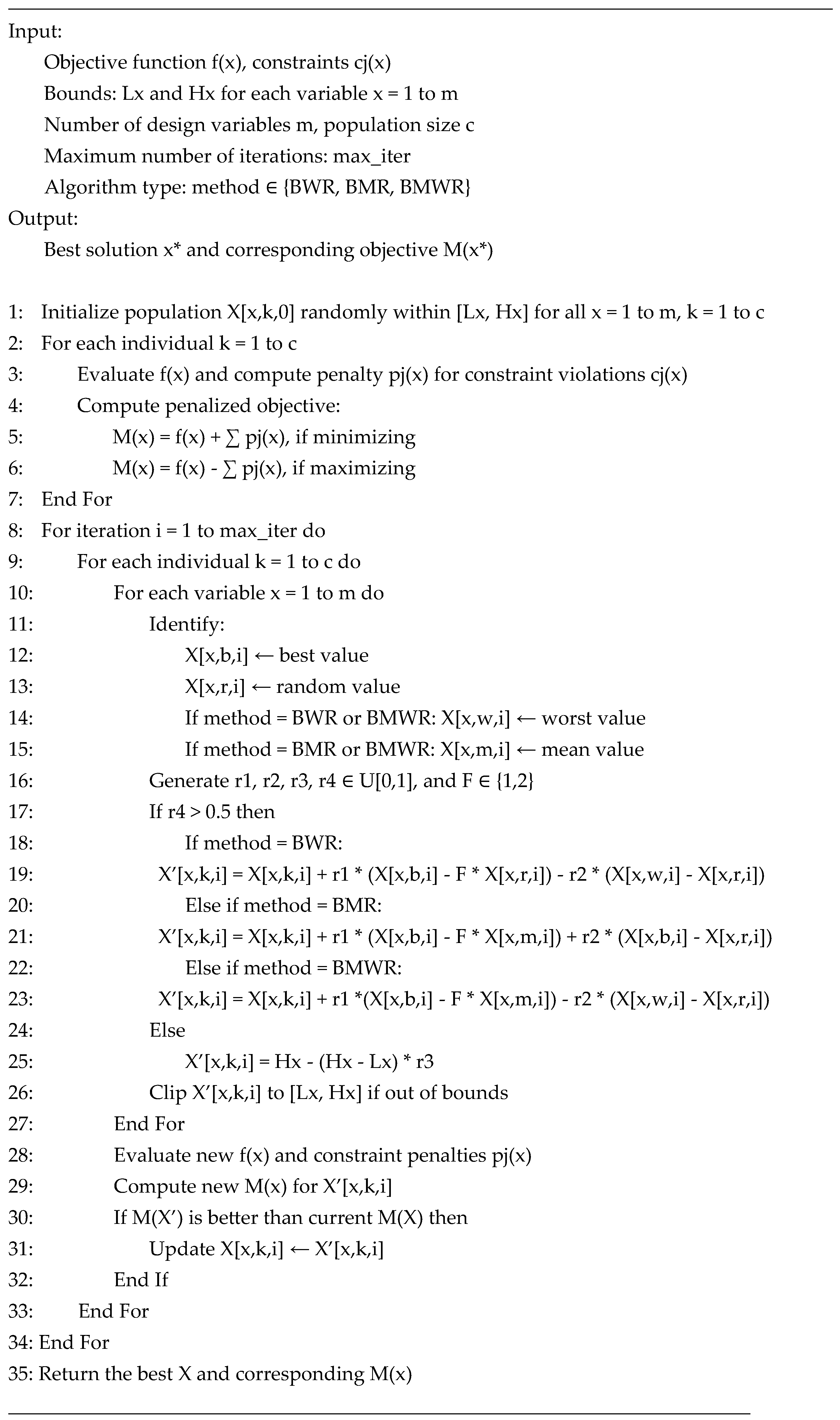
The unified pseudocode for the BWR, BMR, and the newly proposed BMWR algorithms is given in Figure 2.

2.1.4. Demonstration of the BWR, BMR, and BMWR Algorithms on a Constrained Benchmark Problem

Demonstration of the BWR Algorithm
To demonstrate the effectiveness and underlying mechanisms of the proposed BWR, BMR, and BMWR algorithms, a widely recognized benchmark problem is utilized. The constrained objective function is defined as Equation (5):
f(x): Minimize x12 + x22
Subject to the constraints given by Equations (6)–(8):
c1(x)= x1 + x2 − 1 ≤ 0
c2(x)= x1 − 0.2 ≥ 0
c3(x)= x2 − 0.3 ≥ 0
The variable bounds are given by Equation (9):
0 ≤ x1, x2 ≤1
The global minimum value for this constrained problem is known to be f(x) = 0.13 for x1 = 0.2 and x2 = 0.3.
Step 1: The objective function involves two design variables, x1 and x2. For demonstration purposes, a population size of 5 is used, with the termination criterion set at 1000 iterations. The randomly generated initial solutions are presented in Table 1.
Step 2: The optimal M(x) value of the objective function, considering the constraints, is determined and presented in Table 1. The corresponding best values of x1, x2, and M(x) are highlighted in bold, while the worst values of x1, x2, and M(x) are shown in italics.
Step 3: The optimal M(x) value of the objective function, subject to the constraints, corresponds to Solution 3, since the problem is formulated as a minimization task. Assume that the randomly generated numbers for x1 and x2 are r1 = 0.2, r2 = 0.4, and r3 = 0.2. These values are chosen solely for demonstration purposes; in actual implementation, the random numbers for x1 and x2 would be generated dynamically. The random number n4, generated during each iteration, determines whether Equation (1) or Equation (2) is used to update the values of x1 and x2. Assume that in the first iteration, r4 = 0.8, which is greater than 0.5. Therefore, Equations (1) and (2) are applied to modify x1 and x2. For example, in the first iteration, when Candidate Solution 1 randomly interacts with Candidate Solution 4, the updated values of x1 and x2 are calculated as follows:
X′x1,1,1 = 0.37454 + 0.2 ∗ (0.156019 − 1 ∗ 0.058084) − 0.4 ∗ (0.37454 − 0.058084) = 0.267545
X′x2,1,1 = 0.950714 + 0.2 ∗ (0.155995 − 1 ∗ 0.866176) − 0.4 ∗ (0.950714 − 0.866176) = 0.774863
The modified values of x1 and x2, along with the corresponding f(x), c1(x), p1, c2(x), p2, c3(x), p3, and M(x), are computed and presented in Table 2. In this iteration, the new x1 and x2 values for Candidate Solutions 1, 2, 3, 4, and 5 are obtained by considering Candidate Solutions 4, 5, 2, 3, and 1, respectively, as the random interaction partners.
Step 4: The updated M(x) values in Table 2 are compared with their corresponding previous M(x) values from Table 1 for the first iteration. The best M(x) values are retained, and the resulting population is presented in Table 3.
It is observed that, at the end of the first iteration, the best value is 0.071348 and the worst value is 0.706767, indicating an improvement in the worst solution compared to the randomly generated initial population.
Step 5: Based on the input from Table 3, the second iteration can be performed since the termination criterion has not been satisfied. However, the results of the second iteration are omitted here due to space limitations.
Step 6: Assuming the termination criterion of 1000 iterations is met, the final results at the end of the 1000th iteration are presented in Table 4.
It is evident that the proposed BWR algorithm achieves an optimum solution of 0.13, corresponding to the optimal values x1 = 0.2 and x2 = 0.3.
Demonstration of BMR Algorithm
To illustrate the proposed BMR optimization algorithm, the same constrained objective function is used. For performance comparison with the BWR algorithm, the initial population from Table 1 is retained, and the updated values of x1 and x2 are computed using Equation (3) (or Equation (2) if the updated values exceed the bounds). The mean values obtained from Table 1 are x1 = 0.3843504 and x2 = 0.6559216. Using the same random interactions as in the BWR algorithm—where candidate solutions 1–5 interact with 4, 5, 2, 3, and 1, respectively—the updated population is presented in Table 5. For instance, in the first iteration, when candidate solution 1 interacts with candidate solution 4 the modified values of x1 and x2 are computed using the BMR algorithm as follows.
X′x1,1,1 = 0.37454 + 0.2 ∗ (0.156019 − 1 ∗ 0.3843504) + 0.4 ∗ (0.156019 − 0.058084) = 0.368048
X′x2,1,1 = 0.950714 + 0.2 ∗ (0.155995 − 1 ∗ 0.6559216) + 0.4 ∗ (0.155995 − 0.866176) = 0.566656
The modified values are computed and are given in Table 5.
The modified M(x) values in Table 5 are compared with the corresponding M(x) values from Table 1 for the first iteration. The best M(x) values are retained, and the resulting population is presented in Table 6.
It can be seen that the best value at the end of the first iteration using the BMR algorithm is 0.071348 and the worst value is 0.622389. This shows the improvement in the worst solution compared to the randomly generated worst solution of 1.149928 given in Table 1.
Demonstration of BMWR Algorithm
Using Equations (2) and (4), the updated values of the variables, constraints, penalties, and objective function results obtained with the BMWR algorithm are presented in Table 7. For instance, in the first iteration, when candidate solution 1 interacts randomly with candidate solution 4 the modified values of x1 and x2 are computed using the BMWR algorithm as follows:
X′x1,1,1 = 0.37454 + 0.2 ∗ (0.156019 − 1 ∗ 0.3843504) − 0.4 ∗ (0.37454 − 0.058084) = 0.202291
X′x2,1,1 = 0.950714 + 0.2 ∗ (0.155995 − 1 ∗ 0.6559216) − 0.4 ∗ (0.950714 − 0.866176) = 0.816913
The modified values are computed and are given in Table 7.
Now the values of M(x) in Table 7 are compared with those in Table 1 and the best solutions are taken to form Table 8.
It is observed that, after the first iteration using the BMWR algorithm, the best value is 0.071348 and the worst value is 0.708638. This indicates an improvement in the worst solution compared to the initially generated worst value of 1.149928 presented in Table 1.
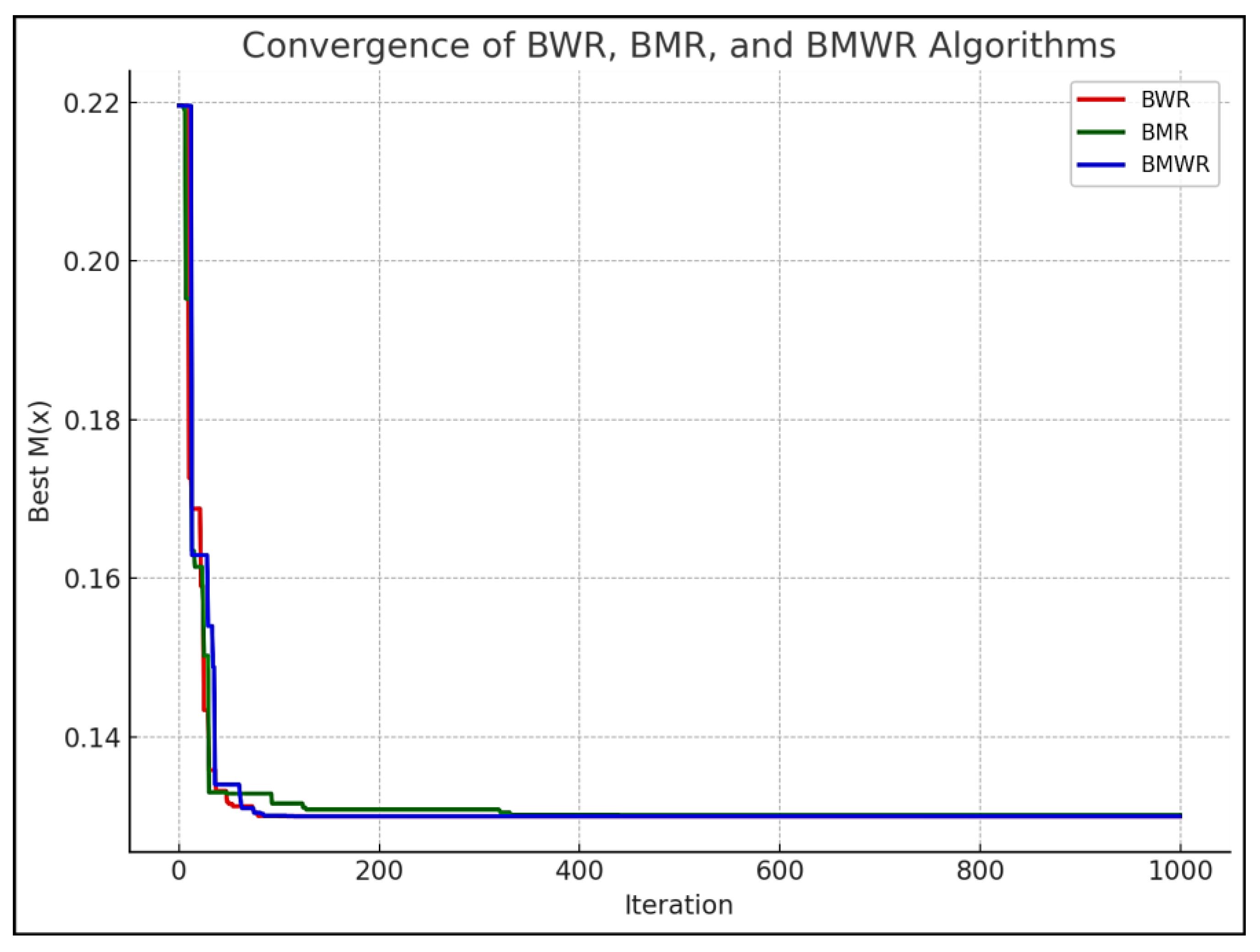
If the BWR, BMR, and BMWR algorithms are continued for 1000 iterations, then we can find that the global optimum value of f(x) = 0.13 for x1 = 0.2 and x2 = 0.3 is obtained. All the three algorithms converged to the same, as shown in Table 4. The convergence behaviors of the BWR, BMR, and BMWR algorithms are shown in Figure 3.
The trend for BWR for this constrained objective function is slower to converge compared to the other two, though it reaches the same final optimal value. The BMR algorithm shows efficient early performance and faster convergence. The BMWR algorithm showed best performance overall in terms of solution quality and convergence speed—reaching the feasible optimum with minimal fluctuation. The convergence occurred after 228, 312, and 207 iterations for the BWR, BMR, and BMWR algorithms, respectively.
Table 9 is presented below to present the novel features of the proposed BWR, BMR, and BMWR algorithms.

2.2. Proposed Algorithms for Multi-Objective Constrained Optimization Problems

This section outlines the multi-objective variants of the BWR, BMR, and BMWR algorithms. It also focuses on the multi-attribute decision-making (MADM) process used to select the most suitable compromise solution from the set of non-dominated Pareto-optimal solutions.

2.2.1. Multi-Objective Optimization with the BWR, BMR, and BMWR Algorithms

The extended versions of the BWR, BMR, and BMWR algorithms for handling multi-objective problems are referred to as MO-BWR, MO-BMR, and MO-BMWR, respectively. These algorithms incorporate several key features, including elite seeding, fast non-dominated sorting, constraint repair mechanisms, penalty application (when repair fails), local search enhancement, and edge-boosting strategies. A summary of the algorithmic procedure is provided in Table 10.
The total computational complexities of the MO-BWR, MO-BMR, and MO-BMWR algorithms are identical and given by O(I·(M.c2 + c·(m + tf + tp))), where M is the number of objectives, I is the number of iterations, c is the population size, m is the number of design variables, tf represents the time required to evaluate the objective functions and constraints per individual, and tp is the time needed for penalty computation (assumed proportional to the number of constraints). This complexity accounts for the quadratic cost associated with Pareto-based non-dominated sorting, and the linear cost associated with variable updates, evaluations, and penalties. The algorithms are well-suited for small to medium population sizes and can be made more scalable by incorporating faster sorting mechanisms such as those in NSGA-III. For the single-objective BWR, BMR, and BMWR algorithms, the total computational complexity is O(I·c·(m + tf + tp) as they do not involve non-dominated sorting. The only distinction between BWR, BMR, and BMWR lies in their update strategies, which does not impact their asymptotic complexity.

2.2.2. Validation of the MO-BWR, MO-BMR, MO-BMWR Algorithms for ZDT Functions

The standard Zitzler–Deb–Thiele (ZDT) benchmark functions are used to assess the performance of the proposed algorithms. A brief overview of these functions is presented below.
ZDT1:
f1(x) = x1
g(x) = 1 + 9 ∗ (1/(n − 1)) ∗ Σ xi for i = 2 to n
f2(x) = g(x) ∗ [1 − sqrt(f1(x)/g(x))]
ZDT2:
f1(x) = x1
g(x) = 1 + 9 ∗ (1/(n − 1)) ∗ Σ xi for i = 2 to n
f2(x) = g(x) ∗ [1 − (f1(x)/g(x))^2]
ZDT3:
f1(x) = x1
g(x) = 1 + 9 ∗ (1/(n − 1)) ∗ Σ xi for i = 2 to n
f2(x) = g(x) ∗ [1 − sqrt(f1(x)/g(x)) − (f1(x)/g(x)) ∗ sin(10π ∗ f1(x))]
ZDT4:
f1(x) = x1
g(x) = 1 + 10 ∗ (n − 1) + Σ [xi^2 − 10 ∗ cos(4π ∗ xi)] for i = 2 to n
f2(x) = g(x) ∗ [1 − sqrt(f1(x)/g(x))]
ZDT6:
f1(x) = 1 − exp(−4 ∗ x1) ∗ sin^6(6π ∗ x1)
g(x) = 1 + 9 ∗ (Σ xi for i = 2 to n)^(0.25)/(n − 1)
f2(x) = g(x) ∗ [1 − (f1(x)/g(x))^2]
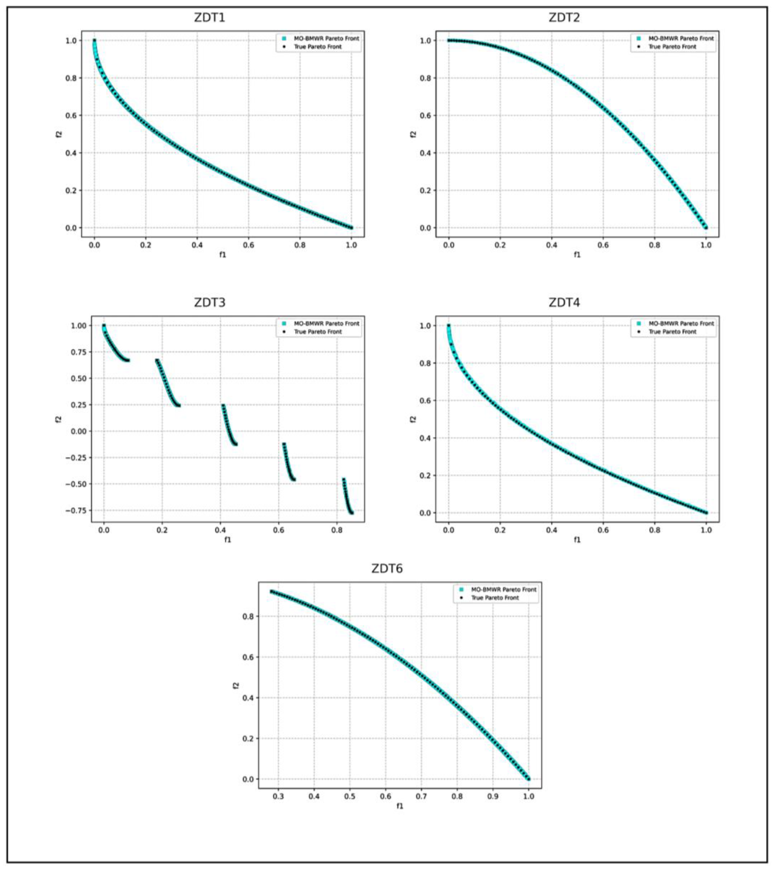
The MO-BWR, MO-BMR, and MO-BMWR algorithms are applied to the ZDT benchmark problems using 40,000 function evaluations. An equal number of function evaluations is used for performance comparison with the non-dominated sorting genetic algorithm III (NSGA-III) for each problem. Each experiment is executed 30 times. The implementations of MO-BWR, MO-BMR, and MO-BMWR are developed in Python 3.9 on a laptop equipped with an AMD Ryzen 5 5600H processor and 16 GB DDR4 RAM. The Pymoo library is utilized for benchmark problem definitions, their true Pareto fronts, and the NSGA-III algorithm. The results of algorithms on ZDT functions and the convergence graphs are given in Appendix A.
The MO-BWR, MO-BMR, and MO-BMWR algorithms have successfully addressed the standard Zitzler–Deb–Thiele (ZDT) multi-objective benchmark problems. Likewise, these algorithms can be extended to solve other multi-objective benchmark functions as well. However, prior studies have already demonstrated that the base versions have been effectively applied to a variety of standard benchmark problems [22] and complex engineering design tasks. The primary focus of this paper is to apply these algorithms to solve single- and multi-objective optimization problems encountered in metal casting processes.
It is important to note that Pareto-optimal solutions are non-dominated—meaning no solution is strictly better than another across all objectives—and each is considered acceptable. However, if a decision-maker wishes to prioritize certain objectives over others, a multi-attribute decision-making (MADM) approach can be employed. Numerous MADM methods have been proposed in the literature. Among them, a recent method called BHARAT, developed by Rao [23], offers a simple and logical approach to assigning relative importance to objectives and ranking the solutions accordingly.
The following sections present the application of the BWR, BMR, and BMWR algorithms for single-objective optimization of metal casting processes, followed by the use of MO-BWR, MO-BMR, and MO-BMWR for multi-objective optimization. Subsequently, the BHARAT method is applied to select the most preferred solution from the obtained set of Pareto-optimal alternatives.

3. Results and Discussion on the Application of the Proposed Algorithms for Optimizing Various Metal Casting Processes

Optimization of metal casting processes is critical due to the complex nature of casting operations, the variability of input parameters, and the cost-sensitive environment in which foundries operate. Casting involves numerous interdependent variables, such as mold design, gating and riser dimensions, pouring temperature, and cooling rate. Each of these factors significantly influences the quality, efficiency, and cost of the final product. Without optimization, achieving the desired quality consistently becomes a trial-and-error process, leading to high rates of scrap, rework, and energy consumption. Optimization of metal casting processes is essential for improving product quality, reducing costs, increasing efficiency, and ensuring consistency in production. It enables data-driven decision-making, minimizes reliance on empirical adjustments, and is an integral part of modern, sustainable manufacturing strategies. Now, optimization of different metal casting processes is presented in the following sub-sections.

3.1. Single-Objective Optimization of Metal Casting Processes

To demonstrate the applicability of the proposed BWR, BMR, and BMWR algorithms for single-objective optimization of metal casting processes, three case studies are examined.

3.1.1. Optimization of the Lost Foam Casting Process for Manufacturing a Fifth Wheel Coupling Shell from EN-GJS-400-18 Ductile Iron

Li et al. [12] optimized defect reduction in the lost foam casting process for producing a fifth wheel coupling shell. The semi-truck fifth wheel coupling, also known as the traction seat, is a vital chassis component that links the trailer to the truck. It locks onto the truck’s kingpin, ensuring a secure connection and enabling the transfer of horizontal and vertical forces between the truck and trailer. This component must also withstand dynamic loads and impacts encountered during various driving conditions, including starting, accelerating, braking, steering, and decelerating. The casting of the fifth wheel coupling considered by Li et al. [12] had dimensions of 916 mm × 760 mm × 140 mm, with a weight of approximately 126 kg. The shell featured an average wall thickness of 16 mm, reaching up to 20 mm at its thickest sections.
Manufactured from EN-GJS-400-18 ductile iron, the coupling benefits from this alloy’s notable ductility and toughness, setting it apart from other cast iron types. These properties make it ideal for applications that demand a balance between hardness and abrasion resistance. Consequently, it sees widespread use in industries such as marine, railways, transportation, wind energy, and various industrial machinery, especially in structural and safety-critical components. The casting process employed natural silica sand as the mold material and expanded polystyrene (EPS) foam as the pattern. EPS foam begins to decompose at approximately 290 °C; depending on the surface heat flux, it may fully vaporize into a gas or partially melt into a liquid phase.
Li et al. [12] designed a pouring system for the EN-GJS-400-18 ductile iron fifth wheel coupling shell, and ProCAST 2021 simulation software was used to simulate filling and solidification. Based on these simulations, risers were added in suitable positions to reduce casting defects. The Box–Behnken response surface methodology (RSM) using Design Expert 13 data processing software was applied to optimize three key process parameters: pouring temperature (A) in °C, pouring speed (B) in m/s, and ferro-static head pressure (C) in Pa. The process output parameter was the porosity (P) of the produced casting. The statistical tests of ANOVA and F-tests confirmed the best fitness and accuracy of the regression equation developed for P in terms of the process input parameters.
The optimum conditions were found to be a pouring temperature of 1386 °C, a pouring speed of 6.42 kg/s, and a ferrostatic head pressure of 109,751 Pa. Under these conditions, shrinkage was reduced, cracks were eliminated, and porosity decreased. With the optimized parameters, ProCAST predicted the locations of possible casting defects. Test castings were then produced, and samples were examined for metallographic structure and tensile properties. The results showed no major defects, and the casting quality met production and performance requirements.
The mathematical regression model for P in terms of the input parameters is given by Equation (25). The bounds of the input parameters are given in Equation (26).
Porosity (P) = 0.011 ∗ A + 0.746 ∗ B + 6.758 ∗ 10−6 ∗ C + 0.4 ∗ 10−4 ∗ A ∗ B + 8.520 ∗ 10−8 ∗ A ∗ C − 6.130 ∗ 10−6 ∗ B ∗ C − 7.308 ∗ 10−6 ∗ A2 − 0.014 ∗ B2 − 4.512 ∗ 10−10 ∗ C2
1350 °C ≤ A ≤ 1450 °C; 4.5 m/s ≤ B ≤ 6.5 m/s; 105,000 Pa ≤ C ≤ 110,000 Pa
Substituting the optimal values of A, B, and C suggested by Li et al. [12] into Equation (25) gives a porosity value of 9.82%!! Hence, the data from the 17 experiments given in Table 4 of the paper of Li et al. [12] is revisited and a correct regression model is formed. It is almost the same as Equation (25), but an important constant term of −8.856569 is added. The corrected regression model for the porosity P is written now as Equation (27).
Porosity (P) = −8.856569 + 0.010943 ∗ A + 0.745645 ∗ B + 6.758 ∗ 10−6 ∗ C + 0.4 ∗ 10−4 ∗ A ∗ B + 8.520 ∗ 10−8 ∗ A ∗ C − 6.130 ∗ 10−6 ∗ B ∗ C − 7.308 ∗ 10−6 ∗ A2 − 0.013845 ∗ B2 − 4.512 ∗ 10−10 ∗ C2
Substituting the optimal parameters of pouring temperature of 1386 °C, pouring speed of 6.42 kg/s, and ferro-static head pressure of 109,751 Pa, as suggested by Li et al. [12], into the corrected equation for porosity (i.e., Equation (27)) leads to a porosity of 0.792% (not 0.82%, as reported by Li et al. [12]).
Now to check if there can be any further improvement in the optimal values of A, B, and C, and the corresponding P, the proposed BWR, BMR, and BMWR algorithms are applied to the same regression model with the same bounds of the input parameters. A population size of 10 and 50 iterations are used, resulting in a total of 500 function evaluations. The results are presented in Table 11, with the best optimal porosity value highlighted in bold.
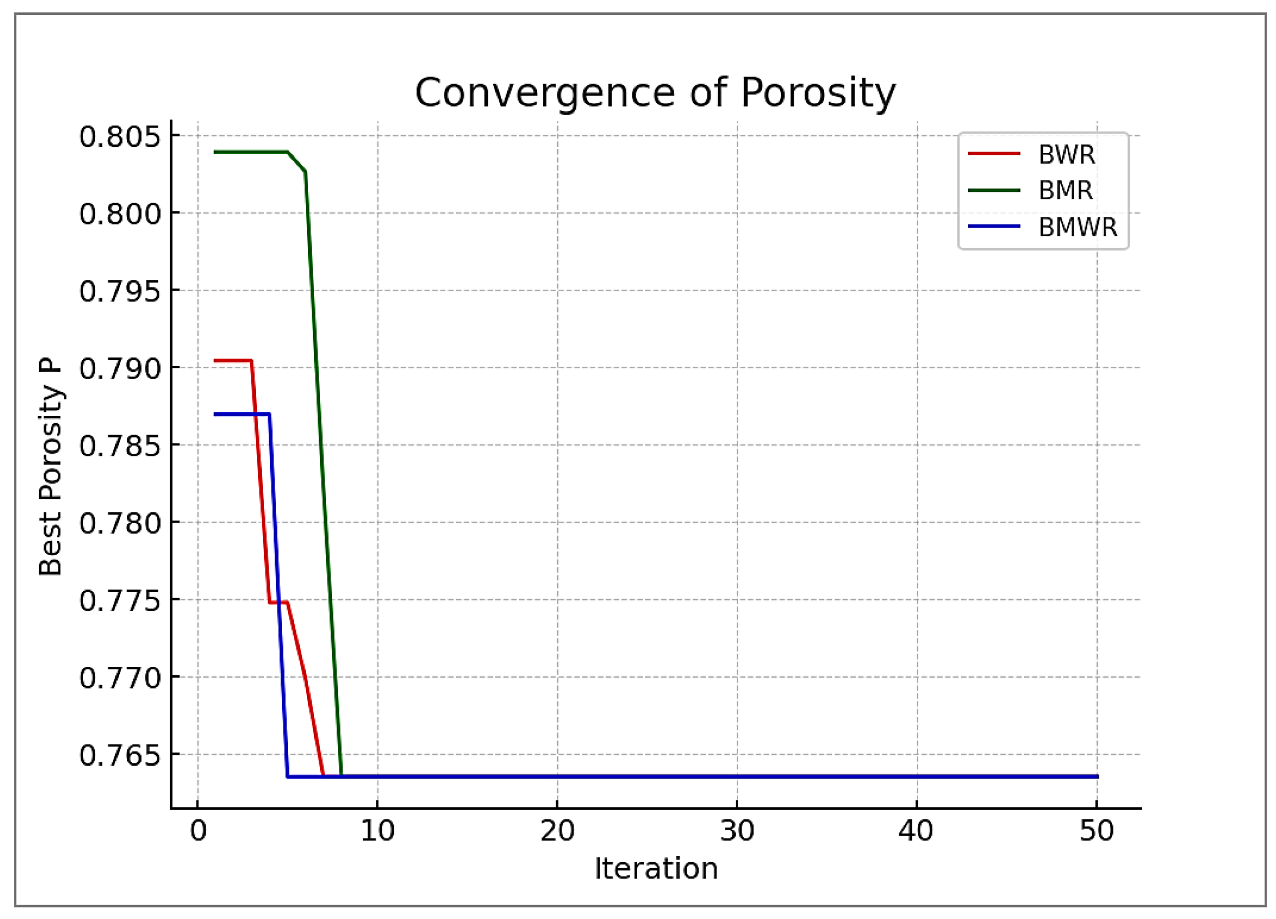
From Table 11, it can be understood that the BWR, BMR, and BMWR algorithms have produced a minimum porosity of 0.7635% compared to the 0.792% suggested by Li et al. [12] using RSM and ProCAST 2021 simulation software. It can also be seen that the BWR, BMR, and BMWR algorithms required only a few iterations to reach the optimal solution.
Figure 4 presents the convergence graphs of the BWR, BMR, and BMWR algorithms. The BMWR algorithm exhibits faster convergence, and all three algorithms achieve the global optimum value of f(x) = 0.7635 cm3. The convergence of the BMWR algorithm is faster and the BMR lagged slightly. BWR converged after the 7th iteration, BMR after the 8th iteration, and BMWR after the 5th iteration.
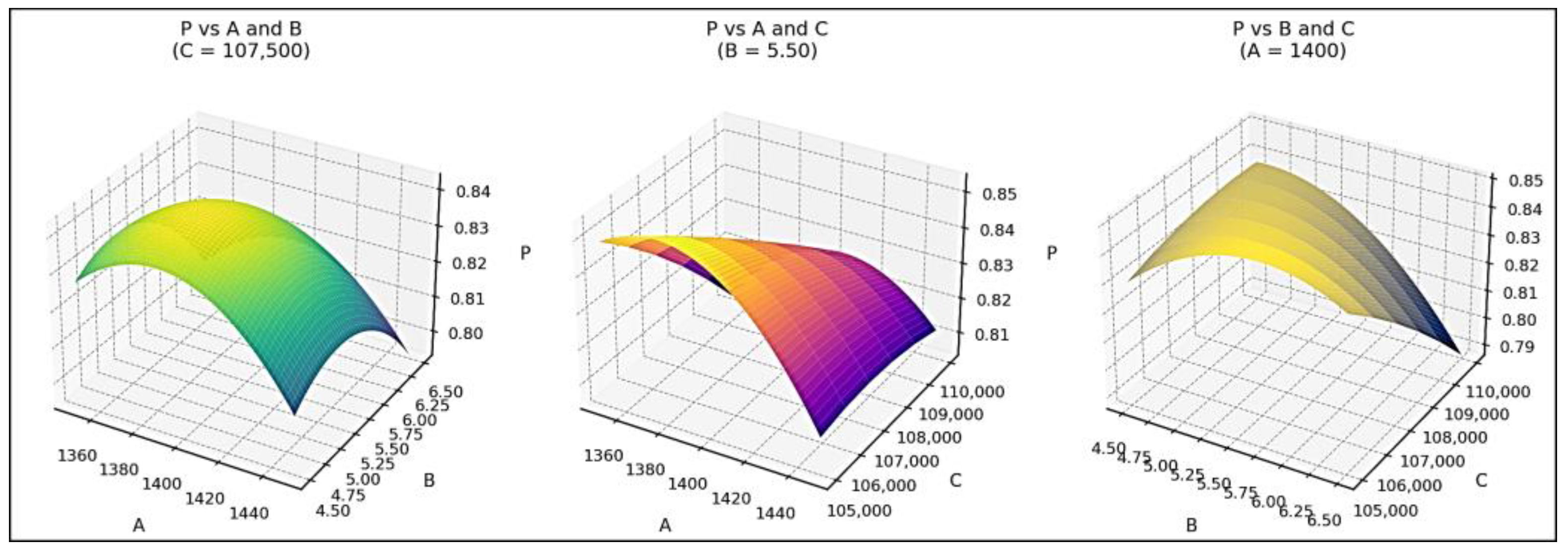
The effects of the input parameters A, B, and C on porosity P are shown in the surface plots shown in Figure 5.
In the above plot of P vs. A and B, the value of C is fixed at its mid-point of 107,500 Pa; in the plot of P vs. A and C, the value of B is fixed at its mid-point of 5.5 m/s; and in the plot of P vs. B and C, the value of A is fixed at its mid-point of 1400 °C. The surface plots reveal that higher values of both A and B reduce the porosity (when C is fixed at its mid-point); higher values of A and C reduce the porosity (when B is fixed at its mid-point); and higher values of B and C reduce the porosity (when A is fixed at its mid-point). Based on the regression equation of P, and taking into account the linear, quadratic, and interaction effects of the parameters, it can be concluded that parameter C is the most dominant, followed by B, and then A.

3.1.2. Optimization of Process Parameters of Die Casting of A360 Al-Alloy

Die casting is widely used for its high surface finish, dimensional accuracy, and cost-effectiveness, but it often suffers from a high defect rate, largely influenced by the gating system design. A360 Al-Alloy is commonly used and is considered a viable alternative to A380 Al-Alloy. Xu et al. [1] applied response surface methodology (RSM) based on the ordinary least squares (OLS) method to reduce severe defects in A360 Al-alloy cover plates arising from excessive porosity during die casting. The effects of three key process parameters—casting temperature (TC), mold preheating temperature (TM), and fast injection speed (V)—on volumetric porosity were systematically evaluated using 17 distinct combinations of injection molding settings. Optimal process parameters were determined and experimentally validated through RSM combined with computer-aided engineering (CAE) simulation. A 3D model of the cover plate casting, including the gating system, was developed using 3D modeling [1], and a chill vent was added and connected to the vacuum system.
The mathematical model developed for the volumetric porosity P is given by Equation (28). The statistical tests of ANOVA and F-tests confirmed the best fitness and accuracy of the regression equation developed for P in terms of the process input parameters. The bounds of the three critical process parameters—casting temperature (TC), mold preheating temperature (TM), and fast injection speed (V)—are given by Equation (29).
Volumetric porosity P (cm3) = −1.092681 + 0.012221 ∗ TC − 0.013113 ∗ TM − 0.919275 ∗ V −0.000012 ∗ TC2 + 0.00001 ∗ TC ∗ TM + 0.001485 ∗ TC*V + 0.000015 ∗ TM2 − 0.000462 ∗ TM ∗ V + 0.0104 ∗ V2
630 °C ≤ TC ≤ 670 °C; 180 °C ≤ TM ≤ 220 °C; 2.5 m/s ≤ V ≤ 3.5 m/s
Through RSM and CAE simulations, Xu et al. [1] reported the optimal values of TC, TM, and V as 630 °C, 220 °C, and 2.5 m/s. The volumetric porosity P obtained by substituting the optimal parameter values of TC, TM, and V in Equation (28) gives P as 0.9203 cm3 (not 0.8745 cm3 as incorrectly reported by Xu et al. [1]).
To explore potential improvements in the optimal values of TC, TM, and V, as well as the corresponding P, the proposed BWR, BMR, and BMWR algorithms are applied to the same regression model using identical input parameter bounds. A population size of 10 and 100 iterations are employed, resulting in 1000 function evaluations. Table 12 gives the comparison of optimal volumetric porosity P obtained in the die casting process for producing A360 Al-alloy cover plate. The best value of P is indicated in bold.
From Table 12, it can be understood that the BWR, BMR, and BMWR algorithms have produced a minimum volumetric porosity of 0.8995 cm3 compared to the 0.9203 cm3 produced by the RSM and CAE used by Xu et al. [1]. Xu et al. [1] reported the optimal porosity as 0.8745 cm3, corresponding to a casting temperature TC of 630 °C, a mold preheating temperature TM of 220 °C, and a fast injection speed V of 2.5 m/s. However, substituting those values of TC, TM, and V lead to a porosity value of 0.9203 cm3 (instead of 0.8745 cm3, as reported by Li et al. [12]).
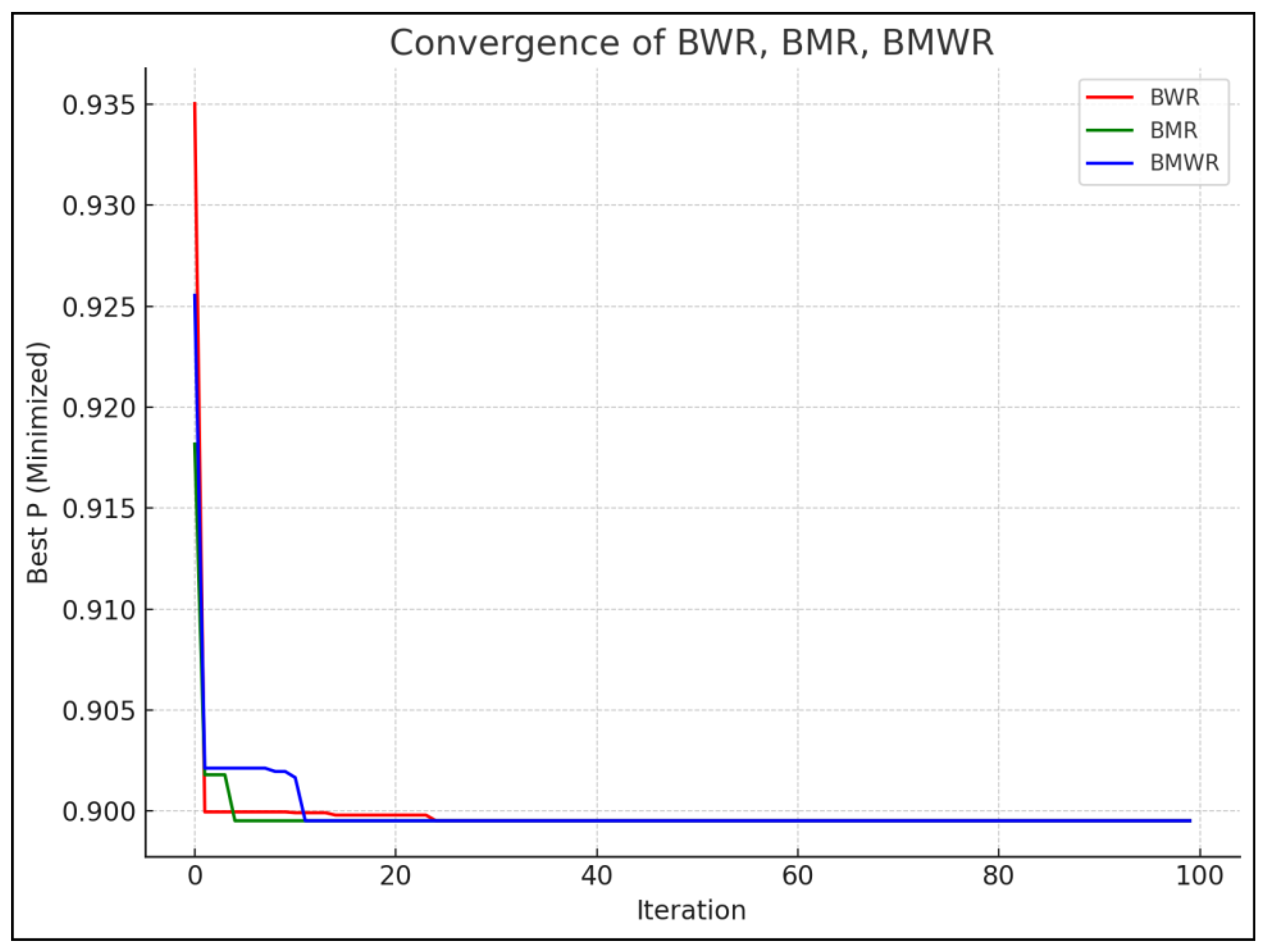
It can also be seen that the BWR, BMR, and BMWR algorithms required lower numbers of function evaluations to reach the optimal solution. Figure 6 shows the convergence graph of the BWR, BMR, and BMWR algorithms. The BWR algorithm showed best early convergence after 10 iterations, BMWR showed excellent stability and converged after 20 iterations, and BWR showed moderate stability and converged after the 25th iteration. All three algorithms (BWR, BMR, and BMWR) converged to the same optimum value of volumetric porosity P, which was 0.8995 cm3.
Figure 7 presents three surface plots illustrating the effects of casting temperature (TC), mold temperature (TM), and injection speed (V) on porosity (P).
In the above plot of P vs. TC and TM, the value of V is fixed at its mid-point of 3.0 m/s; in the plot of P vs. TC and V, the value of TM is fixed at its mid-point of 200 °C; and in the plot of P vs. TM and V, the value of TC is fixed at its mid-point of 650 °C. The surface plots reveal that lower TC and lower TM reduces the porosity (when V is fixed at its mid-point); lower TC and lower V reduces the porosity (when TM is fixed at its mid-point); and lower TM and lower V reduces the porosity (when TC is fixed at its mid-point). Based on the regression equation of P, and taking into account the linear, quadratic, and interaction effects of the parameters, it can be concluded that parameter TC is the most dominant, followed by TM, and then V.

3.1.3. Optimization of Wear Rate of an AA7178 Alloy Reinforced with Nano-SiC Particles Produced Using a Stir-Casting Process

Metal matrix composites (MMCs) are increasingly replacing traditional materials due to their superior mechanical and tribological properties. Ceramic nanoparticle reinforcements like SiC, TiO2, Al2O3, ZrB2, and TiC have shown great potential in aerospace, automotive, and biomedical applications. However, optimizing their wear behavior is challenging due to complex interactions among process parameters. While methods like response surface methodology (RSM) and Taguchi have been used, they struggle with nonlinear relationships. Metaheuristic optimization techniques offer a more effective alternative by efficiently handling complex, multi-parameter problems and identifying global optima. This has positioned metaheuristic approaches as valuable tools for advancing the performance and reliability of these advanced composite materials.
Bharat et al. [5] investigated the microstructure and wear behavior of AA7178 alloy reinforced with varying weight percentages (0, 1, 2, and 3%) of nano-SiC particles, fabricated via stir casting, to improve material performance under wear conditions. It addressed limitations in current aerospace materials, which often exhibit poor wear resistance, surface degradation, and reduced durability under abrasive environments—factors that lead to higher maintenance costs and decreased operational efficiency. AA7178 alloy was first dried in a muffle furnace at 450 °C for 45 min to remove moisture and impurities, then melted in a graphite crucible. Nano-SiC particles were added to the melt and stirred at 625 rpm for 10–15 min for uniform dispersion. Magnesium powder was introduced to improve wettability and reduce surface tension. The final slurry was poured into a preheated permanent iron mold.
The research hypothesized that incorporating nano-SiC into the AA7178 matrix would enhance wear resistance and contribute to the development of high-performance metal matrix composites. To evaluate this, dry sliding wear tests were performed using a pin-on-disk apparatus. Experiments were systematically varied across sliding velocity A (1–4 m/s), sliding wear distance B (500–2000 m), applied load C (9.81–39.24 N), and weight % of nano-SiC (0–3%). The L16 Taguchi design was used to plan and analyze the experiments in terms of the signal-to-noise ratio. To analyze the influence of process factors, Minitab 18 software was used, and ANOVA was performed to evaluate the relative importance of each parameter. The RSM model was used to predict the wear rate, given by Equation (30). The coefficient of determination (i.e., R2) was 99.88%, which indicates the best fit with highest accuracy. The bounds of the process input parameters are given by Equation (31):
Wear rate ((mm3/m) ∗ 10−3) = 2.381 − 0.106 ∗ A + 0.000657 ∗ B + 0.0357 ∗ C −0.353 ∗ D + 0.01004 ∗ A ∗ C + 0.00418 ∗ C ∗ D − 0.000012 ∗ C ∗ B − 0.0160 ∗ A ∗ D − 0.000061 ∗ A ∗ B − 0.000008 ∗ D ∗ B
1 m/s ≤ A ≤ 4 m/s, 500 m ≤ B ≤ 2000 m, 9.81 N ≤ C ≤ 39.24 N, and 0% ≤ D ≤ 3%
Bharat et al. [5] employed three metaheuristic algorithms—particle swarm optimization (PSO), artificial bee colony (ABC), and Rao-1—to determine the optimal values of AAA, BBB, CCC, and DDD. Using a population size of 50 and 50 iterations, they performed a total of 2500 function evaluations. To demonstrate the efficiency of the proposed BWR, BMR, and BMWR algorithms, a smaller population size of 10 and 50 iterations was used, resulting in only 500 function evaluations. The wear rate values obtained by the different algorithms are presented in Table 13, with the best optimal wear rate highlighted in bold.
The optimum value of wear loss (i.e., f(x)) obtained by the BMR, BWR, and BMWR algorithms is f(x) = 1.7088 × 10⁻³ mm3/m, with the optimal values of A = 4 m/s, B = 500 m, C = 9.81 N, and D = 3%. The value of wear loss obtained by the Rao-1 algorithm used by Bharat et al. [5] was also 1.7088 ∗ 10−3 mm3/m. The optimum values obtained by Bharat et al. [5] using the ABC and PSO algorithms are not optimal. Unlike the ABC and PSO algorithms, the BMR, BWR, BMWR, and Rao-1 algorithms do not need to tune any algorithm-specific parameters. Furthermore, as can be seen in this example, compared to the Rao-1 algorithm, the BWR, BMR, and BMWR algorithms required a smaller number of function evaluations to reach the optimal solution.
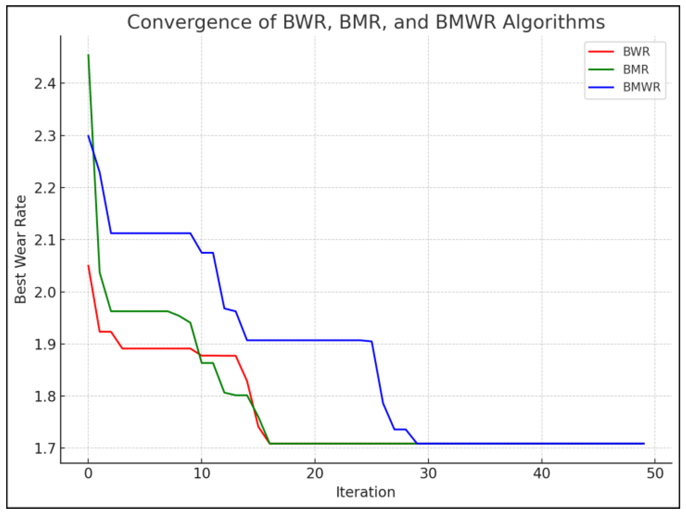
Figure 8 presents the convergence graph of the BWR, BMR, and BMWR algorithms. The BWR algorithm demonstrates faster convergence, and all three algorithms achieve a global optimum value of f(x) = 1.7088 × 10⁻³ mm3/m.
The BWR and BMR are faster and more efficient for this problem, converging quickly. The convergence occurred from the 16th iteration. The BMWR offers a balance of exploration and exploitation, but at the cost of slower convergence. The convergence occurred from the 29th iteration. If robustness in avoiding local optima is important, BMWR may be better suited despite slower convergence. The surface plots showing the effect of the input variables A, B, C, and D on wear rate are shown in Figure 9.
In the above plot of wear rate vs. A and B, the values of C and D are fixed at their mid-point values of 24.53 N and 1.5%, respectively; in the plot of wear rate vs. A and C, the values of B and D are fixed at their mid-point values of 1250 m and 1.5%, respectively; in the plot of wear rate vs. A and D, the values of B and C are fixed at their mid-point values of 1250 m and 24.53 N, respectively; in the plot of wear rate vs. B and C, the values of A and D are fixed at their mid-point values of 2.5 m/s and 1.5%, respectively; in the plot of wear rate vs. B and D, the values of A and C are fixed at their mid-point values of 2.5 m/s and 24.53 N, respectively; and in the plot of wear rate vs. C and D, the values of A and D are fixed at their mid-point values of 2.5 m/s and 1250 m, respectively.
It is observed that the wear rate decreases with higher speed and shorter distance; increases with rising load (C) and decreases with increasing speed (A); and drops significantly with higher nano-SiC content (%) combined with increased speed. Furthermore, wear rate increases with load; wear rate decreases with higher D (nano-SiC) and lower B (distance); and wear rate increases with load (C) but decreases with nano-SiC (D). The speed (A) and nano-SiC (D) are the most beneficial parameters for reducing wear. The load (C) and distance (B) are the most detrimental if increased. Higher values of A and D help reduce wear rate.

3.2. Multi-Objective Optimization of Metal Casting Processes

Multi-objective optimization (MOO) refers to the simultaneous optimization of two or more conflicting objectives. In metal casting, these objectives may include:
  • Minimizing porosity;
  • Minimizing shrinkage defects;
  • Minimizing solidification time;
  • Maximizing mechanical properties (e.g., hardness, tensile strength);
  • Reducing production costs.
MOO uses concepts such as Pareto-optimality to identify a set of optimal solutions, each representing a different trade-off scenario. This allows process engineers to select the most suitable solution based on specific constraints or priorities. The MOO allows balancing between competing objectives, provides a Pareto front offering flexibility in decision-making, helps in understanding how process parameters affect multiple outputs simultaneously, and the solutions are typically more resilient to parameter variations and uncertainties.
To demonstrate the applicability of the proposed BWR, BMR, and BMWR algorithms for multi-objective optimization of metal casting processes, two case studies are examined.

3.2.1. Multi-Objective Optimization of a Low-Pressure Casting Process Using a Sand Mold for Producing A356 Engine Block

Deng et al. [4] optimized the process parameters of a low-pressure casting process using a sand mold that was used for producing a four-cylinder A356 alloy engine block weighing 18.83 kg with the dimensions of 371.5 × 348.7 × 282.6 mm. The casting must be free from cold segregation, cracks, underpouring, sand burn-on, and shrinkage defects. Deng et al. [4] carried out multi-objective optimization of A356 engine block casting parameters using response surface methodology (RSM) in combination with the NSGA-II algorithm. Their study optimized the low-pressure casting process of A356 alloy engine blocks by analyzing four key parameters: pouring temperature A (°C), mold preheating temperature B (°C), filling time C (s), and holding pressure D (kPa). Using RSM and the NSGA-II algorithm through 29 test runs, two objectives were optimized—solidification time Y1 (s) and shrinkage volume Y2 (cm3). Both Y1 and Y2 are to be minimized. The mathematical regression models for Y1 and Y2 are given by Equations (32) and (33). The statistical tests of ANOVA and F-tests confirmed the best fitness and accuracy of the regression equations developed for Y1 and Y2 in terms of the process input parameters. The bounds of the process parameters are given by Equation (34).
Solidification time Y1 (s) = 3227.71435 − 10.52667 ∗ A + 0.519167 ∗ B + 66.25 ∗ C
+ 0.300926 ∗ D − 0.001438 ∗ A ∗ B − 0.07175 ∗ A ∗ C − 0.0005 ∗ A ∗ D + 0.0235 ∗ B ∗ C + 0.00825 ∗ B ∗ D + 0.004667 ∗ C ∗ D + 0.009823 ∗ A2 − 0.00049 ∗ B2 − 0.474333 ∗ C2 − 0.003259 ∗ D2
Shrinkage volume Y2 (cm3) = 246.25699 − 0.488750 ∗ A − 0.243250 ∗ B − 1.29817 ∗ C + 0.487481 ∗ D + 0.0004 ∗ A ∗ B + 0.00135 ∗ A ∗ C − 0.000742 ∗ A ∗ D + 0.00145 ∗ B ∗ C − 0.0007 ∗ B ∗ D − 0.002333 ∗ C ∗ D + 0.000354 ∗ A2 − 0.000049B2 + 0.015417 ∗ C2 + 0.000674D2
680 °C ≤ A ≤ 720 °C, 20 °C ≤ B ≤ 60 °C, 10 s ≤ C ≤ 20 s, and 50 kPa ≤ D ≤ 80 kPa
Deng et al. [4] used the NSGA-II algorithm and proposed the optimal values of parameters as pouring temperature A = 680 °C, mold preheat B = 20 °C, filling time C = 12 s, and pressure D = 50 kPa. Furthermore, using finite element analysis (FEA) simulation, Deng et al. [4] proposed the optimal values of Y1 as 745 s and Y2 as 74.25 cm3. The corresponding process input parameters obtained using FEA were not reported by Deng et al. [4].
Now, to explore potential improvements in the optimal sets of values of the parameters A–D and the corresponding non-dominated Pareto solutions the proposed MO-BWR, MO-BMR, and MO-BMWR algorithms are applied to the same regression models given by Equations (32) and (33), using identical input parameter bounds given by Equation (34). A population size of 50 and 200 iterations are employed, resulting in 10,000 function evaluations (same as those used by NSGA-II in [4]).
Before applying the MOO versions, BWR, BMR, and BMWR are applied to the individual objective functions individually to discover the best optimal values of solidification time Y1 and shrinkage volume Y2.
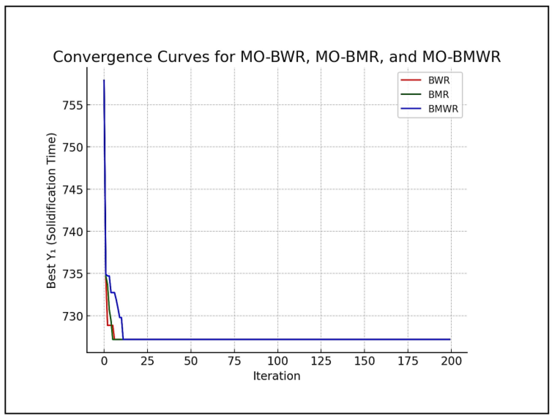
  • All three algorithms have given the best minimum value of Y1 as 727.18127 s, corresponding to A = 680 °C, B = 20 °C, C = 10 s, and D = 80 kPa. The convergence graphs are shown in Figure 10.
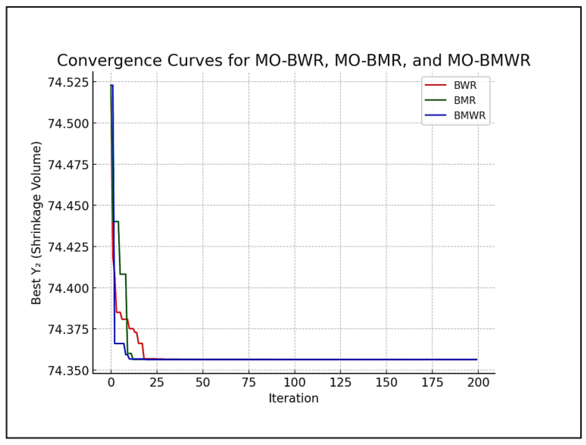
  • Similarly, all three algorithms have given the best minimum value of Y2 as 74.3563 cm3, corresponding to A = 720 °C, B = 20 °C, C = 15.01 s, and D = 71.057 kPa. The convergence graphs are shown in Figure 11.
However, in actual practice, both the objective functions Y1 and Y2 have to be attempted simultaneously to find the real optimum values of variables. For this purpose, the MO-BWR, MO-BMR, and MO-BMWR algorithms are applied to find out the optimum values of parameters A–D. Deng et al. [4] used the NSGA-II algorithm with a population size of 50 and number of iterations of 200 (i.e., function evaluations = 50 ∗ 200 = 10,000).
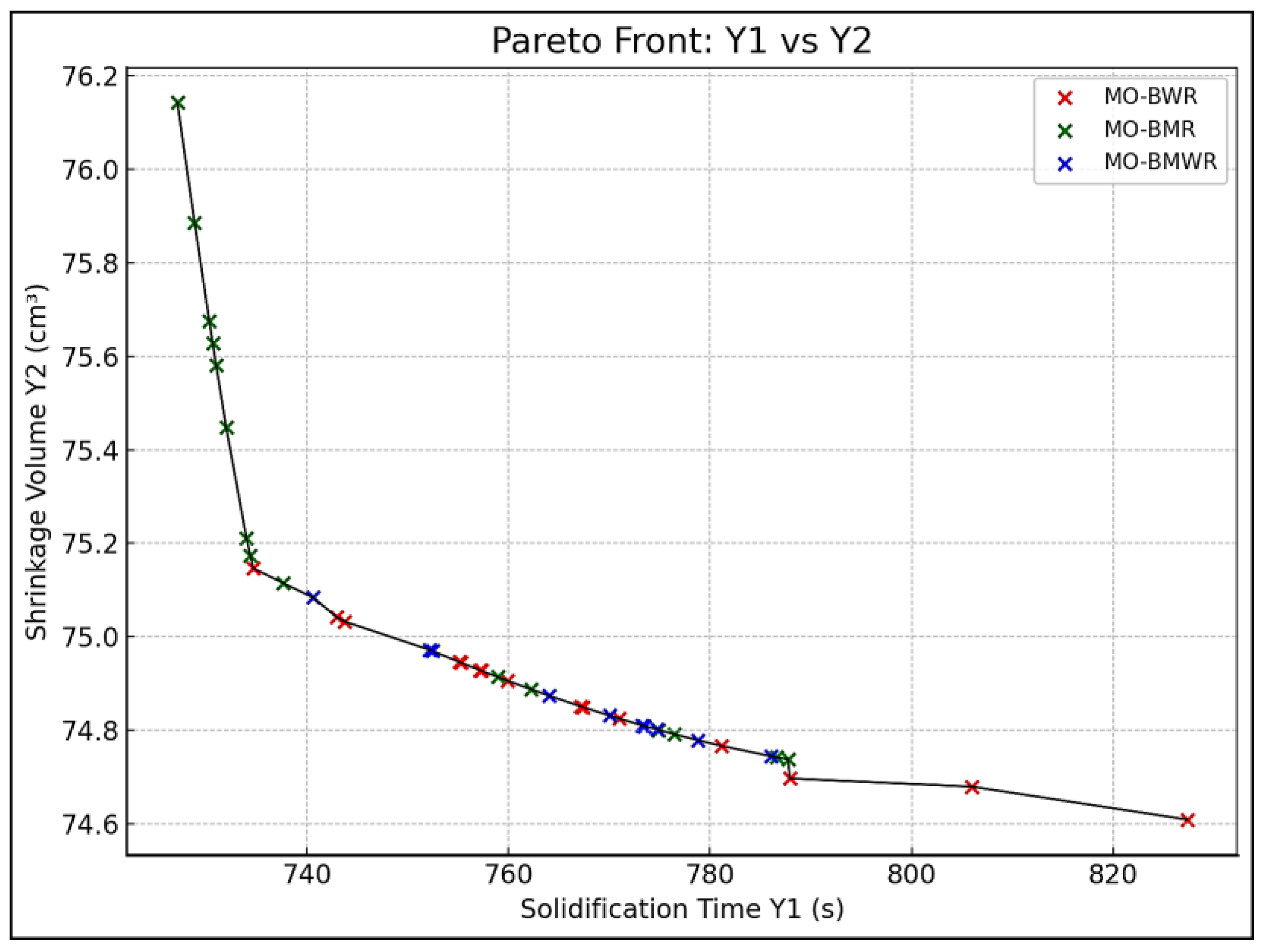
Now the proposed three algorithms are applied with the same number of function evaluations. The non-dominated Pareto-optimal solutions obtained are combined to form the composite front. The composite front contains 40 unique, non-repeating, non-dominated solutions. These 40 Pareto-optimal solutions are formed with MO-BMR’s 15 solutions, MO-BMWR’s 10 solutions, and MO-BWR’s 10 solutions. Table 14 shows the performance metrics of the three algorithms with reference to the composite front.
The MO-BMWR outperforms in IGD (0.032764) and has the highest hypervolume (0.731088) among the individual algorithms, indicating high-quality and well-spread solutions. The MO-BMR achieves the lowest spacing (0.021535), meaning its solutions are very evenly distributed. The MO-BWR lags behind in IGD and hypervolume, suggesting less extensive and less representative coverage. The composite front shows the best hypervolume and perfect IGD, as expected since it is the reference.
The composite Pareto front represents a non-dominated frontier obtained by merging the elite-boosted runs, providing the best trade-off solutions derived from the strategies of all three algorithms. Table 15 presents the set of 40 unique non-dominated optimal solutions produced by the three algorithms, after eliminating all duplicate solutions.
The metal casting process planners or decision-makers can select a point from the Pareto front based on their preference or constraints, e.g., if cycle time is critical, they can pick a point with lower Y1 even if Y2 is slightly higher. If defect minimization is more important, choose a solution with lower Y2 even if Y1 increases.
Figure 12 presents the non-dominated Pareto solutions of the composite front.
Now, the BHARAT method [23] is applied to find the best compromise Pareto-optimal solution out of the 29 non-dominated solutions of the composite front obtained by the combination of MO-BWR, MO-BMR, and MO-BMWR. The objectives values of Y1 and Y2 are normalized and shown in Table 15. As lower values are desired for both Y1 and Y2, the best values of Y1 and Y2 (i.e., Y1best = 727.1813 and Y2best = 74.60873, respectively) are taken from Table 15. The other values are normalized as Yjnormalized = Yibest/Yj. For example, the normalized values of Y1 and Y2 for solution no. 1 are 0.989748 (=727.1813/734.7135) and 0.992843 (=74.60873/75.14654), respectively. Similarly, the values of Y1 and Y2 are normalized for the other solutions.
If the decision-maker gives equal importance to both objectives Y1 and Y2 (i.e., wᵧ1 = wᵧ2), then each objective is assigned an average rank of 1.5 (the mean of ranks 1 and 2). Based on the reference table provided in [23], the BHARAT method assigns an equal weight of 0.5 to each objective for the rank of 1.5. The corresponding scores (weighted sums) are presented in the second-last column in Table 15. For example, the score for solution no. 1 is calculated as 0.5 ∗ 0.989748 + 0.5 ∗ 0.992843 = 0.991296. It is clear from the scores of the solution given in Table 15 that solution 1 is the best Pareto solution.
Table 16 makes a comparison of the optimization results. The best values of Y1 and Y2 are indicated in bold. The composite front has given a number of trade-off solutions and five of the such top solutions are included in Table 16.
It may be observed that the proposed algorithms have given trade-off solutions, and five of the top solutions given in Table 16 give a much better minimum solidification time Y1 compared to the NSGA-II and finite element simulation of Deng et al. [4]. The optimum shrinkage volume given by the proposed algorithms is also reasonable compared to the solutions given by Deng et al. [4]. In fact, Deng et al. [4] did not provide the values of the input parameters to check the values of Y1 and Y2 reported by them.
This example validates the proposed MO-BWR, MO-BMR, and MO-BMWR algorithms for the multi-objective optimization of the low-pressure casting process.
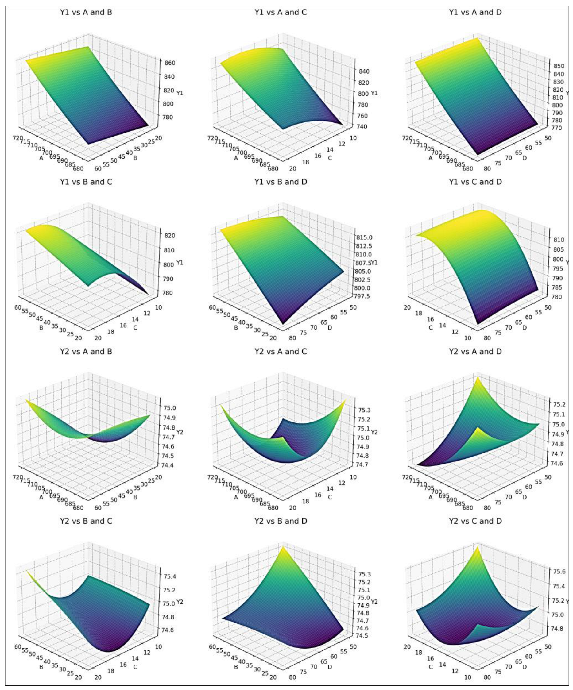
The surface plots showing the effects of the process parameters A, B, C, and D on Y1 and Y2 are shown in Figure 13. The 12 surface plots are arranged in four rows, with 3 plots per row, showing the effect of all pairwise combinations of A, B, C, and D on Y1 (solidification time) and Y2 (shrinkage volume).
In the above plot of solidification time Y1 vs. A and B, the values of C and D are fixed at their mid-point values of 15 s and 65 kPa, respectively. In the plot of Y1 vs. A and C, the values of B and D are fixed at their mid-point values of 40 °C and 65 kPa, respectively. In the plot of Y1 vs. A and D, the values of B and C are fixed at their mid-point values of 40 °C and 15 s, respectively. In the plot of Y1 vs. B and C, the values of A and D are fixed at their mid-point values of 700 °C and 65 kPa, respectively. In the plot of Y1 vs. B and D, the values of A and C are fixed at their mid-point values of 700 °C and 15 s, respectively. In the plot of Y1 vs. C and D, and the values of A and D are fixed at their mid-point values of 700 °C and 65 kPa, respectively. Similar fixing of the variables A, B, C, and D is performed for the plots of shrinkage volume Y2 versus the variables.
The surface plots reveal distinct and consistent trends in how the input parameters A–D influence the outputs Y1 (solidification time) and Y2 (shrinkage volume). For Y1, solidification time generally increases with higher values of C (filling time) and A (pouring temperature), indicating their dominant influence. The roles of B and D are more moderate but still positive, suggesting a cumulative effect when all variables are high. Conversely, Y2 (shrinkage volume) exhibits a more complex behavior. It tends to decrease with increasing C and D, indicating their effectiveness in minimizing shrinkage. There is a subtle curvature with respect to A and B, suggesting optimal intermediate values rather than extreme high or low settings. Overall, reducing Y2 while keeping Y1 low appears to require careful balancing—especially increasing C and D while avoiding excessively high A and B. The nonlinearity and interaction effects across the plots highlight the importance of multi-objective optimization for effective process parameter tuning.

3.2.2. Multi-Objective Optimization of a Squeeze Casting Process for LM20 Material

Optimizing squeeze casting parameters is vital for producing high-quality, low-cost castings, though limited studies exist. Patel et al. [11] carried out squeeze casting of LM20 aluminum alloy. LM20 alloy was selected for its excellent fluidity, pressure tightness, and resistance to hot tearing, wear, and corrosion, making it ideal for marine, automotive, engineering, and domestic applications. H13-grade chromium–molybdenum heat-treated steel was used for making the die. After cleaning and degassing, the molten metal was poured into a preheated die, pressed until solidification, then released and removed from the die. The squeeze casting process parameters considered were as follows: time delay (Td) in seconds, pressure duration (Dp) in seconds, squeeze pressure (Sp) in MPa, pouring temperature (Pt) in °C, and die temperature (Dt) in °C.
Patel et al. [11] employed statistical tools to develop nonlinear regression models and identify the significant effects of squeeze casting process parameters on surface roughness (Ra), hardness (H), yield strength (YS), and ultimate tensile strength (UTS) of the produced parts. The accuracy of these models was validated using ten test cases, showing that they could predict the responses with high reliability. The resulting mathematical input–output relationships offered practical guidance for foundry operators to make more accurate process predictions. This study addressed the four inherently conflicting objectives of Ra, H, YS, and UTS, which were mathematically formulated into a single objective function. The widely used evolutionary genetic algorithm (GA) was then applied to determine the optimal process parameters. Multi-objective optimization was performed using the evolutionary genetic algorithm (GA). The optimization was conducted by assigning different weights to the responses, resulting in a set of optimal process parameters determined according to the assigned priorities.
Now to demonstrate and validate the proposed BWR, BMR, and BMWR algorithms, the squeeze casting process parameters case study presented by Patel et al. [11] is considered to see if there can be any further improvement in the optimal solutions. The four objective functions (i.e., output responses) are described by Equations (35)–(38). The bounds of the process input parameters are given by Equation (39). These are all as follows:
Surface roughness Ra (μm) = 19.4116 − 0.0933924 ∗ Td − 0.0170929 ∗ Dp− 0.0124204 ∗ Sp − 0.0437485 ∗ Pt − 0.00421634 ∗ Dt+ 0.0109566 ∗ Td2 + 0.000107382 ∗ Dp2+ 3.40018E − 05 ∗ Sp2 + 2.85979E − 05 ∗ Pt2+ 6.76585E − 06 ∗ Dt2
Yield strength YS (MPa) = − 879.007 + 0.100644 ∗ Td+ 0.616749 ∗ Dp + 0.627314 ∗ Sp+ 2.53574 ∗ Pt + 0.610584 ∗ Dt− 0.189332 ∗ Td2 − 0.00727915 ∗ Dp2− 0.0020318 ∗ Sp2 − 0.00178919 ∗ Pt2− 0.00132646 ∗ Dt2
Ultimate tensile strength UTS (MPa) = −1414.09 − 5.86888 ∗ Td + 1.31391 ∗ Dp+ 0.815477 ∗ Sp + 4.15593 ∗ Pt+ 0.887826 ∗ Dt + 0.119206 ∗ Td2− 0.0152318 ∗ Dp2 − 0.00243251 ∗ Sp2− 0.00293425 ∗ Pt2 − 0.00184456 ∗ Dt2
Hardness H (BHN) = − 283.664 − 1.09353 ∗ Td + 0.214051 ∗ Dp+ 0.307208 ∗ Sp + 0.87264 ∗ Pt+ 0.208767 ∗ Dt − 0.0254625 ∗ Td2 − 0.00190085 ∗ Dp2 − 9.35689 ∗ E − 04 ∗ Sp2− 6.03363E − 04 ∗ Pt2 − 3.81916E − 04 ∗ Dt2
3 s ≤ Td ≤ 11 s, 10 s ≤ Dp ≤ 50 s, 0.1 MPa ≤ Sp ≤ 200 MPa, 630 °C ≤ Pt ≤ 750 °C, 100 °C ≤ Dt ≤ 300 °C
The Ra is to be minimized and the YS, UTS, and H are to be maximized.
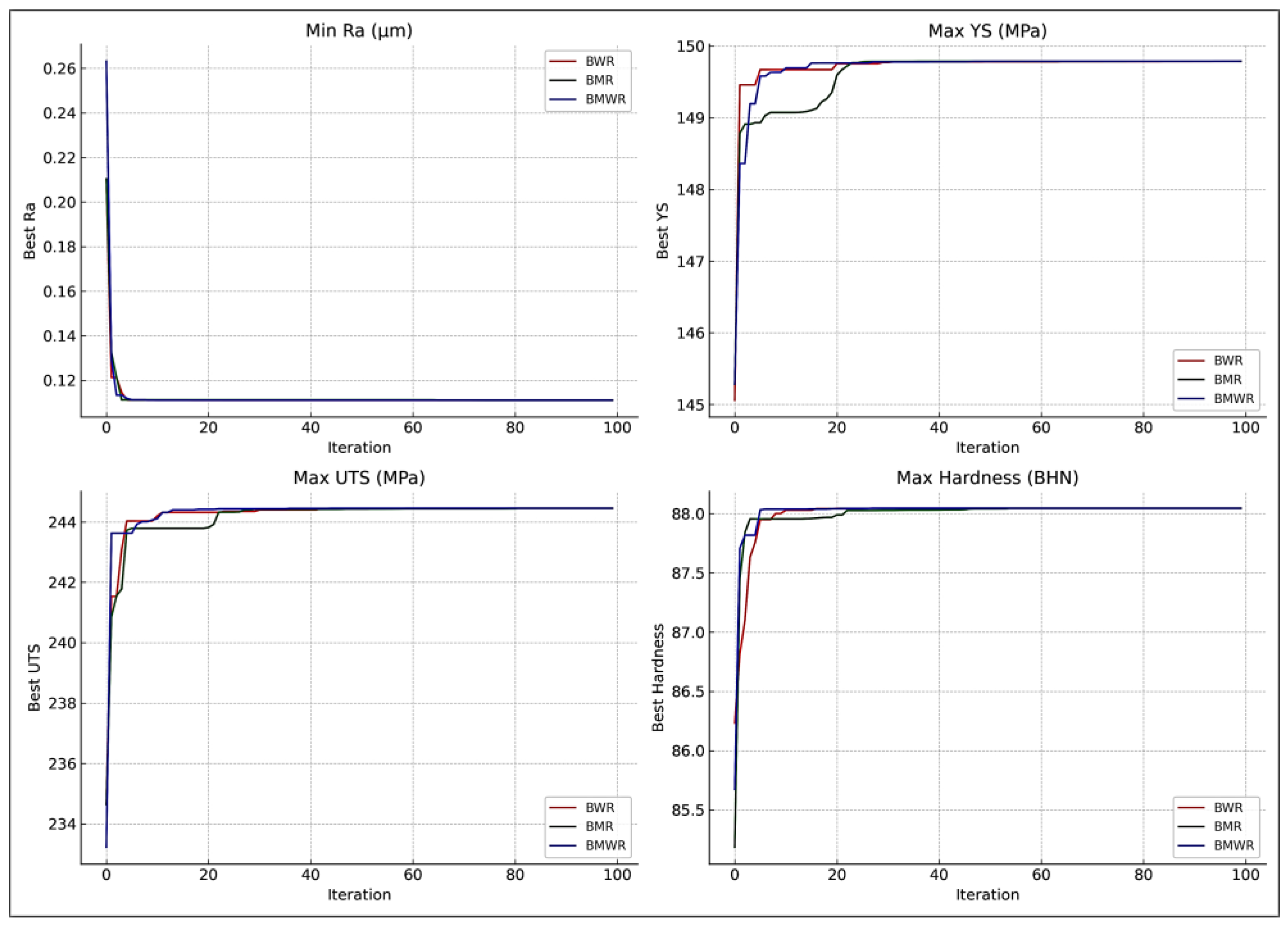
Patel et al. [11] used a genetic algorithm (GA) to solve this multi-objective problem using a priori approach (i.e., assigning different weightages to the objective functions). The population size and the iterations used in the GA were 120 and 100, respectively (i.e., the function evaluations were 120 ∗ 100 = 12,000). For the sake of comparison, the same are used in the present work using the BWR, BMR, and BMWR algorithms. At first, just to obtain the ideal optimal values of Ra, YS, UTS, and H, the three algorithms are run on the individual objective functions. The results of individual optimization are given in Table 17. The best values of the objectives obtained by the proposed algorithms are given in Table 17. It can be observed that all the three algorithms converged to the same values of respective objective functions.
Figure 14 shows the convergence graphs of the BWR, BMR, and BMWR algorithms for the four objectives Ra, YS, UTS, and H when solved for each objective function individually. All these algorithms converged to the same results.
Now, to deal with the task of simultaneously optimizing all four objectives, the proposed MO-BWR, MO-BMR, and MO-BMWR algorithms are applied each with a population size of 120 and iterations of 100 (same as those used by Patel et al. [11]). The composite front containing 94 non-repeating and Pareto-optimal non-dominated solutions (with 23 solutions from BWR, 52 from BMR, and 19 from BMWR) is formed and shown in Table 18.
As this problem contains four objectives, the best compromise solution is to be selected from the 94 Pareto-optimal solutions. BHARAT method [24] is used for normalizing the data of the objectives. In the case of the minimization of Ra, the best value is taken as 0.116302 and it is kept in the numerator and the remaining values of Ra in that column are put in the denominator to obtain the normalized data of Ra. For example, for solution 1, the normalized Ra value is 0.396482 (=0.116302/0.293334). In the case of maximization of YS, the best value is taken as 149.7124 and it is kept in the denominator and the remaining values of YS in that column are put in the numerator to obtain the normalized data of YS. A similar procedure is carried out for normalizing the data of UTS and H. The normalized data of the Ra, YS, UTS, and H are given in Table 19.
The weights of importance of the objectives can be assigned following the BHARAT method. However, to make a fair comparison with the a priori GA approach followed by Patel et al. [11], the following steps are taken.
Patel et al. [11] considered following different situations of assigning different priorities (i.e., weightages) to the objectives.
  • Case 1: Assigning equal weightages to all the objectives Ra, YS, UTS, and H, (i.e., WRa = WYS = WUTS = WH = 0.25).
  • Case 2: Assigning 70% weightage to Ra and assigning 10% weightage each to YS, UTS, and H (i.e., WRa = 0.7, WYS = WUTS = WH = 0.10).
  • Case 3: Assigning 70% weightage to YS and assigning 10% weightage each to Ra, UTS, and H (i.e., WYS = 0.7, WRa = WUTS = WH = 0.10).
  • Case 4: Assigning 70% weightage to UTS and assigning 10% weightage each to Ra, YS, and H (i.e., WUTS = 0.7, WRa = WYS = WH = 0.10).
  • Case 5: Assigning 70% weightage to H and assigning 10% weightage each to Ra, YS, and UTS (i.e., WH = 0.7, WRa = WYS = WUTS = 0.10).
For demonstration, if case 1 is considered with equal weightages of 0.25 for each of the four objectives, the composite score for solution 1 is computed as: 0.25 ∗ 0.396482 + 0.25 ∗ 0.998581 + 0.25 ∗ 1 +0.25 ∗ 0.992136 = 0.8468. Similarly, the composite scores of the 94 solutions are computed for all five cases, and the scores are listed in Table 19. It may be remembered that the solution having the highest composite score will be considered as the best compromise solution (considering all the objectives simultaneously in multi-objective optimization). The best compromise solutions are indicated in bold in Table 19 for each of the five cases.
Patel et al. [11] used GA and obtained 100 solutions and presented the compromise solutions for five cases. Now the results of the application of the proposed algorithms presented in this paper are compared with those of Patel et al. [11]. Table 20 compares the results of multi-objective optimization for the squeeze casting process for five cases. The best values of the objectives for the five cases are indicated in bold.
Even though Patel et al. [11] presented five cases, finally they recommended to use the compromise solution of case 1 with Ra = 0.1142 (µm), YS = 138.79 MPa, UTS = 228.44 MPa, and H = 85.98 BHN. However, for the same case 1 and with the same weightages of the objectives, the composite front of the present work has recommended Ra = 0.120769 (µm), YS = 140.4134 MPa, UTS = 230.0316 MPa, and H = 86.29786 BHN. The solution recommended by the present work is much better in three out of the four objectives of case 1. Similarly, it can be observed that the results of the present work are much better for three out of five cases. Thus, the composite front formed by the proposed metaphor-less and algorithm-specific control parameter-less MO-BWR, BMR, and BMWR algorithms can be understood as a viable and convenient approach for the multi-objective optimization problems.
In fact, Patel et al. [11] carried out single-objective optimization of the objectives individually (ignoring the other objectives) and then formed a combined objective function to optimize (treating that combined objective as a single objective function) using an a priori approach of GA. However, the present work considered all objectives simultaneously following an a posteriori approach. In multi-objective optimization, an a posteriori approach offers significant advantages over the a priori approach by generating the complete Pareto-optimal set before any decision-making. This allows decision-makers to visualize trade-offs between objectives, explore unexpected high-quality solutions, and avoid bias from predefined or inaccurate preferences. It is particularly valuable when preferences are uncertain or may change, as choices can be made after analyzing actual results. Additionally, it supports multi-stakeholder scenarios by enabling different decision-makers to select different solutions from the same Pareto set, ensuring flexibility, robustness, and a more informed selection process.
The Python codes for the BWR, BMR, BMWR, MO-BWR, MO-BMR, and MO-BMWR algorithms are available at: https://sites.google.com/d/1qNsqo0kHkQD9Bhi4-prZlxo5K7QuntgI/p/1OeRlPp5dhwkqfeNvLP4CtHqFhwk74DqB/edit (Accessed on 10 August 2025).
It should be emphasized that the proposed BWR, BMR, and BMWR algorithms are capable of optimizing process parameters based on the previously established empirical or regression relationships developed by the previous researchers. It should be kept in mind that the reliability of the optimization results is inherently tied to the accuracy and robustness of the regression equations employed in the optimization framework. The previous researchers reported very good statistical values corresponding to ANOVA, F-ratios, p values, and very high values of the coefficient of determination (i.e., R2) for the regression equations developed by them. Hence, the proposed algorithms are applied to those regression equations, treating them as the objective functions and the optimum values of parameters are suggested. However, the outcomes may require further validation through dedicated experiments which is not in the purview of the present work (as the aim is to prove the effective optimization of process parameters of the casting processes based on the regression equations and the simulation results reported by the researchers during the last 5 years.
The proposed algorithms (BWR, BMR, BMWR, and their multi-objective variants) differ fundamentally from machine learning (ML), deep learning (DL), and artificial neural networks (ANNs) in that they are direct metaheuristic optimizers which require only the objective functions, constraints, and variable bounds, without relying on prior datasets. They are designed to explore the solution space stochastically and provide optimal or near-optimal parameter values, often generating Pareto fronts in multi-objective scenarios. In contrast, ML/DL/ANNs are data-driven approaches that excel in regression, classification, and prediction once trained on sufficiently large and high-quality datasets, but they do not inherently perform optimization unless coupled with an optimizer. While the proposed algorithms are generally transparent, robust, and computationally efficient for parameter tuning, ML/DL/ANNs often function as black boxes requiring significant training effort, though they enable rapid predictions after training. Importantly, the two approaches can complement each other as ANNs or DL models can act as surrogate predictors of expensive simulations or experiments, while the proposed algorithms can then be used to optimize over these surrogates, resulting in a powerful hybrid strategy for complex engineering problems.
Table 21 compares the proposed BWR, BMR, and BMWR algorithms with the AI8-based optimization tools such as machine learning (ML)/deep learning (DL)/artificial neural networks (ANNs).

4. Conclusions

In this work, three novel optimization algorithms—best–worst–random (BWR), best–mean–random (BMR), and best–mean–worst–random (BMWR)—are presented and validated on a wide range of parameter optimization problems of different metal casting processes.
  • Applications to single-objective metal casting process: The BWR, BMR, and BMWR algorithms are applied to the real case studies of (i) optimization of a lost foam casting process for producing a fifth wheel coupling shell from EN-GJS-400-18 ductile iron, (ii) optimization of process parameters of die casting of A360 Al-alloy, and (iii) optimization of wear rate of an AA7178 alloy reinforced with nano-SiC particles produced using a stir-casting process. Comparisons of results are made with RSM and ProCAST 2021 simulations in case study (i), RSM and CAE simulation software in case study (ii), and the metaheuristics such as ABC, Rao-1, and PSO algorithms in case study (iii). The three algorithms achieve better results compared to the simulation software and the metaheuristics. The proposed algorithms showed faster convergence and superior solution quality with fewer function evaluations, highlighting their computational efficiency. For single-objective optimization, BWR, BMR, and BMWR provided the same results for the case studies considered. In general, these three algorithms provide almost the same results with minor variations in the case of single-objective optimization problems. But it is not so in the case of multi-objective optimization problems. Their performances may give different Pareto fronts (and some Pareto front solutions may match), and hence a composite front concept that takes into account all non-duplicated and unique non-dominated solutions is suggested in this paper for the multi-objective optimization of metal casting processes.
  • Applications to multi-objective metal casting processes: The multi-objective variants (MO-BWR, MO-BMR, and MO-BMWR) are tested on (iv) two-objectives optimization of a low-pressure casting process using a sand mold for producing A356 engine block and (v) four-objective optimization of a squeeze casting process for LM20 material. These are compared with established methods such as NSGA-II and FEA simulation in case study (iv), and the a priori approach of GA in case study (v). The results show that competitive performance is achievable without added complexity, making the proposed algorithms transparent, interpretable, robust, and versatile for optimizing metal casting processes.
  • Decision-making integration: This study employs the BHARAT method—a structured MADM approach—to select the most suitable compromise solutions from Pareto-optimal sets, especially when visual interpretation is impractical in multi-objective problems. This leads to better decision-making for choosing the optimal process parameters in the case of multi-objective optimization problems.
  • Broader applicability: The findings suggest that these algorithms are well suited for a wide range of real-world manufacturing challenges across high-dimensional settings and constrained/unconstrained problems alike. Applications include additive manufacturing process optimization, toolpath planning, welding parameter tuning, multi-axis machining, and thermal processing, with further potential through coupling with ML, DL, and ANN models for data-driven workflows. The versatility, scalability, and robustness of the BWR, BMR, and BMWR algorithms make them promising tools for the future of intelligent manufacturing optimization.

Author Contributions

Conceptualization, R.V.R.; methodology, R.V.R.; validation, R.V.R.; formal analysis and writing—original draft preparation, R.V.R.; writing—review and editing, J.P.D. and R.V.R. All authors have read and agreed to the published version of the manuscript.

Funding

This research received no external funding to meet the APC.

Data Availability Statement

All original contributions from this study are contained within the article; further inquiries may be addressed to the corresponding author.

Acknowledgments

Support from the Anusandhan National Research Foundation of the Government of India (MTR/2023/000071) is gratefully acknowledged by the first author. We thank M. V. Harishankar for contributions to the ZDT functions. Certain figures and interpretations were prepared with the assistance of ChatGPT-4o. The authors have reviewed and edited the output and take full responsibility for the content of this publication.

Conflicts of Interest

The authors declare no conflicts of interest.

Appendix A

The results of MO-BWR, MO-BMR, and NSGA-III are taken from recent work of Rao and Davim [22]. The convergence graphs for these algorithms are available in [22]. Hence, in this paper convergence graphs of the newly proposed MO-BMWR algorithm are produced and are shown in Figure A1.
Furthermore, for comparison purposes the results of different algorithms presented by Ravichandran et al. [24] are also considered. These algorithms included multi-objective adaptive guided differential evaluation (MOAGDE), improved multi-objective particle swarm optimization (MOIPSO), multi-objective gradient-based optimizer (MOGBO), NSGA-II (non-dominated sorting genetic algorithm II), and multi-objective resistance-capacitance optimization algorithm (MOR-COA). Each algorithm is executed 30 times independently, with 40,000 function evaluations, to ensure a fair comparison.
The comparison of results of these eight algorithms with reference to the performance metrics of mean spacing, mean hypervolume, mean generational distance (GD), mean inverted generational distance (IGD), and mean spread are shown in Table A1, Table A2, Table A3, Table A4 and Table A5 of Appendix A. The numbers shown in parentheses in Table A1, Table A2, Table A3, Table A4 and Table A5 show the standard deviation values. Standard deviation values are presented only for the BWR, BMR, BMWR, and NSGA-III algorithms, while those for other algorithms are omitted here to avoid similarity issues as their results are already reported in Ravichandran et al. [24].
It may be noted that spacing indicates the uniformity of spacing between consecutive solutions in the obtained Pareto front. Lower spacing indicates better distribution uniformity. Hypervolume measures the region in the objective space that is dominated by the obtained Pareto front and bounded by a reference point. A higher hypervolume value signifies better convergence and diversity. Generational distance (GD) calculates the average Euclidean distance from each obtained solution to the closest point on the true Pareto front, with lower values indicating better convergence. Inverted generational distance (IGD) computes the average distance from each point on the true Pareto front to its nearest counterpart in the obtained solution set; lower IGD values indicate good convergence along with diversity. Spreading evaluates how uniformly and extensively the non-dominated (Pareto-optimal) solutions are distributed across the Pareto front, with lower values being preferable.
From the results presented in Table A1, Table A2, Table A3, Table A4 and Table A5 of Appendix A, it can be observed that the top three performers (in spacing) are MO-BMR, MO-BWR, and MO-BMWR. These three consistently produce evenly distributed Pareto fronts, which is critical for maintaining diversity and decision flexibility. NSGA-III is only competitive in ZDT6. Classical and other metaheuristics struggle with spacing.
Figure A1. Convergence behavior of MO-BMWR algorithm for ZDT functions.
Metals 15 01057 g0a1
The top three performers (in hypervolume) are MO-BMR, MO-BMWR, and MO-BWR. These algorithms consistently outperform all traditional and many modern algorithms across every ZDT problem. NSGA-III is competitive, but not better than these algorithms. MO-BMWR and MO-BMR are the most balanced in convergence, diversity, and front coverage.
The top three algorithms (in GD) are MOR-COA, NSGA-III, and MOIPSO. Compared to MO-BWR and MO-BMWR, the MO-BMR performs best overall. The best overall performers (in IGD) are MO-BMR, MO-BMWR, and MO-BWR. These algorithms significantly outperform classical methods (NSGA-II, NSGA-III, MOIPSO, etc.) in terms of both accuracy and diversity. MO-BMR is particularly consistent and accurate across all problems.
The top three algorithms (in spread) are NSGA-III, MOAGDE, and MOR-COA. NSGA-III consistently provides the best diversity (lowest spread) across all problems. MO-BWR, MO-BMR, and MO-BMWR offer reasonable performance, but need improvement in maintaining spread. NSGA-II, MOIPSO, and MOGBO mostly show higher spread values, indicating poorer diversity.
Table A1. Comparison of algorithms with reference to mean spacing.
ProblemNSGA-II [24]MOIPSO [24]MOAGDE [24]MOGBO [24]MORCOA [24]MO-BWRMO-BMRMO-BMWRNSGA-III
ZDT11.8507 × 10−21.3665 × 10−27.9902 × 10−31.6956 × 10−22.2389 × 10−20.0005928
(2.4024 × 10⁻⁵)
0.000633
(1.9272 × 10⁻⁵)
6.0783 × 10−04 [7.9093 × 10⁻⁵]0.010218
(4.3086 × 10⁻⁴)
ZDT21.5718 × 10−21.3397 × 10−29.5609 × 10−31.6123 × 10−28.6954 × 10−3 0.000821
(5.6432 × 10⁻⁴)
0.001060
(7.2644 × 10⁻⁴)
1.5277 × 10⁻³ [8.5514 × 10⁻⁵]0.004172
(2.9634 × 10⁻⁵)
ZDT31.8403 × 10−21.5737 × 10−23.2391 × 10−2 1.7805 × 10−22.3700 × 10−20.0012825
(3.4899 × 10⁻⁴)
0.0008835
(3.3653 × 10⁻⁴)
9.8901 × 10⁻⁴ [3.4633 × 10⁻⁴]0.007505
(1.7482 × 10⁻⁴)
ZDT41.8022 × 10−22.1423 × 10−28.0906 × 10−33.5745 × 10−21.8508 × 10−20.001852
(8.3442 × 10⁻⁵)
0.001803
(1.1073 × 10⁻⁴)
1.8412 × 10⁻³ [8.8294 × 10⁻⁵]0.010484
(4.8832 × 10⁻⁴)
ZDT61.3490 × 10−21.7261 × 10−17.0428 × 10−36.9157 × 10−24.3206 × 10−30.054858
(7.5815 × 10⁻²)
0.068319
(7.3691 × 10⁻²)
3.1609 × 10⁻² [6.8207 × 10⁻²]0.002476
(1.0359 × 10⁻⁴)
Table A2. Comparison of algorithms with reference to mean hypervolume.
ProblemNSGA-II [24]MOIPSO [24]MOAGDE [24]MOGBO [24]MORCOA [24]MO-BWRMO-BMRMO-BMWRNSGA-III
ZDT17.1001 × 10−17.1584 × 10−17.1508 × 10−17.1202 × 10−17.1367 × 10−10.875832
(2.7768 × 10⁻⁴)
0.876091
(1.7750 × 10⁻⁵)
8.7585 × 10⁻¹ [2.5627 × 10⁻⁴]0.871460
(5.9923 × 10⁻⁵)
ZDT24.3822 × 10−14.4061 × 10−14.3711 × 10−14.3831 × 10−14.4099 × 10−10.527392
(7.5723 × 10⁻³)
0.539351
(1.6764 × 10⁻³)
5.4111 × 10⁻¹ [1.0968 × 10⁻³]0.538386
(2.4044 × 10⁻⁵)
ZDT35.9737 × 10−15.9804 × 10−16.1872 × 10−15.9761 × 10−15.9735 × 10−10.72128
(6.9315 × 10⁻³)
0.72463
(5.4288 × 10⁻³)
7.2442 × 10⁻¹ [5.3662 × 10⁻³]0.724230
(7.6240 × 10⁻⁵)
ZDT47.1339 × 10−10.0000e+07.0461 × 10−11.4846 × 10−17.1533 × 10−10.872858
(2.9916 × 10⁻⁴)
0.872257
(6.4334 × 10⁻⁴)
8.7258 × 10⁻¹ [6.0676 × 10⁻⁴]0.867990
(5.2656 × 10⁻³)
ZDT63.8417 × 10−13.8400 × 10−13.8198 × 10−13.8406 × 10−13.8595 × 10−10.615821
(1.7178 × 10⁻⁵)
0.615820
(1.8577 × 10⁻⁵)
6.1574 × 10⁻¹ [1.6094 × 10⁻⁵]0.607590
(3.2857 × 10⁻⁴)
Table A3. Comparison of algorithms with reference to mean GD.
ProblemNSGA-II [24]MOIPSO [24]MOAGDE [24]MOGBO [24]MORCOA [24]MO-BWRMO-BMRMO-BMWRNSGA-III
ZDT17.2045 × 10−45.5523 × 10−52.3922 × 10−41.6882 × 10−47.0812 × 10−60.005128
(1.1805 × 10⁻⁴)
0.005051
(7.3743 × 10⁻⁵)
5.1523 × 10⁻³ [2.2083 × 10⁻⁴]0.003548
(5.0038 × 10⁻⁵)
ZDT24.9576 × 10−45.9375 × 10−68.3658 × 10−42.2611 × 10−46.4197 × 10−60.004021
(5.1599 × 10⁻⁴)
0.004121
(6.2991 × 10⁻⁴)
4.1159 × 10⁻³ [3.0825 × 10⁻⁴]0.003609
(1.5771 × 10⁻⁵)
ZDT31.6936 × 10−45.1251 × 10−59.2672 × 10−48.6095 × 10−57.6050 × 10−50.003869
(3.2657 × 10⁻⁴)
0.003633
(2.5603 × 10⁻⁴)
3.6800 × 10⁻³ [3.6984 × 10⁻⁴]0.002818
(5.8555 × 10⁻⁵)
ZDT41.1637 × 10−46.4948 × 10−11.4447 × 10−32.0847 × 10−17.3824 × 10−50.005478
(1.5433 × 10⁻⁴)
0.005676
(2.9654 × 10⁻⁴)
5.6024 × 10⁻³ [2.6104 × 10⁻⁴]0.004254
(6.5069 × 10⁻⁴)
ZDT61.3663 × 10−51.1629 × 10−17.2840 × 10−49.0456 × 10−34.9198 × 10−60.006370
(4.1160 × 10⁻³)
0.007295
(4.1911 × 10⁻³)
4.8786 × 10⁻³ [2.3941 × 10⁻³]0.004303
(1.4614 × 10⁻⁴)
Table A4. Comparison of algorithms with reference to mean IGD.
ProblemNSGA-II [24]MOIPSO [24]MOAGDE [24]MOGBO [24]MORCOA [24]MO-BWRMO-BMRMO-BMWRNSGA-III
ZDT11.2703 × 10−28.2757 × 10−37.8680 × 10−31.0942 × 10−29.8560 × 10−30.000549
(1.6931 × 10⁻⁴)
0.000435
(3.2228 × 10⁻⁵)
5.3919 × 10⁻⁴ [1.6076 × 10⁻⁴], 0.003543
(6.8238 × 10⁻⁵)
ZDT21.0230 × 10−28.4165 × 10−38.9290 × 10−39.8612 × 10−37.6915 × 10−30.018096
(9.1079 × 10⁻²)
0.002203
(8.3148 × 10⁻³)
1.3404 × 10⁻³ [4.2971 × 10⁻⁴]0.003438
(1.6013 × 10⁻⁵)
ZDT31.0944 × 10−29.9319 × 10−32.8845 × 10−21.1069 × 10−21.2028 × 10−20.003187
(2.8226 × 10⁻³)
0.001671
(2.2589 × 10⁻³)
1.7209 × 10⁻³ [2.1574 × 10⁻³]0.003709
(1.0524 × 10⁻⁴)
ZDT49.8920 × 10−34.1352e+01.3027 × 10−21.1744e+07.8954 × 10−30.002180
(1.5306 × 10⁻⁴)
0.002498
(3.6697 × 10⁻⁴)
2.3071 × 10⁻³ [3.4921 × 10⁻⁴]0.005634
(1.3859 × 10⁻³)
ZDT67.7923 × 10−37.9355 × 10−37.7894 × 10−37.9693 × 10−36.0637 × 10−30.000418
(2.8515 × 10⁻⁵)
0.000424
(2.8036 × 10⁻⁵)
4.6332 × 10⁻⁴ [3.2756 × 10⁻⁵]0.004245
(1.3982 × 10⁻⁴)
Table A5. Comparison of algorithms with reference to mean spread.
ProblemNSGA-II [24]MOIPSO [24]MOAGDE [24]MOGBO [24]MORCOA [24]MO-BWRMO-BMRMO-BMWRNSGA-III
ZDT14.3487 × 10−13.1745 × 10−12.5930 × 10−14.9742 × 10−12.9873 × 10−13.1361 × 10⁻¹ [1.1120 × 10⁻²]3.2806 × 10⁻¹ [1.0249 × 10⁻²]3.2199 × 10⁻¹ [3.8097 × 10⁻²]1.0218 × 10⁻² [4.3086 × 10⁻⁴]
ZDT24.4451 × 10−13.2170 × 10−11.6461 × 10−14.5021 × 10−11.4780 × 10−14.0886 × 10⁻¹ [1.9311 × 10⁻¹]3.7987 × 10⁻¹ [2.2124 × 10⁻¹]3.1730 × 10⁻¹ [1.6494 × 10⁻²]4.1718 × 10⁻³ [2.9634 × 10⁻⁵]
ZDT34.3451 × 10−13.4276 × 10−15.8171 × 10−14.0807 × 10−15.9475 × 10−11.1641 × 10⁻¹ [9.8612 × 10⁻²]1.0645 × 10⁻¹ [1.2725 × 10⁻¹]1.0169 × 10⁻¹ [1.0970 × 10⁻¹]7.5058 × 10⁻³ [1.7482 × 10⁻⁴]
ZDT46.0984 × 10−18.1658 × 10−12.5680 × 10−18.1966 × 10−12.9792 × 10−12.8269 × 10⁻¹ [1.3513 × 10⁻²]2.7832 × 10⁻¹ [1.4771 × 10⁻²]2.7892 × 10⁻¹ [1.3435 × 10⁻²]1.0484 × 10⁻² [4.8832 × 10⁻⁴]
ZDT65.3100 × 10−11.1330 × 1001.5160 × 10−17.1663 × 10−11.0774 × 10−17.4914 × 10⁻¹ [4.6623 × 10⁻¹]8.7928 × 10⁻¹ [4.7150 × 10⁻¹]5.5934 × 10⁻¹ [3.8586 × 10⁻¹]2.4764 × 10⁻³ [1.0359 × 10⁻⁴]

References

  1. Xu, Z.; Chen, T.; Li, B.; Wang, C.; Yang, S.; Chen, Y.; Guo, Z.; Zhang, W.; Guan, R. Optimization of process parameters and microstructure prediction of A360 Al-alloy during die casting. Int. J. Metalcast. 2025, 1–13. [Google Scholar] [CrossRef]
  2. Li, J.; Wang, D.; Xu, Q. Research on the squeeze casting process of large wheel hub based on FEM and RSM. Int. J. Adv. Manuf. Technol. 2023, 127, 1445–1458. [Google Scholar] [CrossRef]
  3. Triller, J.; Lopez, M.L.; Nossek, M.; Frenzel, M.A. Multidisciplinary optimization of automotive mega-castings using RSM enhanced by machine learning. Sci. Rep. 2023, 13, 4532. [Google Scholar] [CrossRef]
  4. Deng, W.; Song, Z.; Lei, J.; Luo, K.; Zhang, Y.; Yu, M. Multi-objective optimization of A356 engine block casting process parameters based on response surface method and NSGA II genetic algorithm. Int. J. Metalcast. 2025, 1–19. [Google Scholar] [CrossRef]
  5. Bharat, N.; Akhil, G.; Bose, P.S.C. Metaheuristic approach to enhance wear characteristics of novel AA7178/nSiC metal matrix composites. J. Mater. Eng. Perform. 2024, 33, 12638–12655. [Google Scholar] [CrossRef]
  6. He, B.; Lei, Y.; Jiang, M.; Wang, F. Optimal design of the gating and riser system for complex casting using an evolutionary algorithm. Materials 2022, 15, 7490. [Google Scholar] [CrossRef]
  7. Deshmukh, S.; Ingle, A.; Thakur, D. Optimization of stir casting process parameters in the fabrication of aluminium based metal matrix composites. Mater. Today Proc. 2023, 82, 485–490. [Google Scholar] [CrossRef]
  8. Kavitha, M.; Raja, V. Optimization of Insert Roughness and Pouring Conditions to Maximize Bond Strength of (Cp)Al-SS304 Bimetallic Castings Using RSM-GA Coupled Technique. Mater. Today Commun. 2024, 39, 108754. [Google Scholar] [CrossRef]
  9. Patel, D.S.; Nayak, R.K. Design and Development of Copper Slag Mold for A-356 Alloy Casting. Trans. Indian Inst. Met. 2025, 78, 48. [Google Scholar] [CrossRef]
  10. Panicker, P.G.; Kuriakose, S. Parameter Optimisation of Squeeze Casting Process Using LM 20 Alloy: Numeral Analysis by Neural Network and Modified Coefficient-Based Deer Hunting Optimization. Aust. J. Mech. Eng. 2020, 21, 351–367. [Google Scholar] [CrossRef]
  11. Patel, G.C.M.; Krishna, P.; Parappagoudar, M.B. Modelling and Multi-Objective Optimisation of Squeeze Casting Process Using Regression Analysis and Genetic Algorithm. Aust. J. Mech. Eng. 2015, 14, 182–198. [Google Scholar] [CrossRef]
  12. Li, H.; Ji, H.; Chen, B.; Huang, X.; Xing, M.; Cui, G.; Qiu, C. Optimization of Defects in the Lost Foam Casting Process for Fifth Wheel Coupling Shell. Int. J. Met. 2025, 1–17. [Google Scholar] [CrossRef]
  13. Simon, D. Evolutionary Optimization Algorithms: Biologically-Inspired and Population-Based Approaches to Computer Intelligence; John Wiley & Sons: Hoboken, NJ, USA, 2013. [Google Scholar]
  14. Salgotra, R.; Sharma, P.; Raju, S.; Gandomi, A.H. A contemporary systematic review on meta-heuristic optimization algorithms with their MATLAB and Python code reference. Arch. Comput. Methods Eng. 2024, 31, 1749–1822, Erratum in Arch. Comput. Methods Eng. 2024, 31, 1749–1822. [Google Scholar] [CrossRef]
  15. Rajwar, K.; Deep, K.; Das, S. An exhaustive review of the metaheuristic algorithms for search and optimization: Taxonomy, applications, and open challenges. Artif. Intell. Rev. 2023, 56, 13187–13257. [Google Scholar] [CrossRef]
  16. Benaissa, B.; Kobayashi, M.; Ali, M.A.; Khatir, T.; Elmeliani, M.E.A.E. Metaheuristic optimization algorithms: An overview. HCMCOUJS-Adv. Comput. Struct. 2024, 14, 34–62. [Google Scholar] [CrossRef]
  17. Rao, R.V. Rao algorithms: Three metaphor-less simple algorithms for solving optimization problems. Int. J. Ind. Eng. Comput. 2020, 11, 107–130. [Google Scholar]
  18. Sörensen, K. Metaheuristics—The metaphor exposed. Int. Trans. Oper. Res. 2015, 22, 3–18. [Google Scholar] [CrossRef]
  19. Aranha, C.L.C.; Villalón, F.; Dorigo, M.; Ruiz, R.; Sevaux, M.; Sörensen, K.; Stützle, T. Metaphor-based metaheuristics, a call for action: The elephant in the room. Swarm Intell. 2021, 16, 1–6. [Google Scholar] [CrossRef]
  20. Velasco, L.; Guerrero, H.; Hospitaler, A. A literature review and critical analysis of metaheuristics recently developed. Arch. Comput. Methods Eng. 2023, 31, 125–146. [Google Scholar] [CrossRef]
  21. Sarhani, M.; Voß, S.; Jovanovic, R. Initialization of metaheuristics: Comprehensive review, critical analysis, and research directions. Int. Trans. Oper. Res. 2022, 30, 3361–3397. [Google Scholar] [CrossRef]
  22. Rao, R.V.; Davim, J.P. Single, multi-, and many-objective optimization of manufacturing processes using two novel and efficient algorithms with integrated decision-making. J. Manuf. Mater. Process. 2025, 9, 249. [Google Scholar] [CrossRef]
  23. Rao, R.V. BHARAT: A simple and effective multi-criteria decision-making method that does not need fuzzy logic, Part-1: Multi-attribute decision-making applications in the industrial environment. Int. J. Ind. Eng. Comput. 2024, 15, 13–40. [Google Scholar] [CrossRef]
  24. Ravichandran, S.; Manoharan, P.; Sinha, D.K.; Jangir, P.; Abualigah, L.; Alghamdi, T.A.H. Multi-objective resistance–capacitance optimization algorithm: An effective multi-objective algorithm for engineering design problems. Heliyon 2024, 10, e35921. [Google Scholar] [CrossRef] [PubMed]
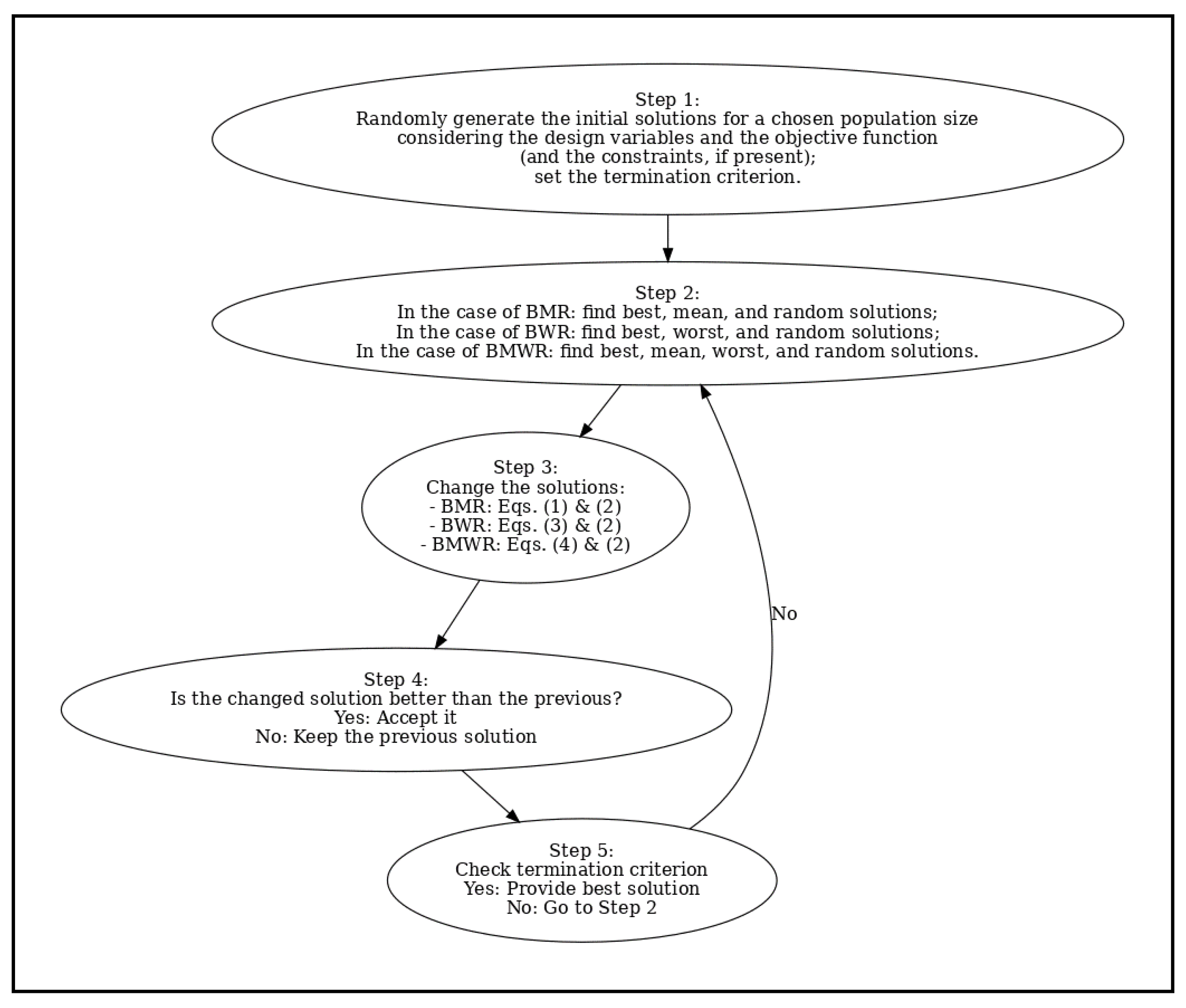
Figure 1. Flowchart of BWR, BMR, and BMWR algorithms.
Metals 15 01057 g001
Figure 2. Pseudocodes of BWR, BMR, and BMWR algorithms.
Metals 15 01057 g002
Figure 3. Convergence behavior of BWR, BMR, and BMWR algorithms.
Metals 15 01057 g003
Figure 4. Convergence behavior of the algorithms for lost foam casting process.
Metals 15 01057 g004
Figure 5. Surface plots showing the effects of A, B, and C on porosity P.
Metals 15 01057 g005
Figure 6. Convergence behavior of the algorithms for the die casting process.
Metals 15 01057 g006
Figure 7. Surface plots showing the effects of TC, TM, and V on volumetric porosity P.
Metals 15 01057 g007
Figure 8. Convergence behavior of the algorithms for wear rate of a stir-cast MMC.
Metals 15 01057 g008
Figure 9. Surface plots showing the effects of A, B, C, and D on the wear rate.
Metals 15 01057 g009
Figure 10. Convergence behavior of the algorithms for minimum solidification time.
Metals 15 01057 g010
Figure 11. Convergence behavior of the algorithms for minimum shrinkage volume.
Metals 15 01057 g011
Figure 12. Pareto composite front for the low-pressure casting process.
Metals 15 01057 g012
Figure 13. Surface plots showing the effect of the process parameters on Y1 and Y2.
Metals 15 01057 g013
Figure 14. Convergence behavior of the proposed algorithms on Ra, YS, UTS, and H.
Metals 15 01057 g014
Table 1. Initially generated random population.
Solutionx1x2f(x)c1(x)p1c2(x)p2c3(x)p3M(x)
10.374540.9507141.0441380.3252540.10579−0.174540−0.6507101.149928 (worst)
20.7319940.5986580.8942070.3306520.109331−0.531990−0.2986601.003538
30.1560190.1559950.048676−0.6879900.0439810.0019340.1440050.0207380.071348 (best)
40.0580840.8661760.753635−0.0757400.1419160.02014−0.5661800.773775
50.6011150.7080730.8627060.3091880.095597−0.401120−0.4080700.958303
Table 2. Modified variable values, constraint evaluations, penalty terms, and objective function results obtained using the BWR algorithm.
Solutionx1x2f(x)c1(x)p1c2(x)p2c3(x)p3M(x)
10.2675450.7748630.6719920.0424070.001798−0.0675450−0.4748600.673791
20.7336050.3911780.6911960.1247830.015571−0.5336050−0.09117800.706767
30.18380600.033788−0.81619400.0161940.0002620.30.090.124047
400.5482880.30062−0.45171200.20.04−0.24828800.34062
50.5574110.5491290.612250.106540.011351−0.3574110−0.24912900.6236
Table 3. Updated variable values, evaluated constraints, corresponding penalties, and objective function results obtained using the BWR algorithm.
Solutionx1x2f(x)c1(x)p1c2(x)p2c3(x)p3M(x)
10.2675450.7748630.6719920.0424070.001798−0.0675450−0.4748600.673791
20.7336050.3911780.6911960.1247830.015571−0.5336050−0.09117800.706767 (worst)
30.1560190.1559950.048676−0.6879900.0439810.0019340.1440050.0207380.071348 (best)
400.5482880.30062−0.45171200.20.04−0.24828800.34062
50.5574110.5491290.612250.106540.011351−0.3574110−0.24912900.6236
Table 4. Final (1000th iteration) values of the variables, constraints, penalties, and objective function results obtained using the BWR algorithm.
Solutionx1x2f(x)c1(x)p1c2(x)p2c3(x)p3M(x)
10.20.30.13−0.5000000.13
20.20.30.13−0.5000000.13
30.20.30.13−0.5000000.13
40.20.30.13−0.5000000.13
50.20.30.13−0.5000000.13
Table 5. Modified variable values, constraint evaluations, penalty terms, and objective function results obtained using the BMR algorithm.
Solutionx1x2f(x)c1(x)p1c2(x)p2c3(x)p3M(x)
10.3680480.5666560.456558−0.0652960−0.1680480−0.26665600.456558
20.5082890.2778330.335549−0.2138770−0.30828900.221670.0004910.336041
3000−100.20.040.30.090.13
40.0124180.7661910.587202−0.22139200.1875820.035187−0.46619100.622389
50.468040.29020.303278−0.241760−0.2680400.00980.0000960.303374
Table 6. Updated variable values, evaluated constraints, corresponding penalties, and objective function results obtained using the BMR algorithm.
Solutionx1x2f(x)c1(x)p1c2(x)p2c3(x)p3M(x)
10.3680480.5666560.456558−0.0652960−0.1680480−0.26665600.456558
20.5082890.2778330.335549−0.2138770−0.30828900.221670.0004910.336041
30.1560190.1559950.048676−0.6879900.0439810.0019340.1440050.0207380.071348
40.0124180.7661910.587202−0.22139200.1875820.035187−0.46619100.622389
50.468040.29020.303278−0.241760−0.2680400.00980.0000960.303374
Table 7. Modified variable values, constraint evaluations, penalty terms, and objective function results obtained using the BMWR algorithm.
Solutionx1x2f(x)c1(x)p1c2(x)p2c3(x)p3M(x)
10.2022910.8169130.7082690.0192050.000369−0.0022910−0.51691300.708638
20.7769580.4016080.7649530.1785660.031886−0.5769580−0.10160800.796838
30.25333400.064178−0.7466660−0.05333400.30.090.154178
400.4483030.200976−0.55169700.20.04−0.14830300.240976
50.55544906080880.6782940.1635360.026744−0.3554490−0.30808800.705038
Table 8. Updated values of the variables, evaluated constraints, associated penalties, and the objective function results obtained using the BMWR algorithm.
Solutionx1x2f(x)c1(x)p1c2(x)p2c3(x)p3M(x)
10.2022910.8169130.7082690.0192050.000369−0.0022910−0.51691300.708638
20.7769580.4016080.7649530.1785660.031886−0.5769580−0.10160800.796838
30.1560190.1559950.048676−0.6879900.0439810.0019340.1440050.0207380.071348
400.4483030.200976−0.55169700.20.04−0.14830300.240976
50.55544906080880.6782940.1635360.026744−0.3554490−0.30808800.705038
Table 9. Salient features of the BWR, BMR, and BMWR algorithms.
FeatureBWRBMRBMWR
Search mechanism typeHybrid arithmetic with best–worst–random guidanceHybrid arithmetic with best–mean–random guidanceHybrid arithmetic combining best–mean–worst–random
Novel equation logicCombines (best–F × random) and (worst–random) differences; fallback to uniform samplingCombines (best–F × mean) and (best–random); fallback to uniform samplingCombines (best–F × mean) and (worst–random); fallback to uniform sampling
Handling of random influenceDirect—random solution explicitly part of updateSame as BWRSame as BWR and BMR
Fallback samplingYes: if r4 ≤ 0.5, fallback to uniform random within boundsSame as BWRSame as BWR
Diversity mechanismVery strong, due to combination of best, worst, and random solutionsStrong, but more conservative due to mean guidanceVery strong, integrates best, mean, worst, and random
Exploration–exploitation balanceHighly exploratory, still exploits bestMore exploitative, smoother convergence via mean-based pullBalanced—exploration from worst/random, exploitation from best/mean
Design simplicitySlightly complex (two difference terms + fallback), but parameter-free and metaphor-freeSimilarly to BWR and still parameter-freeSlightly more complex (all four references), but parameter-free
Robustness to local optimaStrong—fallback randomness + worst guidance help escapeGood, but conservative due to mean-based biasStrongest—mixed forces reduce trapping in local optima
Risk of premature convergenceLow (due to worst + random)Low–moderate (mean pulls population together)Low (conflicting forces maintain diversity)
Parameter dependenceNone beyond population size and iterationsNone beyond population size and iterationsNone beyond population size and iterations
Convergence speedSlower—broad exploration before exploitationFaster—mean accelerates convergenceIntermediate—not as fast as BMR, but more diverse
Constraint handling compatibilityWorks well with penalty methods, strong exploration helps recover feasibilityMay converge prematurely in tight feasible spacesMore robust than both, balances feasibility search and convergence
Multi-objective performanceProduces well-spread Pareto sets due to strong diversityGenerates smoother but sometimes narrower Pareto setsBest compromise—well-distributed and convergent Pareto fronts
Scalability with dimensionalityMay lose efficiency in very high dimensions (overexplores)Stable, but risks local trapping as dimensions growBetter scalability—multiple guiding forces adapt well
Computational cost per iterationLight—simple difference calculationsSame as BWRSlightly higher (two guiding forces), but still lighter than GA/PSO/DE
Table 10. Procedural steps of the MO-BWR, MO-BMR, and MO-BMWR algorithms.
Step No.Step TitleDescription
1StartInitiate the algorithm.
2Initialize populationGenerate the initial set of solutions within defined variable bounds.
3Elite seedingIntroduce high-quality or historically good solutions into the initial population.
4Fast non-dominated sortingRank solutions based on Pareto dominance and compute crowding distance.
5Constraint repairTry to rectify any constraint violations in the solutions as the primary strategy.
6Penalty applicationImpose penalties on the objective functions if constraint violations persist (fallback strategy).
7Objective function evaluationAssess all objective functions for every solution in the population.
8Edge boostingPromote exploration in regions close to the extreme ends of the Pareto front.
9Local explorationImprove elite or high-potential solutions by conducting a search in their local neighborhood.
10Population update (BWR/BMR/BMWR)Create new candidate solutions using the specific update mechanism of BWR, BMR, or BMWR.
11Check termination criterionCheck if the stopping condition (e.g., maximum iterations or evaluations) has been reached.
12If not terminated, repeat (go to step 5)If termination condition is not met, return to Step 5 and continue the process.
13If terminated, output solutionsTerminate the algorithm and present the final set of non-dominated Pareto-optimal solutions.
Table 11. Comparison of optimal porosity obtained in a lost foam casting process for producing a fifth wheel coupling shell from EN-GJS-400-18 ductile iron.
MethodOptimal Porosity
(%)
Process Input Parameters
Pouring Temperature A (°C)Pouring Speed B (kg/s)Ferro-Static Head Pressure C (Pa)
Simulation by RSM and ProCAST 2021 [12]0.792013866.42109751
BWR0.763513506.5110000
BMR0.763513506.5110000
BMWR0.763513506.5110000
Table 12. Comparison of optimal volumetric porosity obtained in the die casting process for producing A360 Al-alloy cover plate.
MethodOptimal Volumetric Porosity (cm3) Process Input Parameters
Casting Temperature TC (°C)Mold Preheating Temperature TM (°C)Fast Injection Speed V (m/s)
Simulation by RSM and CAE software [1]0.9203 (corrected value)6302202.5
BWR0.89956302203.5
BMR0.89956302203.5
BMWR0.89956302203.5
Table 13. Comparison of optimal wear rate obtained in stir casting by different algorithms.
AlgorithmOptimal Wear Rate ((mm3/m) ∗ 10−3)Optimum Values of Input Variables
A (m/s)B (m)C (N)D (%)
ABC [5]1.7093Not givenNot givenNot givenNot given
Rao-1 [5]1.708845009.813
PSO [5]2.1809Not givenNot givenNot givenNot given
BWR1.708845009.813
BMR1.708845009.813
BMWR1.708845009.813
Table 14. Performance metrics for the three algorithms for the low-pressure casting process.
AlgorithmGDIGDSpacingSpreadHypervolume
MO-BWR00.1627570.2677710.8360690.516014
MO-BMR00.0652840.0215350.8450450.623620
MO-BMWR00.0327640.0457400.5068410.731088
Composite000.0427010.8118910.762125
Table 15. Forty unique non-dominated optimal solutions from the composite front (MO-BWR + MO-BMR + MO-BMWR) for the low-pressure casting process.
S.No.A (°C)B (°C)C (s)D (kPa)Y1 (s)Y2 (cm3)AlgorithmNormalized Y1Normalized Y2Score
1680201050734.713575.14654MO-BWR0.9897480.9928430.991296
2685.484625.4845911.3711554.11345757.342674.92711MO-BWR0.9601750.9957510.977963
3708.884436.0202315.9039971.66332827.346674.60873MO-BWR0.87893210.939466
4684.972724.9727211.2431853.72954755.304474.94447MO-BWR0.9627660.995520.979143
5685.449125.4490911.3622754.08682757.201774.9283MO-BWR0.9603530.9957350.978044
6686.13826.1380111.534554.60351759.922474.9059MO-BWR0.9569150.9960330.976474
7682.04222010.5105451.53162742.95575.04257MO-BWR0.9787690.9942190.986494
8688.06628.0660412.0165156.04953767.390574.84942MO-BWR0.9476030.9967840.972193
9688.004728.0047212.0011856.00354767.156374.85108MO-BWR0.9478920.9967620.972327
10694.056529.8546813.5141360.54238787.931274.69669MO-BWR0.9228990.9988220.960861
11682.25372010.5634351.69028743.790175.03229MO-BWR0.977670.9943550.986012
12691.772731.7726812.9431758.82951781.143274.76651MO-BWR0.9309190.997890.964405
13699.375536.8689214.8438764.53161805.965974.67923MO-BWR0.9022480.9990560.950652
14684.928424.9284211.232153.69631755.127274.946MO-BWR0.9629920.99550.979246
15689.010129.0101312.2525356.75759770.968974.8251MO-BWR0.9432040.9971080.970156
16693.63633.6360113.40960.22701787.75674.73758MO-BMR0.9231050.9982760.96069
17690.486230.4862112.6215557.86466776.460274.79146MO-BMR0.9365340.9975570.967045
18680201080727.181376.14287MO-BMR10.9798520.989926
19680201069.99374730.345675.67571MO-BMR0.9956670.9859010.990784
20693.306533.306513.3266359.97988786.601374.74207MO-BMR0.924460.9982160.961338
21680.697920.6978810.1744750.52341737.689675.11451MO-BMR0.9857550.9932670.989511
22680201063.60292732.025175.44797MO-BMR0.9933830.9888770.99113
23686.738226.7382111.6845555.05365762.270374.88734MO-BMR0.9539680.996280.975124
24680201067.52154731.026875.58108MO-BMR0.9947390.9871350.990937
25685.89225.8920311.4730154.41903758.954274.91376MO-BMR0.9581360.9959280.977032
26680201051.89557734.411275.17359MO-BMR0.9901560.9924860.991321
27680201068.7771730.685875.62811MO-BMR0.9952040.9865210.990862
28680201054.11347734.027775.21138MO-BMR0.9906730.9919870.99133
29690.054330.054312.5135857.54073774.866574.80075MO-BMR0.938460.9974330.967947
30680201074.86169728.887775.88612MO-BMR0.9976590.9831670.990413
31689.688329.6883312.4220857.26624773.507674.80898MO-BMWR0.9401090.9973230.968716
32684.273424.2733711.0683453.20503752.495174.96921MO-BMWR0.966360.9951920.980776
33691.133831.1337612.7834458.35032778.829374.77839MO-BMWR0.9336850.9977310.965708
34688.762428.7624312.1906156.57182770.03574.83127MO-BMWR0.9443480.9970260.970687
35684.20124.2010311.0502653.15078752.202974.97184MO-BMWR0.9667360.9951570.980946
36690.015930.0347412.5085457.52065774.754974.80144MO-BMWR0.9385950.9974240.96801
37693.159233.1591913.289859.86939786.08374.74417MO-BMWR0.9250690.9981880.961629
38689.628329.5827512.4004357.2085773.233774.81047MO-BMWR0.9404420.9973030.968873
39687.202727.2027511.8006955.40206764.073274.87358MO-BMWR0.9517170.9964630.97409
40681.396821.3968110.349251.04761740.64275.08364MO-BMWR0.9818260.9936750.98775
Table 16. Comparison of optimization results for the low-pressure casting process.
Optimization MethodOptimum Pouring Temperature A (°C)Optimum Mold Preheating Temperature B (°C)Optimum Filling Time C (s)Optimum Holding Pressure D (kPa)Optimum Solidification Time Y1 (s)Optimum Shrinkage Volume Y2 (cm3)
NSGA-II [4]680201250750.1774.89
Finite Element Simulation [4]Not givenNot givenNot givenNot given74574.25
Composite front of the present work680201054.11734.0275.21 (MO-BMR)
680201051.89734.4175.17 (MO-BMR)
680201050734.7175.14 (MO-BWR)
680201063.60732.0275.44 (MO-BMR)
680201067.52731.0275.58 (MO-BMR)
Table 17. Results of optimization of individual objective functions of squeeze casting process.
AlgorithmProcess ParametersObjectives (i.e., Process Responses)
Td (s)Dp (s)Sp (MPa)Pt (°C)Dt (°C)Ra
(µm)
YS
(MPa)
UTS
(MPa)
H (BHN)
BWR4.26192350182.64347503000.111111
BMR4.26192350182.64347503000.111111
BMWR4.26192350182.64347503000.111111
BWR342.41497154.1347708.4726230.3095 149.7879
BMR342.41497154.1347708.4726230.3095 149.7879
BMWR342.41497154.1347708.4726230.3095 149.7879
BWR343.12943167.647708.146240.6784 244.4533
BMR343.12943167.647708.146240.6784 244.4533
BMWR343.12943167.647708.146240.6784 244.4533
BWR350164.1633723.1391273.3112 88.0455
BMR350164.1633723.1391273.3112 88.0455
BMWR350164.1633723.1391273.3112 88.0455
Table 18. Ninety-four Pareto-optimal solutions of the composite front for the squeeze casting process.
SolutionSqueeze Casting Process ParametersProcess Responses (i.e., Objectives)Algorithm
Td
(s)
Dp
(s)
Sp (MPa)Pt
(°C)
Dt
(°C)
Ra
(µm)
YS (MPa)UTS (MPa)H
(BHN)
Algorithm
1344.18163161.653711.2367240.58690.293334149.4999244.322487.34117MO-BMWR
2344.54666160.6631711.2168243.46310.289372149.4262244.263487.42063MO-BWR
3344.67159159.4151714.4595239.99350.283978149.5085244.136787.37318MO-BMR
4344.83501163.0088712.1447246.89980.27798149.1982244.239387.53026MO-BWR
5345.15195166.6539713.2368242.35810.272064149.1896244.308487.45358MO-BMWR
6344.14191157.9521708.5658234.64530.313732149.7124244.143287.10444MO-BMWR
7345.26108161.1808716.6505241.78550.269015149.3383244.070387.47581MO-BWR
8345.10441163.5533714.0757246.9210.269522149.1363244.179387.56658MO-BMR
9344.17161155.1055708.3735237.42190.316343149.6931244.036487.14081MO-BWR
10345.04359163.7003714.3668249.18970.266989149.0196244.113687.61104MO-BWR
11344.09115152.9356711.4833238.1850.310642149.6621243.871387.16622MO-BWR
12347.68317159.557714.556236.10150.26574149.4178243.821787.38652MO-BMR
13345.52768158.0346719.1317245.16840.262198149.1917243.752687.5529MO-BWR
14344.99959165.8949715.562251.33820.259457148.7867244.022587.65617MO-BMWR
15346.57805159.0652719.7985246.67450.249873149.0289243.631287.63913MO-BMR
16344.73873152.6987714.4641232.05720.30372149.6756243.619887.04827MO-BMR
17347.40826166.9209714.6235251.23540.243811148.6293243.845287.73349MO-BMWR
18346.42214159.6335714.8783253.86690.257495148.7964243.679687.73055MO-BWR
19347.67281158.9126719.9781246.26680.242383148.9663243.487987.6682MO-BMR
20345.96921160.8699723.0505236.65170.252846149.1796243.540987.39452MO-BMWR
21346.35167161.9085723.0113237.73310.247604149.1107243.554387.44449MO-BWR
22349.3623159.9883720.2755242.88220.23172148.91243.281487.65448MO-BWR
23345.59133167.3896719.3487254.6380.240582148.3674243.634387.75124MO-BMWR
24345.89205162.5846722.1216253.26630.238232148.5263243.411787.75852MO-BWR
25347.35981167.9442721.7841250.53260.224544148.3718243.457587.75625MO-BMR
26348.11982158.2283716.7499257.68290.239842148.3936243.109487.84279MO-BMR
27347.6624162.7167720.2609256.85250.227484148.2548243.169987.86863MO-BMR
28347.4309156.3822722.9969252.7750.235388148.545242.949287.75364MO-BMR
29346.76511161.2831728.2398244.71070.22718148.581242.94387.61221MO-BMWR
30347.84515168.0365722.0871255.43580.216485148.0183243.143887.84824MO-BMWR
31349.658165.1301715.4336259.08860.222522147.9725243.008387.92303MO-BMR
32349.26079176.1734721.0641244.86360.212542147.9127243.18387.57998MO-BMWR
33348.20985161.7354730.0359243.0040.214461148.3903242.563887.61149MO-BMR
34349.43683170.3026717.9203258.97690.211921147.6521242.932687.90114MO-BMR
35348.71912161.6153719.7256262.70710.219162147.7617242.601987.9556MO-BMR
36347.04752167.5148729.3287255.00580.206618147.6918242.527187.79658MO-BWR
37349.71336177.3987723.7574247.61010.200155147.5042242.759287.62196MO-BMWR
38346.90786160.7199732.3403252.84150.211979147.8673242.133187.73107MO-BWR
39349.18771163.0856732.9972241.01050.202341148.0762242.036587.56661MO-BMR
40347.92386169.7216732.1216249.49680.197437147.6008242.266187.69338MO-BWR
41347.12514168.6922725.2975263.27470.207707147.2544242.40487.90041MO-BWR
42350168.4982725.7775258.64220.19083147.3557242.227287.94152MO-BMR
43348.93892165.129733.511244.85780.196892147.8439242.008587.64298MO-BMR
44349.72561161.2063721.2148265.03240.207904147.4018242.096388.00218MO-BMR
45349.50244159.7381728.6085258.7570.198868147.5593241.854787.91588MO-BMR
46348.41383167.4577722.2672270.14180.203078146.7202241.842387.98825MO-BWR
47350163.571724.5179268.03830.193123146.8365241.528588.03343MO-BMR
48349.10861164.1719737.4422250.71960.185275147.2155241.180287.70436MO-BMR
49347.96363174.5148730.1604262.10930.188146.5517241.715287.8109MO-BMWR
50349.52507168.6063737.6373249.04670.178757147.0242241.151687.6636MO-BWR
51350169.9449736.4611250.71070.174982146.9246241.187587.71212MO-BMR
52348.29039176.5516729.8205262.42820.185274146.348241.605187.78321MO-BMWR
53349.40561172.8693731.537262.60460.176421146.3965241.29787.87337MO-BMR
54350166.9879735.5043258.31860.173539146.6959240.96787.86002MO-BMR
55348.75456161.8118729.9932271.28530.189963146.3178240.762887.97771MO-BMR
56350166.186740.2653253.19630.17093146.5852240.418287.71029MO-BMR
57350170.2129725.9818274.63150.179098145.6913240.659388.00575MO-BMR
58349.12464160.7683730.1268274.97780.186854145.8805240.205787.98186MO-BMR
59350166.504741.4914256.49050.166364146.2125240.012587.72923MO-BMR
60348.84152179.2203737.3762261.43120.167885145.4522240.331687.62692MO-BMR
61349.3342170.4196742.972258.70640.163329145.7197239.694787.67342MO-BWR
62350168.0049744.2395255.43440.162127145.8695239.515387.64115MO-BWR
63349.55151163.2018742.4222263.6590.167013145.7215239.360987.77374MO-BMR
64350178.4454741.7557255.61280.158415145.3632239.728587.52599MO-BMR
65350169.0259742.0731265.88390.156637145.2329239.184787.78616MO-BMR
66350176.5496726.7183280.23860.170892144.4518239.642487.87592MO-BMR
67350161.689732.8145280.12120.172362144.8967238.995587.96572MO-BMR
68348.58098163.7929739.8322274.58450.169847144.966238.90287.83897MO-BMR
69350173.458744.9693265.34190.149999144.6185238.555887.65304MO-BWR
70349.04694163.6946737.7385279.9220.16754144.4851238.47587.87562MO-BMR
71350171.1127747.9459266.65330.147703144.2615237.817787.61229MO-BWR
72349.63502163.8374740.196282.7070.158752143.7751237.504787.82736MO-BMR
73350173.3144750269.67850.142494143.5003236.969787.527MO-BWR
74350164.5898741.8089284.66330.152533143.2407236.821587.78603MO-BMR
753.81812349.32544168.2566743.2671256.88350.151013144.9756235.632686.62875MO-BMWR
763.76317649.29088170.8912743.7041259.06030.147349144.6746235.657386.68662MO-BMWR
773.52824849.61432167.588743.1029273.33040.143412143.8518235.575687.11926MO-BMR
78350167.3271741.5766289.34350.148178142.4335236.089287.73309MO-BMR
79350167.8223750280.60060.141617142.5583235.659387.57763MO-BMR
803.78053949.46084171.2914745.534261.76920.141748144.1539234.943286.64287MO-BMWR
81350183.1604750272.7210.137881142.2142236.118487.27256MO-BMR
82350180.9857750276.17790.136228142.0528235.840487.34246MO-BMR
833.53056650168.8275744.5875276.53170.136316143.1702234.766587.07542MO-BMR
843.88464349.69957172.2824746.8306263.50710.13596143.594233.930286.4788MO-BMWR
853.94481550178.8443741.1399270.74610.132873142.9231233.807386.44568MO-BMR
863.91880850173.1911748.3075265.08320.130687143.0979233.198586.39477MO-BMWR
87349.62956175.2274745.1802295.20040.138476140.5178234.164587.44597MO-BMR
883.59867150169.1933747.9599283.84650.128237141.6381232.601586.85274MO-BMR
893.95693949.36912169.062744.4129282.44360.132944141.9107231.959686.48653MO-BMR
90350176.2479747.7101298.45810.132308139.4704232.805687.30336MO-BMR
913.61794449.90341170.8667748.8612287.93350.12487140.7853231.610786.74068MO-BMR
92349.81773180.8679750299.89570.129845138.4436231.740487.07502MO-BWR
933.97429850171.5308748.3405287.36910.120769140.4134230.031686.29786MO-BMR
944.76199950186.6837747.91993000.116302135.5975223.010184.65361MO-BMWR
Table 19. Normalized objective data and composite scores of the solutions for various weight assignments to the objectives in the squeeze casting process.
SolutionNormalized RaNormalized YSNormalized UTSNormalized HAlgorithmComposite Scores of the Solutions for Different Weightages
Equation Wts. (Case 1)WRa = 0.7 (Case 2)WYS = 0.7 (Case 3)WUTS = 0.7 (Case 4)WH= 0.7 (Case 5)
10.3964820.99858110.992136MO-BMWR0.84680.5766090.9378690.938720.934002
20.401910.9980890.9997590.993039MO-BWR0.8481990.5804260.9381330.9391350.935103
30.4095450.9986380.999240.9925MO-BMR0.8499810.5857190.9391750.9395360.935492
40.4183820.9965650.999660.994284MO-BWR0.8522230.5919180.9388280.9406850.93746
50.4274780.9965090.9999430.993413MO-BMWR0.8543360.5982210.9396390.94170.937782
60.37070410.9992670.989447MO-BMWR0.8398540.5583640.9359420.9355020.92961
70.4323240.9975020.9989680.993666MO-BWR0.8556150.601640.9407470.9416270.938445
80.431510.9961520.9994140.994697MO-BMR0.8554430.6010840.9398690.9418260.938996
90.3676440.9998710.9988290.98986MO-BWR0.8390510.5562070.9355430.9349180.929537
100.4356050.9953730.9991450.995202MO-BWR0.8563310.6038950.9397560.942020.939654
110.3743920.9996640.9981540.990149MO-BWR0.840590.5608710.9360340.9351280.930325
120.4376520.9980330.9979510.992652MO-BMR0.8565720.605220.9414480.9413990.93822
130.4435650.9965220.9976680.994541MO-BWR0.8580740.6093680.9411430.941830.939955
140.4482510.9938170.9987730.995715MO-BMWR0.8591390.6126060.9399460.9429190.941084
150.4654430.9954350.9971710.995521MO-BMR0.8633920.6246230.9426180.9436590.94267
160.3829240.9997550.9971240.988809MO-BMR0.8421530.5666160.9367140.9351360.930147
170.4770160.9927660.9980470.996593MO-BMWR0.8661050.6326520.9421020.945270.944398
180.4516660.9938820.9973690.99656MO-BWR0.8598690.6149480.9402770.9423690.941883
190.4798260.9950170.9965850.995851MO-BMR0.866820.6346230.9437380.9446790.944239
200.4599710.9964420.9968010.992742MO-BMWR0.8614890.6205780.9424610.9426760.940241
210.4697080.9959810.9968560.99331MO-BWR0.8639640.6274110.9431740.9436990.941572
220.5019060.9946410.9957390.995695MO-BWR0.8719950.6499420.9455830.9462420.946215
230.4834190.9910160.9971840.996794MO-BMWR0.8671030.6368920.9414510.9451520.944918
240.4881860.9920780.9962730.996877MO-BWR0.8683540.6402530.9425880.9451050.945468
250.5179460.9910460.996460.996851MO-BMR0.8755760.6609980.9448580.9481060.948341
260.484910.9911920.9950350.997834MO-BMR0.8672430.6378430.9416120.9439180.945598
270.5112510.9902640.9952830.998128MO-BMR0.8737320.6562430.9436510.9466620.948369
280.4940840.9922020.994380.996822MO-BMR0.8693720.6441990.943070.9443770.945842
290.5119360.9924430.9943540.995215MO-BMWR0.8734870.6565560.944860.9460070.946524
300.5372270.9886850.9951760.997896MO-BMWR0.8797460.6742350.9451090.9490040.950636
310.5226510.9883790.9946210.998746MO-BMR0.8760990.6640310.9434670.9472130.949687
320.5471940.9879790.9953370.994849MO-BMWR0.881340.6808520.9453230.9497380.949445
330.5422970.9911690.9928020.995207MO-BMR0.8803690.6775260.9468490.9478290.949272
340.5487970.9862390.9943120.998497MO-BMR0.8819610.6820630.9445280.9493720.951883
350.5306640.9869710.9929580.999116MO-BMR0.8774270.669370.9431530.9467460.95044
360.5628830.9865030.9926520.99731MO-BWR0.8848370.6916640.9458370.9495260.952321
370.5810560.985250.9936020.995326MO-BMWR0.8888090.7041570.9466740.9516850.952719
380.5486470.9876760.9910390.996565MO-BWR0.8809820.6815810.9449980.9470160.950332
390.5747820.9890710.9906440.994697MO-BMR0.8872980.6997880.9483620.9493060.951738
400.5890570.9858960.9915840.996137MO-BWR0.8906680.7097020.9478050.9512180.95395
410.5599310.9835820.9921480.998489MO-BWR0.8835380.6893740.9435640.9487040.952508
420.6094530.9842590.9914240.998956MO-BMR0.8960230.7240810.9489650.9532640.957783
430.5906880.987520.9905290.995565MO-BMR0.8910750.7108430.9489420.9507480.953769
440.5594010.9845670.9908880.999645MO-BMR0.8836250.6890910.944190.9479830.953237
450.5848190.9856190.98990.998665MO-BMR0.8897510.7067920.9472720.949840.955099
460.5726950.9800140.9898490.999487MO-BWR0.8855110.6978210.9422130.9481140.953896
470.6022150.9807910.9885651MO-BMR0.8928920.7184860.9456310.9502960.957157
480.6277250.9833220.9871390.996262MO-BMR0.8986120.736080.9494380.9517280.957202
490.6186240.9788890.9893290.997472MO-BMWR0.8960780.7296060.9457650.9520290.956915
500.6506120.9820450.9870220.995799MO-BWR0.9038690.7519150.9507750.9537610.959027
510.6646510.9813790.9871690.99635MO-BMR0.9073870.7617450.9517820.9552560.960765
520.6277290.9775280.9888780.997158MO-BMWR0.8978230.7357670.9456460.9524560.957424
530.6592270.9778520.9876170.998182MO-BMR0.9057190.7578240.9489990.9548580.961197
540.6701780.9798520.9862670.99803MO-BMR0.9085810.7655390.9513440.9551930.962251
550.6122330.9773260.9854310.999367MO-BMR0.8935890.7247760.9438310.9486940.957056
560.6804040.9791120.984020.996329MO-BMR0.9099660.7722290.9514540.9543990.961784
570.6493740.9731410.9850070.999686MO-BMR0.9018020.7503450.9446050.9517250.960532
580.6224180.9744050.9831510.999414MO-BMR0.8948470.731390.9425820.9478290.957587
590.6990770.9766220.982360.996545MO-BMR0.9136510.7849070.9514340.9548760.963387
600.6927450.9715440.9836660.995382MO-BMR0.9108340.779980.947260.9545330.961563
610.7120690.9733310.9810590.995911MO-BWR0.9155930.7934780.9502360.9548720.963783
620.717350.9743320.9803250.995544MO-BWR0.9168880.7971650.9513540.954950.964081
630.6963620.9733430.9796930.99705MO-BMR0.9116120.7824620.9486510.952460.962875
640.7341580.970950.9811970.994236MO-BMR0.9201350.8085490.9506240.9567720.964596
650.7424890.970080.9789720.997191MO-BMR0.9221830.8143670.9509210.9562560.967188
660.6805560.9648620.9808450.998211MO-BMR0.9061190.7707810.9413650.9509540.961374
670.6747510.9678340.9781970.999231MO-BMR0.9050030.7668520.9427020.948920.96154
680.6847430.9682970.9778140.997791MO-BMR0.9071610.773710.9438430.9495530.961539
690.7753520.9659750.9763970.995679MO-BWR0.9283510.8365520.9509260.9571790.968748
700.6941730.9650840.9760670.998207MO-BMR0.9083830.7798570.9424040.9489930.962278
710.78740.9635910.9733770.995216MO-BWR0.9298960.8443990.9501130.9559840.969088
720.7326010.9603420.9720950.997659MO-BMR0.9156740.805830.9424750.9495270.964865
730.8161860.9585070.9699060.994247MO-BWR0.9347110.8635960.9489890.9558280.970433
740.762470.9567730.9692990.99719MO-BMR0.9214330.8260550.9426370.9501530.966887
750.7701450.9683610.9644330.984044MO-BMWR0.9217460.8307850.9497150.9473580.959125
760.7892940.966350.9645340.984701MO-BMWR0.926220.8440640.9502980.9492080.961309
770.8109620.9608550.96420.989616MO-BMR0.9314080.859140.9490760.9510830.966333
780.7848780.9513810.9663020.996588MO-BMR0.9247870.8408420.9407440.9496960.967868
790.8212430.9522150.9645420.994822MO-BMR0.9332050.8660280.9446110.9520070.970176
800.8204820.9628720.9616110.984204MO-BMWR0.9322920.8652060.950640.9498840.963439
810.8434920.9499170.9664210.991357MO-BMR0.9377970.8812140.9450690.9549720.969933
820.8537260.9488380.9652840.992151MO-BMR0.940.8882360.9453030.955170.971291
830.8531750.9563020.9608880.989118MO-BMR0.9398710.8878530.9497290.9524810.969419
840.8554130.9591330.9574650.98234MO-BMWR0.9385880.8886830.9509150.9499140.964839
850.8752870.9546520.9569620.981964MO-BMR0.9422160.9020590.9496770.9510640.966065
860.8899240.9558190.9544710.981386MO-BMWR0.94540.9121140.9516510.9508420.966991
870.8398710.9385850.9584240.993327MO-BMR0.9325520.8769430.9361720.9480750.969017
880.9069250.9460680.9520270.986588MO-BMR0.9479020.9233160.9468020.9503770.971114
890.8748190.9478890.94940.982428MO-BMR0.9386340.9003450.9441870.9450930.964911
900.8790220.9315890.9528620.991707MO-BMR0.9387950.9029310.9344720.9472350.970542
910.9313820.9403720.9479720.985315MO-BMR0.951260.9393330.9447270.9492870.971693
920.8956990.924730.9485020.989113MO-BWR0.9395110.9132240.9306430.9449060.969272
930.963010.9378880.9415080.980285MO-BMR0.9556730.9600750.9450020.9471740.97044
9410.905720.912770.961608MO-BMWR0.9450240.978010.9214420.9256710.954974
Table 20. Comparison of multi-objective optimization results for the squeeze casting process.
Case No.Td
(s)
Dp
(s)
Sp
(MPa)
Pt
(°C)
Dt
(°C)
Ra
(µm)
YS
(MPa)
UTS (MPa)H
(BHN)
Case 1: Equal weights (i.e., WRa = WYS = WUTS = WH = 0.25)
GA [11]4.01349.99179.42749.62293.950.1142138.79228.4485.98
Present work3.97429850171.5308748.3405287.36910.120769140.4134230.031686.29786
Case 2: WRa = 0.7, WYS = WUTS = WH = 0.10)
GA [11]3.98349.79180.75749.89295.040.1139138.03227.2785.76
Present work4.76199950186.6837747.91993000.116302135.5975223.010184.65361
Case 3: WYS = 0.7, WRa = WUTS = WH = 0.10
GA [11]3.10249.87177.15748.52279.960.1349142.15235.4087.34
Present work350169.9449736.4611250.71070.174982146.9246241.187587.71212
Case 4: WUTS = 0.7, WRa = WYS = WH = 0.10
GA [11]3.20749.42173.63746.06271.260.1437143.69236.7687.33
Present work350173.458744.9693265.34190.149999144.6185238.555887.65304
Case 5: WH = 0.7, WRa = WYS = WUTS = 0.10
GA [11]3.52149.89176.33745.61266.160.1365143.64235.6386.95
Present work3.61794449.90341170.8667748.8612287.93350.12487140.7853231.610786.74068
Table 21. Comparison of the proposed algorithms with machine learning/deep learning/ANNs.
AspectBWR, BMR, BMWRMachine Learning/Deep Learning/ANNs
PrinciplePopulation-based, stochastic, metaphor-free metaheuristics.Data-driven models that learn patterns and decision boundaries from datasets.
Search strategyGuided by best, mean, worst, and random solutions; exploration–exploitation balance.Learns mappings x → f(x); optimization via gradient descent, reinforcement learning, or surrogate-assisted search.
Parameter dependenceParameter-free (except population size and iterations).High dependence on hyperparameters (layers, neurons, learning rate, batch size, epochs, etc.).
Computational costModerate—requires multiple evaluations of objective function.High training cost (especially for deep models); once trained, predictions are cheap.
ScalabilityPerforms well up to medium–high dimensions (50–100+ variables), but may degrade in very large-scale spaces.Scales well if sufficient data is available; dimensionality handled via feature engineering and network depth.
Constraint handlingPenalty functions, feasibility rules, ε-constraints, etc.Constraints are often embedded into model architecture or handled via constrained optimization layers.
Exploration vs. exploitationExplicitly balanced (BWR → exploratory, BMR → exploitative, BMWR → hybrid).Exploitation-oriented; exploration requires reinforcement learning or hybridization.
Robustness to local optimaStrong—random + worst interactions help escape local traps.Vulnerable to local minima in gradient descent; mitigated by advanced training strategies (Adam, momentum, etc.).
Data requirementsNo data required; works directly on objective evaluations.Requires large, high-quality datasets; poor generalization if training data is limited.
Multi-objective optimizationNatural extension with Pareto archives, crowding distance, and ε-dominance.Multi-objectives handled via multi-task learning or scalarization; less transparent in decision diversity.
InterpretabilityTransparent update logic, easy to trace search behavior.Often a black box; DL/ANNs lack interpretability.
Best use casesProblems without prior data, black-box functions, and engineering design optimization.Problems with abundant historical/simulation data; surrogate-assisted optimization for expensive evaluations.
Disclaimer/Publisher’s Note: The statements, opinions and data contained in all publications are solely those of the individual author(s) and contributor(s) and not of MDPI and/or the editor(s). MDPI and/or the editor(s) disclaim responsibility for any injury to people or property resulting from any ideas, methods, instructions or products referred to in the content.