Reducing Mesh Dependency in Dataset Generation for Machine Learning Prediction of Constitutive Parameters in Sheet Metal Forming

Abstract

Given the extensive use of sheet metal-forming processes in the industry and the constant emergence of new materials, the accurate prediction of material constitutive models and their parameters is extremely important to enhance and optimise these processes. Machine learning techniques have proven to be highly promising for predicting these parameters using data obtained either experimentally or through numerical simulations. However, ML models are often constrained by the limited dataset coverage from numerical simulations, which restricts their predictive capability to specific finite element meshes, leading to potential dependency on the discretisation scheme. To address this challenge, a new approach is proposed that integrates ML with inter-extrapolation of strain data to a grid of points within the specimen domain, expanding the dataset coverage and reducing dependency on discrete mesh points. The current work explores this approach by interpolating and extrapolating manipulated data obtained from a Finite Element Analysis, considering a biaxial tensile test on a cruciform-shaped sample. Models are trained and evaluated for performance and robustness. The results show the high accuracy of the interpolated data, along with the excellent performance metrics and robustness of the trained models, ensuring the successful implementation of this approach.

1. Introduction

Sheet metal-forming processes are widely used in the automotive, aerospace, and metalworking industries, where competitive production costs and high product quality are crucial [1,2]. In order to reduce trial-and-error approaches, which increase costs and are considered unfeasible due to the current high demand [3], Finite Element Method (FEM) simulation is a commonly applied alternative to enhance and optimise these processes, leading to a reduced time-to-market. However, the results of numerical simulations depend on the accurate representation of the material’s behaviour, typically described through constitutive models. This way, the accurate prediction of material constitutive parameters plays a fundamental role in the simulation of metal-forming processes [4].

Traditionally, the identification of constitutive parameters is performed through a large number of standardised mechanical tests [5]. Classical mechanical tests are limited to simple strain paths with quasi-homogeneous deformation. However, sheet metal-forming processes involve heterogeneous deformations with forces applied in multiple directions. Moreover, the emergence of new materials in the industry leads to the development of more flexible constitutive models characterised by a greater number of parameters, which in turn requires a larger number of mechanical tests [6,7]. Inverse strategies are a frequently found approach in the literature to overcome these limitations. Such strategies involve using heterogeneous mechanical tests to characterise the material’s plastic behaviour across a wide range of stress and strain states [6]. Among the inverse identification techniques discussed [8], notable examples include Finite Element Model Updating (FEMU) [9,10,11], Virtual Fields Method (VFM) [12,13,14], Constitutive Equation Gap Method (CEGM) [15,16], and Equilibrium Gap Method (EGM) [17,18]. The objective of these strategies is to minimise the discrepancy between numerically generated results and experimental measurements from one or more experiments. However, due to the complexity of modern constitutive models, such methods require excessive time and computational costs [19,20].

In recent years, the application of data-driven approaches, such as machine learning (ML) techniques, has been extensively studied as an alternative for predicting constitutive parameters due to the substantial increase in computational power and available data. Instead of relying on predefined analytical models, ML approaches can learn stress–strain relationships directly from experimental or simulation data, offering a flexible and model-free alternative for material behaviour prediction [21]. Several works demonstrate the successful implementation of Artificial Neural Network (ANN)-based models for predicting parameters [20,22,23], with an increase in computational efficiency [24]. As an example, Parreira et al. [2] demonstrated the successful implementation of the GP algorithm in constitutive parameter identification from biaxial tests using a sheet metal cruciform sample. Furthermore, in a slightly different context, other works prove the efficient application of ML algorithms in the sheet metal stamping process [25,26]. Another recently explored alternative included in the supervised learning approach is the EXtreme Gradient Boosting (XGBoost) algorithm, described as a scalable ML system that employs decision trees within a gradient boosting framework [27]. Andrade-Campos et al. [28] show that the XGBoost is more efficient than ANNs, but still requires large computational effort for the database building and training. Some works have already been using XGBoost to predict constitutive parameters in cruciform shape samples. Bastos et al. [29] show that XGBoost can perfectly predict the constitutive parameters in heterogeneous full-field mechanical tests in a cruciform shape sample without the need of a very large dataset and shows that computational costs can be reduced by performing a Principal Component Analysis (PCA) and a feature analysis, while maintaining their predictive performance. Also, in a recent study, Prates et al. [30] concluded that feature selection greatly accelerates model training without losing its predictive performance, and the model’s robustness is highlighted by its stable performance when noise is added to the features.

Among the various ML approaches explored in the literature, a common limitation observed is that trained models are often constrained by the limited dataset coverage from numerical simulations, which restricts their predictive capability to specific finite element meshes and, therefore, can lead to further difficulties in adapting to experimental DIC (Digital Image Correlation) subsets [22,23,24,29,30,31,32,33]. This restriction leads to a potential dependency on the discretisation scheme applied during the mesh generation. To address this challenge, the current work explores a new approach using XGBoost-based models trained with interpolated datasets. Numerical data are obtained from a finite element analysis considering a biaxial tensile test on a cruciform-shaped sample and manipulated before starting interpolation process. Then, datasets are interpolated using different methods and point grids before starting the training process. Results are discussed considering accuracy, performance, robustness, and cost-analysis evaluations. The structure of this paper is as follows: Section 2 outlines the numerical model and simulation conditions, the dataset generation process, and the interpolation techniques applied. It also details the machine learning approach, along with performance and robustness evaluation, and an applied case study. Section 3 presents and analyses the outcomes of interpolation and testing, as well as the applied case study and computational costs. Finally, Section 4 summarises the key findings and proposes potential improvements and future research directions.

2. Methodology

2.1. Inverse Approach in Parameter Identification

In the context of solid mechanics, the identification of constitutive parameters is formulated as an inverse problem, generally seen as an optimisation problem. Unlike the direct approach, where material behaviour is simulated from known parameters, the inverse problem aims to determine these parameters using measured strain fields, displacements, and boundary conditions. This process minimises the discrepancy between measured experimental data and simulated results, typically under physical and mathematical constraints. For non-linear material models, the identification process should consider the full deformation history over multiple time steps. The information contained inside the objective function defines the efficiency of any inverse identification strategy, which, in this work, is based on ML models [28,34].

However, ML methods do not solve an inverse problem directly, but rather construct an explicit inverse model through regression. This ML approach uses direct problem solutions to fit (training) the regression model. Therefore, this approach does not inversely and iteratively identify the parameters of the constitutive model, but it solves an optimisation problem within the ML model. After proper training (the inverse model fitting), the solution for the material model identification is promptly obtained. The training phase of the ML models is entirely performed using samples generated from FEA (Finite Element Analysis), because the aim is to produce an inverse FEA model. However, in the prediction phase, these models receive experimental data obtained through DIC as input.

2.2. Numerical Model for the Training Stage

The numerical simulations performed in this study replicate a mechanical test on a cruciform-shaped sample, previously investigated in earlier works [30,35,36]. Due to its geometry, presented in Figure 1a, this sample can generate heterogeneous stress and strain fields, covering a wide range of stress and strain paths commonly found in sheet metal-forming processes. Due to the symmetries in the sample geometry, boundary conditions and material behaviour, only one-eighth of the sample is considered in the numerical model. Both orthotropic symmetry and the displacement boundary conditions, which maintain equal displacements at the ends of both arms ($u_{xx}$ = $u_{yy}$ = 2 mm), are illustrated in Figure 1b. The regular generated mesh consists of 564 C3D8R elements, an 8-node linear brick element with reduced integration. Each simulation comprises twenty uniformly spaced time-steps, during which the forces in the $O_x$ and $O_y$ directions ($F_{xx}$ and $F_{yy}$, respectively) together with the strain field (${ϵ}_{xx}$, ${ϵ}_{yy}$, and ${ϵ}_{xy}$) are recorded at each time-step. Numerical simulations are performed in an automated workflow using Abaqus CAE 2019 software together with its Python 2.7.3 Application Programming Interface (API) [37].

The material’s constitutive model assumes an isotropic elastic behaviour governed by Hooke’s law (with Young’s modulus and Poisson’s ratio being E = 210 GPa and $\nu$ = 0.3, respectively), and it also adopts an orthotropic plastic behaviour which is described by the Hill’48 yield criterion [38], with isotropic hardening described by the Swift law [39]. The Hill’48 yield criterion can be written as follows:

$$F{({\sigma }_{yy}-{\sigma }_{zz})}^2+G{({\sigma }_{zz}-{\sigma }_{xx})}^2+H{({\sigma }_{xx}-{\sigma }_{yy})}^2+2L{\tau }_{yz}^2+2M{\tau }_{xz}^2+2N{\tau }_{xy}^2=Y^2,$$

(1)

where F, G, H, L, M, and N represent the anisotropy coefficients (in this work, L = M = 1.5), ${\sigma }_{xx}$, ${\sigma }_{yy}$, ${\sigma }_{zz}$, ${\tau }_{yz}$, ${\tau }_{xz}$, and ${\tau }_{xy}$ are components of the Cauchy stress tensor in the material coordinate system of the sheet metal, and Y is the yield stress.

Assuming G + H = 1 (i.e., ${\sigma }_{xx}$ = Y) will lead to the following relationships:

$$F={\displaystyle \frac{r_0}{r_{90}(r_0+1)}};G={\displaystyle \frac{1}{r_0+1}};H={\displaystyle \frac{r_0}{r_0+1}};N={\displaystyle \frac{1}{2}}{\displaystyle \frac{(r_0+r_{90})(2r_{45}+1)}{r_{90}(r_0+1)}},$$

(2)

where $r_0$, $r_{45}$, and $r_{90}$ represent the Lankford coefficients obtained at 0°, 45°, and 90° with respect to the rolling direction of the sheet ($\alpha$ angles), respectively. Once ${\sigma }_0$, F, G, H, and N parameters are known, anisotropy coefficient, $r\left(\alpha \right)$:

$$r\left(\alpha \right)={\displaystyle \frac{H+(2N-F-G-4H){sin}^2\left(\alpha \right){cos}^2\left(\alpha \right)}{F{sin}^2\left(\alpha \right)+G{cos}^2\left(\alpha \right)}},$$

(3)

and initial yield stress in tension, ${\sigma }_0\left(\alpha \right)$:

$${\sigma }_0\left(\alpha \right)={\sigma }_0{\left[F{sin}^2\left(\alpha \right)+G{cos}^2\left(\alpha \right)+H+(2N-F-G-4H){sin}^2\left(\alpha \right){cos}^2\left(\alpha \right)\right]}^{-1/2},$$

(4)

can be determined in the sheet metal plane. The evolution of yield stress during plastic deformation is described by the Swift law:

$$Y=K{\left[{\left({\displaystyle \frac{{\sigma }_0}{K}}\right)}^{{\displaystyle \frac{1}{n}}}+{\overline{\epsilon }}^p\right]}^n,$$

(5)

where ${\overline{\epsilon }}^p$ represents the equivalent plastic strain and ${\sigma }_0$, K and n are the material parameters.

2.3. Dataset Generation

Using the Latin Hypercube Sampling (LHS) method [40], a total of 6755 samples were generated for ${\sigma }_0$, K, n, $r_0$, $r_{45}$, and $r_{90}$ material parameters. The input range and step size for these parameters is specified in

Table 1. Input ranges and step sizes for material parameters.

Material Parameters	Input Space	Step Size
K [MPa]	280–700	0.01
${\sigma }_0$ [MPa]	120–300	0.01
n	0.1–0.3	0.001
$r_0$	0.6–6.0	0.001
$r_{45}$	0.6–6.0	0.001
$r_{90}$	0.6–6.0	0.001

. Sample geometry, elastic properties and boundary conditions remain the same for each sample across all numerical simulations.

From the total generated samples, only 2260 exhibited no decrease in load during the simulation. This decrease can be checked by looking at $F_{xx}$ and $F_{yy}$ values in the last time-step transition for each generated sample (i.e., $F_{xx,19}>F_{xx,20}$ or $F_{yy,19}>F_{yy,20}$). Then, the 2260 useful samples are shuffled and randomly split into training and test datasets of 2000 and 260 samples, respectively. Each one of these sets consists of two matrices, a feature matrix (X) and a target matrix (Y). Specifically, the training set is composed of X_train and Y_train matrices, while the test set consists of X_test and Y_test matrices. The shape of the feature matrix is represented as $n_{samples}$ × $n_{features}$, where $n_{samples}$ is the total number of numerical simulations and $n_{features}$ is the total number of features which considers, for each time-step, three strain components (${ϵ}_{xx}$, ${ϵ}_{yy}$, and ${ϵ}_{xy}$) for each one of the 564 elements plus two forces ($F_{xx}$ and $F_{yy}$). On the other hand, the target matrix is represented as $n_{samples}$ × $n_{outputs}$, where $n_{outputs}$ is the total number of material parameters under study. The total sizes of training and test datasets considering both feature and target matrices are represented in

Table 2. Feature and target matrix shapes for both training and test sets.

Training		Test
Feature	Target	Feature	Target
2000 × 33,880	2000 × 6	260 × 33,880	260 × 6

.

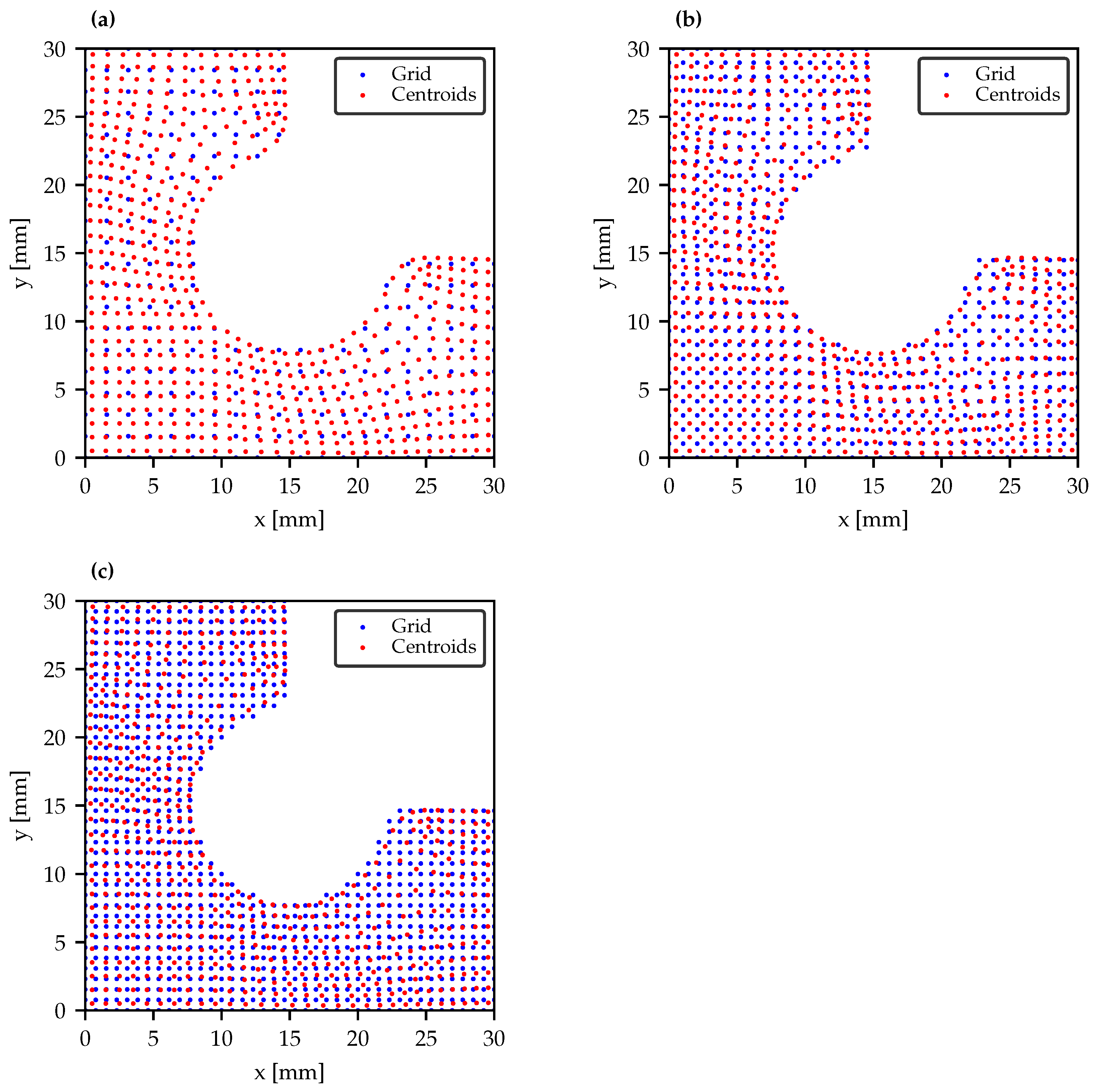
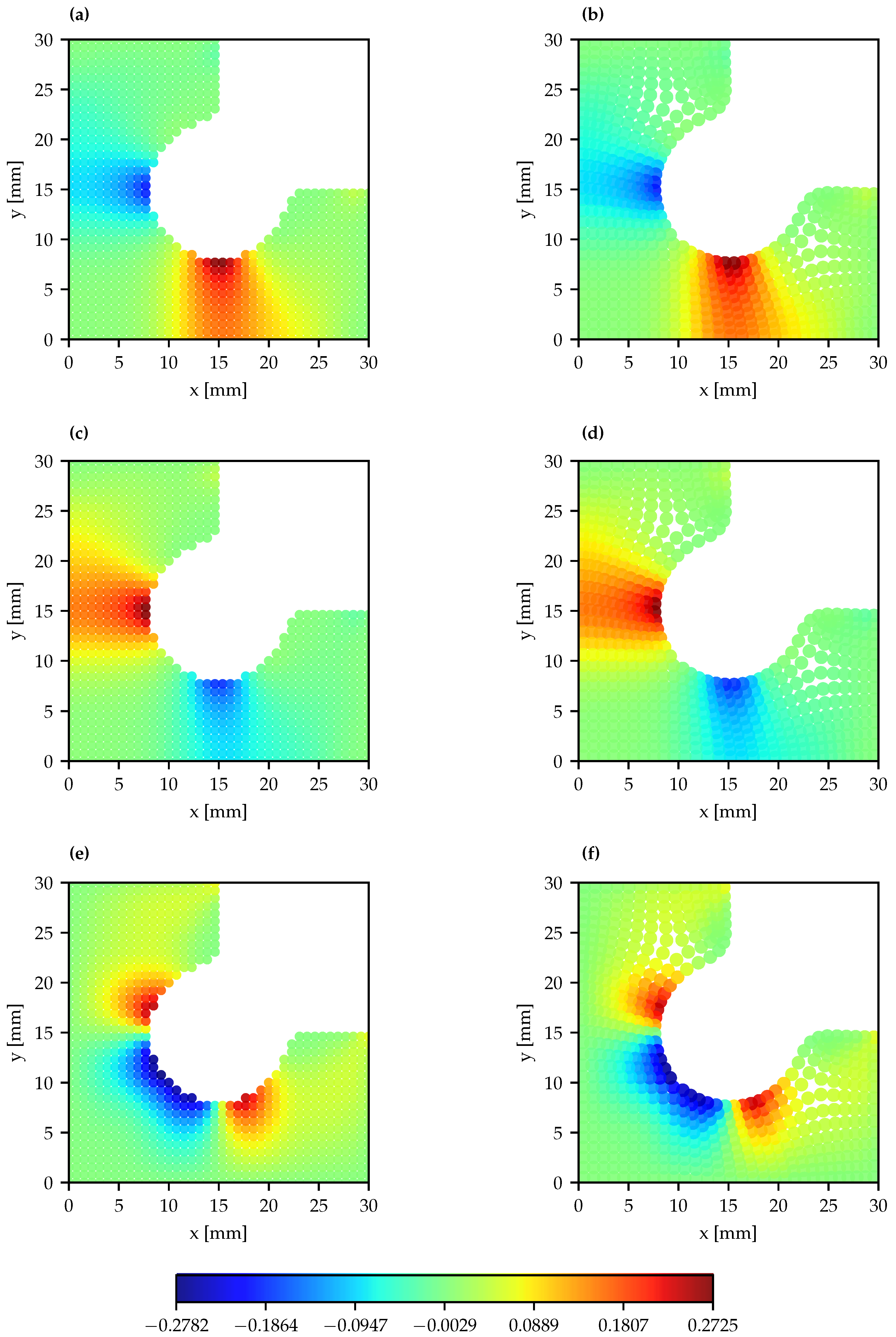
2.4. Interpolation Approach

In order to obtain mesh-independence, this FEA mesh (for training purposes) or DIC subset mesh (for the predict stage) is converted in a grid of points using interpolation. For this approach, Python’s scipy.interpolate library [41] is used, which provides a collection of mathematical algorithms and functions used for performing interpolation tasks, including both univariate and multivariate data interpolation, with support for regular and scattered datasets. Inside this library, the RBFInterpolator (Radial Basis Function Interpolator) class is used as it is particularly suited for scattered data interpolation (i.e., where data points are irregularly distributed in space). Additionally, it supports extrapolation, which is a crucial feature for this use case, as some points are generated near to the sample geometry limits without being fully surrounded by centroids. Previously, griddata class [42] was also explored. However, its applicability for this study is limited since it does not support extrapolation. Inside RBFInterpolator class, the chosen methods are linear, cubic, and multiquadric; more details about this class and its methods can be found in the literature [43].

A regular grid of points is defined within a 30 × 30 mm² bounding square, which represents the cruciform’s shape in-plane dimensions for one-eighth of the sample. From the total number of generated points, only some can fit inside the cruciform’s area (domain). Three regular grids are generated to test different point densities in comparison to the centroids of the finite element mesh. All the values and statistics performed regarding these grids are presented in

Table 3. Total number of generated points, number of points inside the domain, and their relative density compared to the number of mesh centroids, for each grid size.

Grid Size	Total Points	Domain Points	Relative Density
20 × 20	400	253	≈0.45
30 × 30	900	564	1.00
40 × 40	1600	1006	≈1.78

.

Furthermore, Figure 2a, Figure 2b and Figure 2c show the generated grids with resolutions of 20 × 20, 30 × 30, and 40 × 40, respectively, compared to the centroids of the finite element mesh. Only X_train and X_test matrices are interpolated using these methods and grids, performing a total of nine interpolated datasets (three interpolation methods × three grids) for each matrix.

In order to visually check the interpolation results, a comparison between interpolated and original strain values (${ϵ}_{xx}$, ${ϵ}_{yy}$ and ${ϵ}_{xy}$) obtained for the last time-step of the numerical simulation is presented in Figure 3. These results demonstrate the similarity of the compared values, proving the coherence between interpolated and original data.

Before advancing further, the accuracy of each interpolated dataset is evaluated by conducting a reverse interpolation. In this process, interpolated data are re-interpolated back to the original points (centroids) using the same method initially applied, being able to compare results and check which method and grid guarantees the more accurate prediction.

2.5. Training and Evaluation

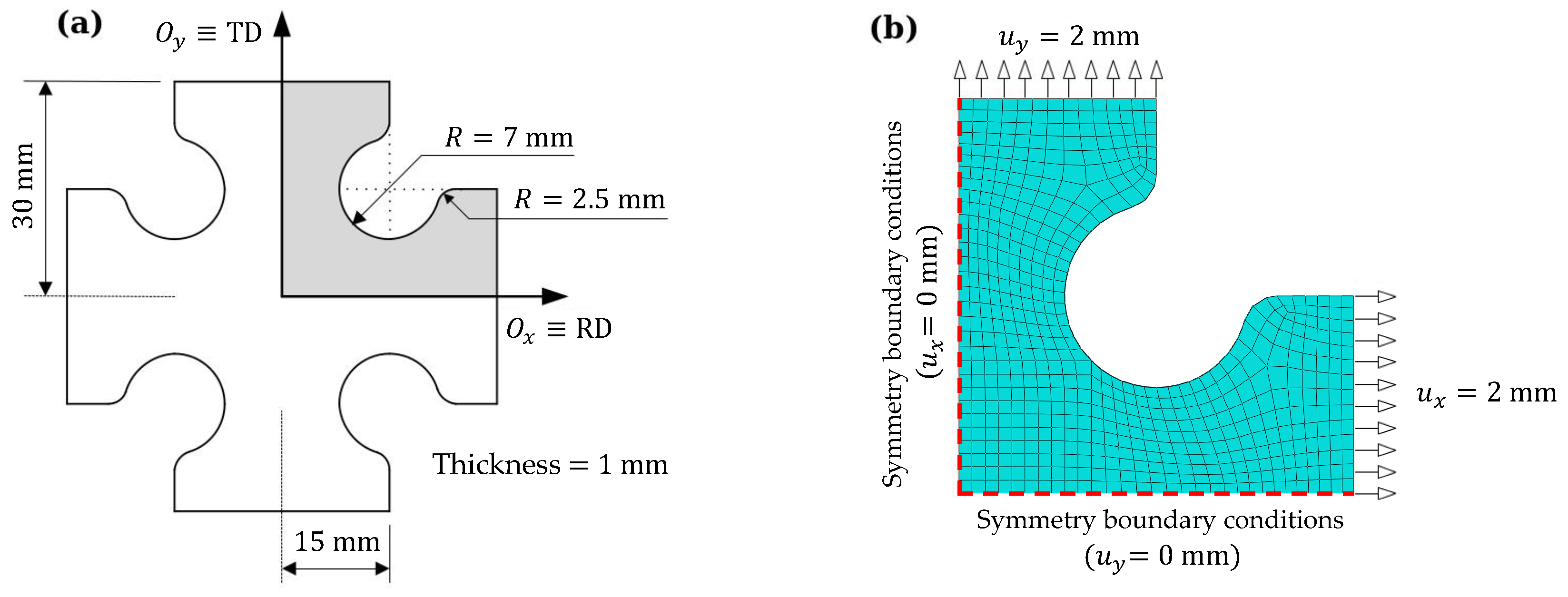
After the interpolation process and evaluation, the XGBoost algorithm [27,28] is trained using the interpolated datasets. The hyperparameters of the XGBoost algorithm were kept as default, except for the learning_rate (=0.02), max_depth (=4) and n_estimators (=1000) [27].

In the first approach, the performance of the trained models in predicting material parameters is evaluated using test datasets interpolated with the same method and grid, referred to as the simple test. Additionally, the robustness of each model is assessed using test datasets interpolated with different methods, referred to as the cross test, resulting in a total of 27 possible evaluation combinations. Both evaluations are detailed in the

Table 4. Model evaluation framework: ‘s’ indicates the simple test (same interpolation method as training), and ‘c’ indicates the cross test (different interpolation method from training).

Training Interpolation Method	Grid Size	Test Interpolation Method
		Linear	Cubic	Multiquadric
Linear	20 × 20	s	c	c
	30 × 30	s	c	c
	40 × 40	s	c	c
Cubic	20 × 20	c	s	c
	30 × 30	c	s	c
	40 × 40	c	s	c
Multiquadric	20 × 20	c	c	s
	30 × 30	c	c	s
	40 × 40	c	c	s

.

Throughout this study, the model’s performance is assessed using R² (Coefficient of Determination), MAE (Mean Absolute Error), and MAPE (Mean Absolute Percentage Error) by comparing the obtained results with the original data. These metrics are obtained using Python’s sklearn.metrics library [44] and can be mathematically represented as follows [45]:

$${\mathrm{R}}^2=1-{\displaystyle \frac{{\sum }_{i=1}^m{(X_i-Y_i)}^2}{{\sum }_{i=1}^m{(\overline{Y}-Y_i)}^2}},$$

(6)

$$\mathrm{MAE}={\displaystyle \frac{1}{m}}\sum _{i=1}^m|X_i-Y_i|,$$

(7)

$$\mathrm{MAPE}={\displaystyle \frac{1}{m}}\sum _{i=1}^m\left|{\displaystyle \frac{Y_i-X_i}{Y_i}}\right|,$$

(8)

where $X_i$ and $Y_i$ are the predicted and actual values, respectively, $\overline{Y}$ represents the mean of the actual values, and m is the total number of samples.

2.6. Case Study

As it is not possible to acquire a sample via DIC, either experimentally or virtually (e.g., using MatchID [10,46]), the practical application of this work is demonstrated using a synthetic approach. This consists of predicting a randomly chosen set of parameters from Y_test matrix and using the corresponding features (from X_test) interpolated to a randomly generated set of speckle pattern points and used as an input to a model. Although mesh effects are less pronounced in the pre-failure regime due to smoother strain fields, the interpolation strategy remains crucial for adapting simulated data to experimental formats such as DIC, where spatial resolutions typically do not align with the original FEM mesh.

The generated speckle pattern is represented in Figure 4, consisting of a set of 5000 randomly distributed points and is intended to approximate the subset density typically found in a DIC-acquired sample. In order to simulate the DIC process, the corresponding features are interpolated to the new set of points using the multiquadric method, resulting in a feature matrix with shape 1 × 300,040 (1 sample × 300,040 features). Further on, for simplification purposes, this interpolated sample shall be called synthetic DIC sample.

Finally, to demonstrate the practical application of this work, the obtained synthetic DIC sample is now interpolated using the 30 × 30 grid with multiquadric interpolation method, which is proved to be the best overall method in this study (see Section 3), and then the previously chosen parameters are predicted using the corresponding trained model. As a term of comparison, these parameters are also predicted using the model trained on the original dataset (i.e., without interpolation).

In order to evaluate this approach, the predicted parameters are visually represented through the evolution of the yield stress (Y) during plastic deformation (Equation (5)), the initial yield stress in tension as a function of loading angle w.r.t. rolling direction, ${\sigma }_0\left(\alpha \right)$ (Equation (4)), and anisotropy coefficient as a function of loading angle w.r.t. rolling direction, $r\left(\alpha \right)$ (Equation (3)).

3. Results and Discussion

Figure 5 presents the reverse interpolation performance metrics, including R² (Figure 5a), MAE (Figure 5b), and MAPE (Figure 5c), for different interpolation methods (linear, cubic, and multiquadric) and grid densities (20 × 20, 30 × 30, and 40 × 40). The results indicate that the cubic and multiquadric methods consistently outperform the linear method. In particular, R² values are higher for these methods, reaching a maximum of 0.999, and increasing with grid density. Conversely, MAE and MAPE values remain low for all methods and grids, with a clear decreasing trend as the number of interpolation points increases. Notably, the linear method exhibits the highest errors, while cubic and multiquadric methods achieve superior accuracy across all grid sizes. These findings confirm that cubic and multiquadric interpolation are preferable for accurate reconstructions. For grid evaluation, selecting a grid with a number of points at least equal to or greater than the number of centroids enhances accuracy in data prediction.

Figure 6 presents the simple test performance evaluation metrics, including R² (Figure 6a), MAE (Figure 6b), and MAPE (Figure 6c) for all the different interpolation methods and grid densities presented before. The results indicate that neither the choice of interpolation method nor grid size significantly impacts the model’s prediction performance. Furthermore, R² remains above 0.99, with no notable differences between methods or grids. Similarly, MAE stays below 1.28 and MAPE below 0.0156, showing minimal variation across different methods and grids. The variation between maximum and minimum values for MAE and MAPE is approximately 0.08 and 0.002, respectively.

Figure 7 compares the predicted parameters obtained both using the 40 × 40 grid multiquadric model with those from a model trained on the original dataset (i.e., without interpolation). The comparison includes the predicted values of F, G, N, ${\sigma }_0$, K and n against the real values from the numerical simulations of the test dataset. As evidenced by the presented R² values, both models exhibit similar prediction performance, demonstrating the strong predictive capability of the model trained with interpolated data.

Figure 8 presents the results of the cross tests for the models interpolated using linear (Figure 8a), cubic (Figure 8b), and multiquadric (Figure 8c) methods, when handling test data interpolated by different methods. To maintain clarity and ease of interpretation, only the R² values are shown for models interpolated. Overall, the cubic and multiquadric models prove to be the most robust. With R² > 0.95, the models demonstrate high robustness in accepting data interpolated by different methods. Cubic and multiquadric models tend to be less compatible with receiving linear interpolated data, and vice versa. However, both these models present the best performance when receiving test data interpolated using each other’s methods. As expected, better performance is achieved when the model and the provided test data share the same interpolation method.

Figure 9 presents the computational time analysis regarding interpolation (Figure 9a) and training (Figure 9b) time, performed in a computer with an Intel(R) Xeon(R) E-2236 @3.40 GHz CPU, 64 Gb of RAM, and 512 Gb SSD disk. The results indicate that computational time depends on both the grid size and the interpolation method, except during training, where it depends only on the grid size. Regarding interpolation, the cubic method exhibits the highest values, while the linear method is the most efficient. As expected, computational time increases with grid size for both interpolation and training. However, unlike interpolation, training time shows only minor variations between methods using the same grid and is primarily dependent on grid size rather than the interpolation method.

Considering the previously presented results regarding accuracy and balancing performance with computational cost, the most advantageous combination for interpolation in the present study is the 30 × 30 grid with the multiquadric method. However, it should be noted that this conclusion is specific to the test conditions considered in this work (i.e., cruciform biaxial tensile test using the Hill’48 constitutive model with Swift hardening) and is not intended to be universally optimal across other mechanical tests or constitutive models.

Regarding the practical case study,

Table 5. Material parameters predicted by the original model and by the synthetic DIC sample together with the model trained with a 30 × 30 grid and multiquadric method, both compared to the chosen reference parameters (y_test).

Data	Parameter
	$\mathit{F}$	$\mathit{G}$	$\mathit{N}$	${\mathit{\sigma }}_{\mathbf{0}}$ [MPa]	$\mathit{K}$ [MPa]	$\mathit{n}$
y_test	0.2495	0.1922	2.3281	160.84	671.78	0.218
original_model	0.2679	0.1953	2.3245	155.32	653.63	0.217
DIC	0.2456	0.1918	2.3906	162.15	652.62	0.221

shows the chosen parameters used as reference (y_test) and those predicted by both the original model and synthetic DIC sample together with the model trained with $30\times 30$ grid and multiquadric method. In addition, Figure 10 presents the predicted material parameters through the representation of the hardening curves (Figure 10a), initial yield stress in tension (Figure 10b), and the anisotropy coefficient (Figure 10c) as a function of the angle, $\alpha$, between the tensile direction and the rolling direction of the sheet. Figure 10d–f represent the errors obtained for the Figure 10a–c, respectively, between both the original model and synthetic DIC sample curves relative to the chosen parameters’ curve. Overall, and in line with the previously discussed results, these findings not only demonstrate the strong predictive performance of the model trained with the 30 × 30 grid and multiquadric interpolation method, but also highlight the success of the applied case study, which effectively exemplifies the practical applicability of the proposed approach. In terms of hardening behaviour, the parameters predicted using the synthetic DIC sample and the model trained with interpolated data result in a curve that closely follows the y_test curve. In fact, both predicted parameter sets produce nearly overlapping curves, with a maximum relative error of less than 4%. For the initial yield stress, a near-perfect overlap is observed between the y_test and the synthetic DIC-based predicted parameters, with a maximum relative error of less than 2%. The original model’s predictions yield a curve with a similar shape but a slightly larger deviation, resulting in a maximum relative error below 5%. Finally, regarding the anisotropy coefficient, both sets of predicted parameters generate curves with very similar curvature to the reference, although with a slight offset. Nonetheless, both remain in close proximity to the y_test curve, with maximum relative errors below 5% for the synthetic DIC sample with 30 × 30 grid multiquadric model and below 8% for the original model.

4. Conclusions

Expanding the dataset coverage and reduce the ML model’s dependency on discrete mesh points is a promising issue, as it ensures a more comprehensive model without depending on the mesh discretisation process. In this work, various interpolation methods and grids of points are applied to the generated datasets in order to train ML models and evaluate their performance regarding the prediction of material parameters. Conclusions are as follows:

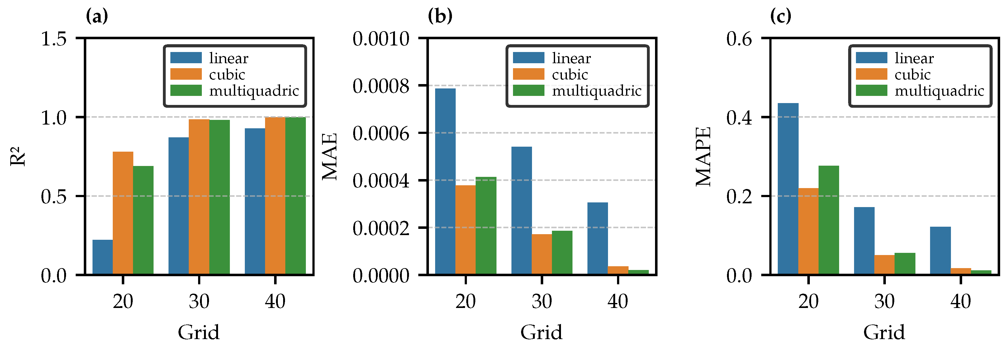
• Interpolation accuracy improves with grid size, with cubic and multiquadric methods outperforming the linear method;
• In reverse interpolation, choosing a grid with at least as many points as the number of mesh centroids improves strain field reconstruction accuracy. However, this increase in grid density has negligible effect on the predictive performance of the ML models;
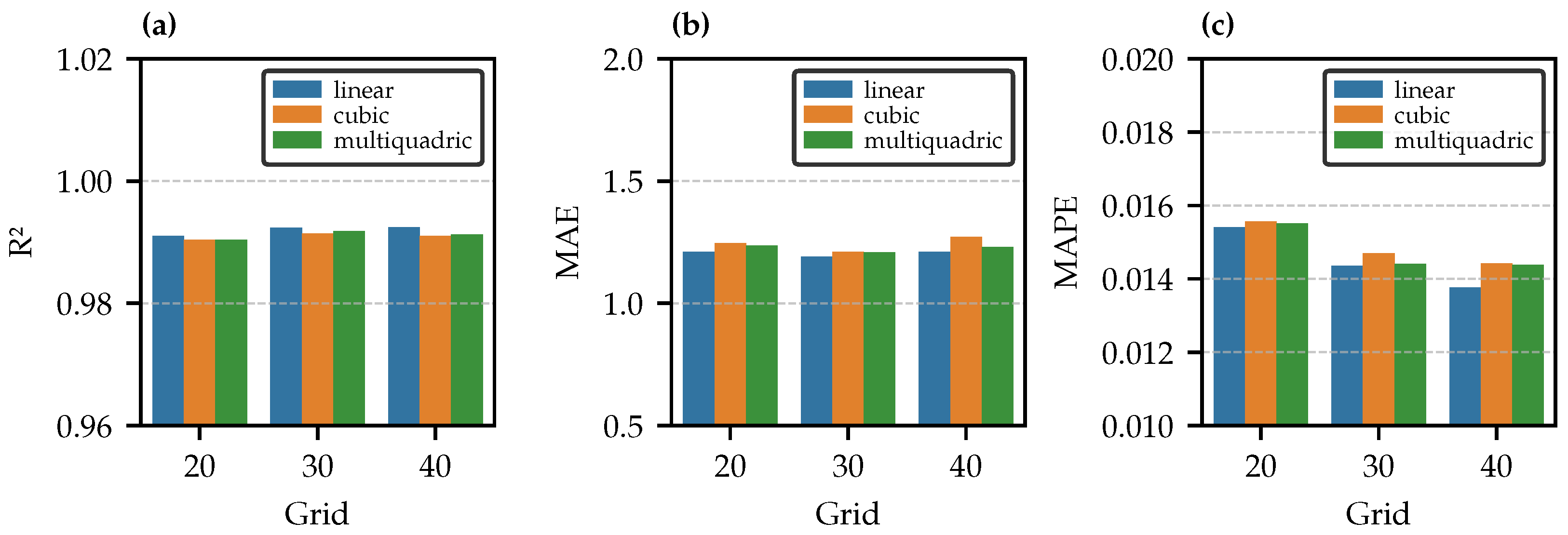
• ML models exhibit strong predictive performance, with the choice of interpolation method or grid having minimal impact on overall model accuracy;
• Similar R² values between models trained on interpolated vs. original data suggest that interpolation does not degrade predictive performance;
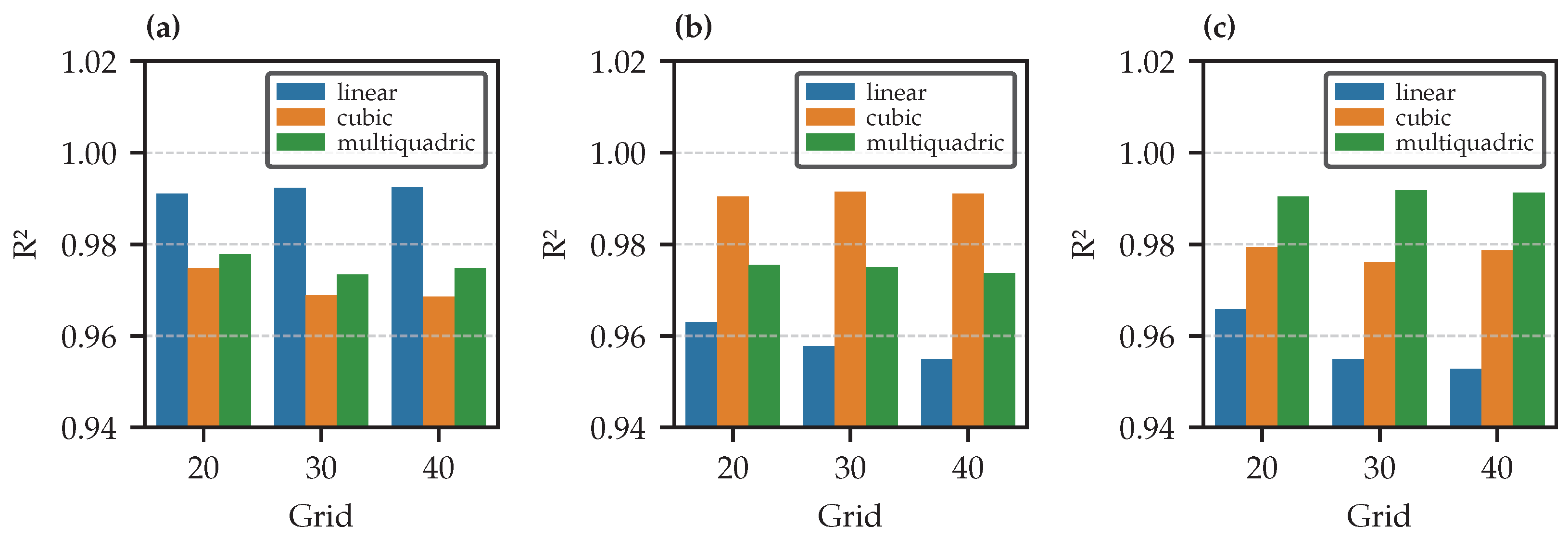
• Models demonstrate high robustness when handling data interpolated by different methods, with cubic and multiquadric models proving the most reliable;
• Cubic and multiquadric models are less compatible with linear-interpolated test data, and vice versa, but perform best when tested with each other’s interpolation methods;
• Better performance is achieved when the model and test data share the same interpolation method;
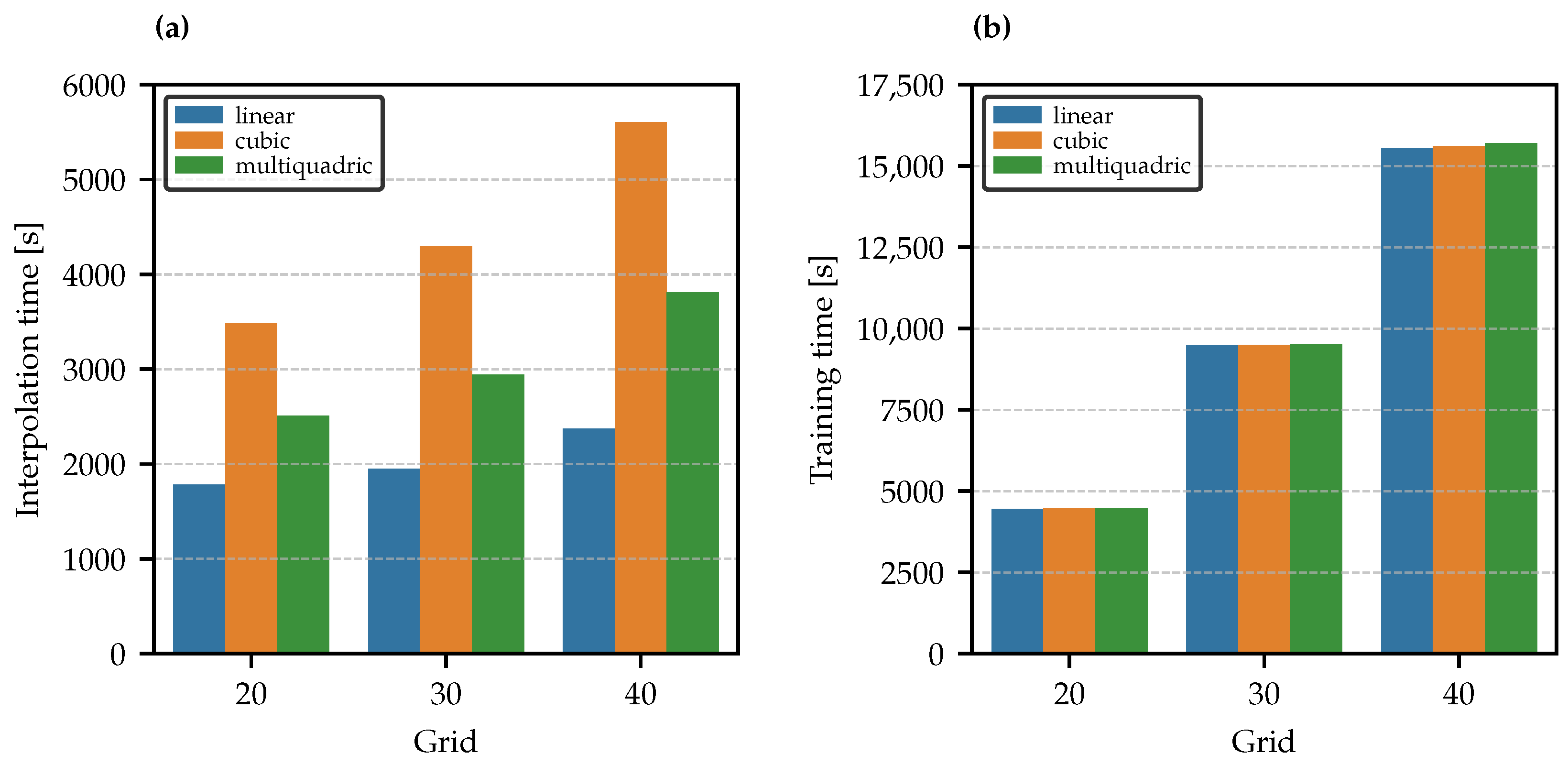
• In terms of computational efficiency, the linear method is the fastest for interpolation, while the cubic method is the most demanding. However, the interpolation method does not affect training time;
• As expected, computational time increases with grid size for both interpolation and training;
• Balancing accuracy, performance, and computational cost, the optimal choice in the present study is the 30 × 30 grid with the multiquadric method. However, this conclusion is specific to the considered setup and should not be generalised without further validation under different constitutive models or testing conditions;
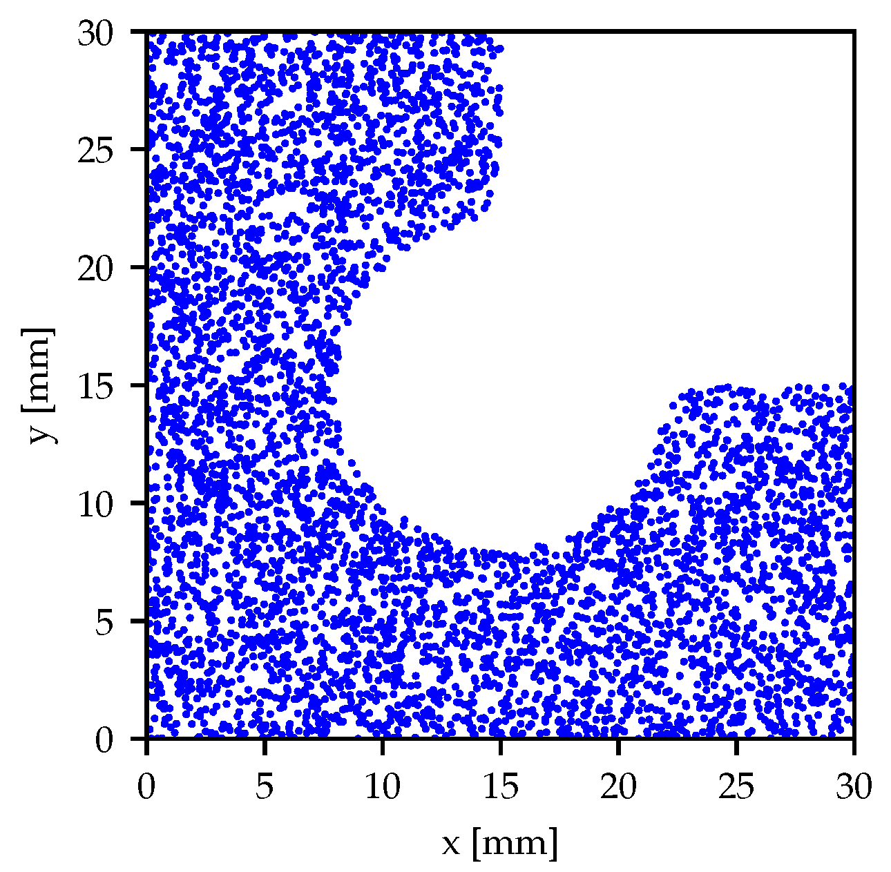
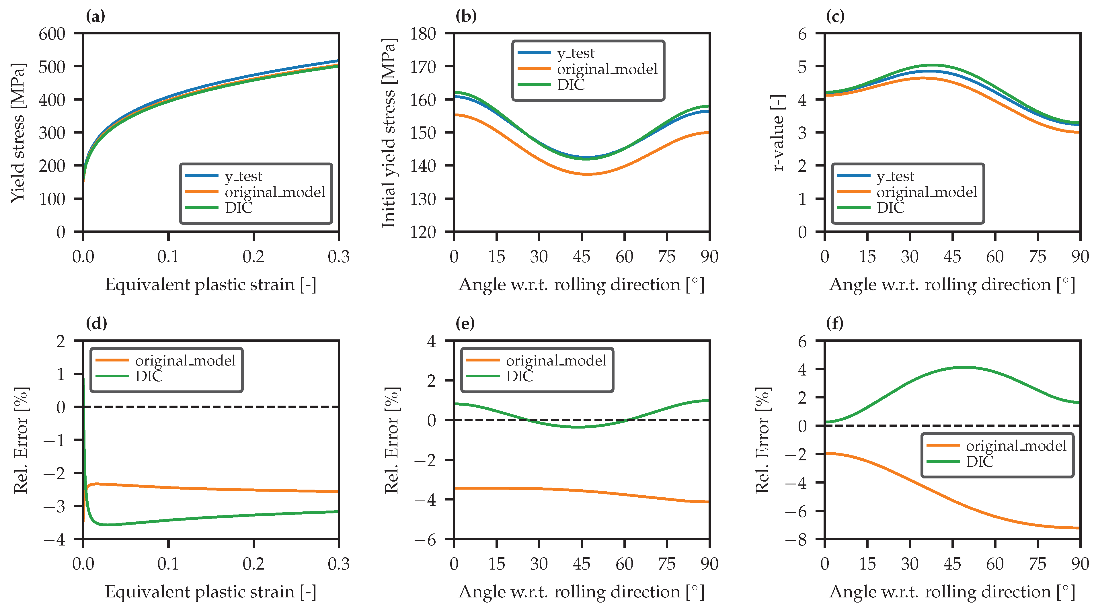
• Synthetic DIC sample predicted parameters closely match those obtained by the original model and the chosen parameters, which not only confirms the strong predictive capability of the model trained with the 30 × 30 grid and multiquadric method, but also demonstrates the effectiveness of the interpolation-based approach when applied to a denser group of points, simulating DIC speckle pattern subsets;
• This study focuses on the pre-failure regime, where strain distributions are relatively smooth. While this condition reduces the severity of mesh dependence, the proposed approach still plays a critical role in enabling compatibility between FEM simulations and full-field experimental data (e.g., DIC), which are often collected with non-matching spatial resolutions.

For future research, a more detailed exploration of alternative interpolation methods is recommended. Additionally, a grid variation study could provide insights into potential trends or patterns. Investigating the use of disperse points instead of a regular grid may offer a valuable perspective on the impact of spatial distribution. Furthermore, applying the proposed methodology to real DIC-acquired samples is suggested to assess its performance in experimental settings. Although this work focuses on pre-failure regimes, extending this approach to post-necking conditions could be an important future research, where mesh dependence may be more pronounced. Moreover, the optimal interpolation strategy identified here is specific to the studied case and requires further validation for other tests and models.

References

1. do Nascimento Cruz, M.; Nikhare, C.; Filho, R.; Marcondes, P. Sheet metal formability analysis by accessible and reliable digital image correlation system. Int. J. Adv. Manuf. Technol. 2025, 137, 2307–2317. [Google Scholar] [CrossRef]
2. Parreira, T.G.; Marques, A.E.; Sakharova, N.A.; Prates, P.A.; Pereira, A.F.G. Identification of Sheet Metal Constitutive Parameters Using Metamodeling of the Biaxial Tensile Test on a Cruciform Specimen. Metals 2024, 14, 212. [Google Scholar] [CrossRef]
3. Diller, M.; Thomas, W.; Ahmetoglu, M.A.; Akgerman, N.; Altan, T.; Diller, M.; Thomas, W.; Ahmetoglu, M.A.; Akgerman, N.; Altan, T. Applications of Computer Simulations for Part and Process Design for Automotive Stampings; SAE International: Warrendale, PA, USA, 1997. [Google Scholar] [CrossRef]
4. Yoshida, F.; Hamasaki, H.; Uemori, T. A user-friendly 3D yield function to describe anisotropy of steel sheets. Int. J. Plast. 2013, 45, 119–139. [Google Scholar] [CrossRef]
5. Chaparro, B.M.; Thuillier, S.; Menezes, L.F.; Manach, P.Y.; Fernandes, J.V. Material parameters identification: Gradient-based, genetic and hybrid optimization algorithms. Comput. Mater. Sci. 2008, 44, 339–346. [Google Scholar] [CrossRef]
6. Fu, J.; Cai, Y.; Zhang, B.; Qi, Z.; Liu, F.; Qi, L. A VFM-based identification method for anisotropic thermal-mechanical properties of sheet metals using the digital image correlation and infrared thermography assisted heterogeneous test. J. Mater. Process. Technol. 2024, 330, 118490. [Google Scholar] [CrossRef]
7. Rabahallah, M.; Balan, T.; Bouvier, S.; Bacroix, B.; Barlat, F.; Chung, K.; Teodosiu, C. Parameter identification of advanced plastic strain rate potentials and impact on plastic anisotropy prediction. Int. J. Plast. 2009, 25, 491–512. [Google Scholar] [CrossRef]
8. Avril, S.; Bonnet, M.; Bretelle, A.S.; Grédiac, M.; Hild, F.; Ienny, P.; Latourte, F.; Lemosse, D.; Pagano, S.; Pagnacco, E.; et al. Overview of Identification Methods of Mechanical Parameters Based on Full-field Measurements. Exp. Mech. 2008, 48, 381–402. [Google Scholar] [CrossRef]
9. Rossi, M.; Lattanzi, A.; Amodio, D. A hybrid VFM-FEMU approach to calibrate 3D anisotropic plasticity models for sheet metal forming. Mater. Res. Proc. 2023, 28, 1203–1210. [Google Scholar] [CrossRef]
10. Zhang, Y.; Yamanaka, A.; Cooreman, S.; Kuwabara, T.; Coppieters, S. Inverse identification of plastic anisotropy through multiple non-conventional mechanical experiments. Int. J. Solids Struct. 2023, 285, 112534. [Google Scholar] [CrossRef]
11. Chen, B.; Starman, B.; Halilovič, M.; Berglund, L.A.; Coppieters, S. Finite Element Model Updating for Material Model Calibration: A Review and Guide to Practice. Arch. Comput. Methods Eng. 2024. [Google Scholar] [CrossRef]
12. Fu, J.; Xie, W.; Qi, L. An Identification Method for Anisotropic Plastic Constitutive Parameters of Sheet Metals. Procedia Manuf. 2020, 47, 812–815. [Google Scholar] [CrossRef]
13. Fu, J.; Yang, Z.; Nie, X.; Tang, Y.; Cai, Y.; Yin, W.; Qi, L. A VFM-based identification method for the dynamic anisotropic plasticity of sheet metals. Int. J. Mech. Sci. 2022, 230, 107550. [Google Scholar] [CrossRef]
14. Lattanzi, A.; Barlat, F.; Pierron, F.; Marek, A.; Rossi, M. Inverse identification strategies for the characterization of transformation-based anisotropic plasticity models with the non-linear VFM. Int. J. Mech. Sci. 2020, 173, 105422. [Google Scholar] [CrossRef]
15. Florentin, E.; Lubineau, G. Identification of the parameters of an elastic material model using the constitutive equation gap method. Comput. Mech. 2010, 46, 521–531. [Google Scholar] [CrossRef]
16. Latourte, F.; Chrysochoos, A.; Pagano, S.; Wattrisse, B. Elastoplastic Behavior Identification for Heterogeneous Loadings and Materials. Exp. Mech. 2008, 48, 435–449. [Google Scholar] [CrossRef]
17. Claire, D.; Hild, F.; Roux, S. A finite element formulation to identify damage fields: The equilibrium gap method. Int. J. Numer. Methods Eng. 2004, 61, 189–208. [Google Scholar] [CrossRef]
18. Périé, J.N.; Leclerc, H.; Roux, S.; Hild, F. Digital image correlation and biaxial test on composite material for anisotropic damage law identification. Int. J. Solids Struct. 2009, 46, 2388–2396. [Google Scholar] [CrossRef]
19. Cruz, D.J.; Barbosa, M.R.; Santos, A.D.; Amaral, R.L.; de Sa, J.C.; Fernandes, J.V. Recurrent Neural Networks and Three-Point Bending Test on the Identification of Material Hardening Parameters. Metals 2024, 14, 84. [Google Scholar] [CrossRef]
20. Kim, J.; Ebrahim, A.S.; Kinsey, B.L.; Ha, J. Identification of Yld2000–2d anisotropic yield function parameters from single hole expansion test using machine learning. CIRP Ann. 2024, 73, 233–236. [Google Scholar] [CrossRef]
21. Böhringer, P.; Sommer, D.; Haase, T.; Barteczko, M.; Sprave, J.; Stoll, M.; Karadogan, C.; Koch, D.; Middendorf, P.; Liewald, M. A strategy to train machine learning material models for finite element simulations on data acquirable from physical experiments. Comput. Methods Appl. Mech. Eng. 2023, 406, 115894. [Google Scholar] [CrossRef]
22. Chamekh, A.; BelHadjSalah, H.; Hambli, R.; Gahbiche, A. Inverse identification using the bulge test and artificial neural networks. J. Mater. Process. Technol. 2006, 177, 307–310. [Google Scholar] [CrossRef]
23. Chamekh, A.; Bel Hadj Salah, H.; Hambli, R. Inverse technique identification of material parameters using finite element and neural network computation. Int. J. Adv. Manuf. Technol. 2009, 44, 173–179. [Google Scholar] [CrossRef]
24. Jang, D.P.; Fazily, P.; Yoon, J.W. Machine learning-based constitutive model for J2- plasticity. Int. J. Plast. 2021, 138, 102919. [Google Scholar] [CrossRef]
25. Guo, Y.; Wang, C.; Han, S.; Kosec, G.; Zhou, Y.; Wang, L.; Abdel Wahab, M. A deep neural network model for parameter identification in deep drawing metal forming process. J. Manuf. Process. 2025, 133, 380–394. [Google Scholar] [CrossRef]
26. Stefanovska, E.; Pepelnjak, T. Optimising predictive accuracy in sheet metal stamping with advanced machine learning: A LightGBM and neural network ensemble approach. Adv. Eng. Inform. 2025, 65, 103103. [Google Scholar] [CrossRef]
27. Chen, T.; Guestrin, C. XGBoost: A Scalable Tree Boosting System. In Proceedings of the 22nd ACM SIGKDD International Conference on Knowledge Discovery and Data Mining, San Francisco, CA, USA, 13–17 August 2016; KDD ’16; Association for Computing Machinery: New York, NY, USA, 2016; pp. 785–794. [Google Scholar] [CrossRef]
28. Andrade-Campos, A.; Bastos, N.; Conde, M.; Gonçalves, M.; Henriques, J.; Lourenço, R.; Martins, J.M.P.; Oliveira, M.G.; Prates, P.; Rumor, L. On the inverse identification methods for forming plasticity models using full-field measurements. IOP Conf. Ser. Mater. Sci. Eng. 2022, 1238, 012059. [Google Scholar] [CrossRef]
29. Bastos, N.; Prates, P.A.; Andrade-Campos, A. Material Parameter Identification of Elastoplastic Constitutive Models Using Machine Learning Approaches. Key Eng. Mater. 2022, 926, 2193–2200. [Google Scholar] [CrossRef]
30. Prates, P.; Pinto, J.; Marques, J.; Henriques, J.; Pereira, A.; Andrade-Campos, A. Influence of data filtering and noise on the calibration of constitutive models using machine learning techniques. Mater. Form. 2024, 41, 1807–1816. [Google Scholar] [CrossRef]
31. Xia, J.; Won, C.; Kim, H.; Lee, W.; Yoon, J. Artificial Neural Networks for Predicting Plastic Anisotropy of Sheet Metals Based on Indentation Test. Materials 2022, 15, 1714. [Google Scholar] [CrossRef]
32. Reu, P.L.; Blaysat, B.; Andó, E.; Bhattacharya, K.; Couture, C.; Couty, V.; Deb, D.; Fayad, S.S.; Iadicola, M.A.; Jaminion, S.; et al. DIC Challenge 2.0: Developing Images and Guidelines for Evaluating Accuracy and Resolution of 2D Analyses. Exp. Mech. 2022, 62, 639–654. [Google Scholar] [CrossRef]
33. Chen, B.; Coppieters, S. Unified digital image correlation under meshfree framework. Strain 2024, 60, e12461. [Google Scholar] [CrossRef]
34. Prates, P.A.; Pereira, A.F.G.; Sakharova, N.A.; Oliveira, M.C.; Fernandes, J.V. Inverse Strategies for Identifying the Parameters of Constitutive Laws of Metal Sheets. Adv. Mater. Sci. Eng. 2016, 2016, 4152963. [Google Scholar] [CrossRef]
35. Martins, J.M.P.; Andrade-Campos, A.; Thuillier, S. Calibration of anisotropic plasticity models using a biaxial test and the virtual fields method. Int. J. Solids Struct. 2019, 172–173, 21–37. [Google Scholar] [CrossRef]
36. Prates, P. Coupling machine learning and synthetic image DIC-based techniques for the calibration of elastoplastic constitutive models. Mater. Form. 2023, 28, 1193–1202. [Google Scholar] [CrossRef]
37. Dassault Systèmes. Abaqus 2016 Analysis User’s Guide; Dassault Systèmes Simulia Corp.: Providence, RI, USA, 2016; Volume 1–5. [Google Scholar]
38. Hill, R.; Orowan, E. A theory of the yielding and plastic flow of anisotropic metals. Proc. R. Soc. London. Ser. A Math. Phys. Sci. 1948, 193, 281–297. [Google Scholar] [CrossRef]
39. Swift, H.W. Plastic instability under plane stress. J. Mech. Phys. Solids 1952, 1, 1–18. [Google Scholar] [CrossRef]
40. Randomized Designs—pyDOE3 1.0.4.dev3 Documentation. Available online: https://pydoe3.readthedocs.io/en/latest/randomized.html#latin-hypercube (accessed on 7 March 2025).
41. Interpolation (scipy.interpolate)—SciPy v1.15.2 Manual. Available online: https://docs.scipy.org/doc/scipy/reference/interpolate.html (accessed on 4 March 2025).
42. Griddata—SciPy v1.15.2 Manual. Available online: https://docs.scipy.org/doc/scipy/reference/generated/scipy.interpolate.griddata.html#scipy.interpolate.griddata (accessed on 4 March 2025).
43. RBFInterpolator—SciPy v1.15.2 Manual. Available online: https://docs.scipy.org/doc/scipy/reference/generated/scipy.interpolate.RBFInterpolator.html#scipy.interpolate.RBFInterpolator (accessed on 4 March 2025).
44. Metrics and Scoring: Quantifying the Quality of Predictions. Available online: https://scikit-learn.org/stable/modules/model_evaluation.html (accessed on 9 March 2025).
45. Chicco, D.; Warrens, M.J.; Jurman, G. The coefficient of determination R-squared is more informative than SMAPE, MAE, MAPE, MSE and RMSE in regression analysis evaluation. PeerJ Comput. Sci. 2021, 7, e623. [Google Scholar] [CrossRef]
46. Lava, P.; Jones, E.M.C.; Wittevrongel, L.; Pierron, F. Validation of finite-element models using full-field experimental data: Levelling finite-element analysis data through a digital image correlation engine. Strain 2020, 56, e12350. [Google Scholar] [CrossRef]
Figure 1. Biaxial tensile test on a cruciform sample, adapted from Ref. [30]: (a) geometry and dimensions; (b) boundary conditions and finite element mesh.
Metals 15 00534 g001
Figure 2. Comparison of generated grid points and finite element centroids: (a) 20 × 20 grid; (b) 30 × 30 grid; (c) 40 × 40 grid.
Metals 15 00534 g002
Figure 3. Comparison between the original and interpolated strain fields on a 40 × 40 grid using the multiquadric method, obtained at the last time step: (a) ϵ x x interpolated; (b) ϵ x x original; (c) ϵ y y interpolated; (d) ϵ y y original; (e) ϵ x y interpolated; (f) ϵ x y original.
Metals 15 00534 g003
Figure 4. Randomly obtained speckle pattern with 5000 points.
Metals 15 00534 g004
Figure 5. Reverse interpolation metrics: (a) R2; (b) MAE; (c) MAPE.
Metals 15 00534 g005
Figure 6. Simple test performance evaluation metrics: (a) R2; (b) MAE; (c) MAPE.
Metals 15 00534 g006
Figure 7. Comparison between the predicted constitutive parameters obtained both using the 40 × 40 grid multiquadric model (figures with black dots) and a model trained with the original dataset (figures with blue dots).
Metals 15 00534 g007
Figure 8. Cross test performance evaluation metrics: (a) R2 for linear model; (b) R2 for cubic model; (c) R2 for multiquadric model.
Metals 15 00534 g008
Figure 9. Computational time metrics: (a) interpolation; (b) training.
Metals 15 00534 g009
Figure 10. Comparison of predicted material responses and relative errors using three sets of constitutive parameters: (a) yield stress as a function of equivalent plastic strain (hardening); (b) initial yield stress in tension as a function of α ; (c) anisotropic coefficient evolution as a function of α ; (df) errors obtained for the data presented in (ac), respectively, between both the original model and synthetic DIC sample curves relative to the chosen parameters’ curve.
Metals 15 00534 g010