Detection of Q235 Mild Steel Resistance Spot Welding Defects Based on EMD-SVM

Abstract

Real-time detection of welding defects in resistance spot welding is a complex challenge. Dynamic resistance (DR) reflects nugget growth and varies with defect types, serving as a key indicator. This study presents an online quality evaluation and defect classification method for Q235 low-carbon steel welding. Welding current and voltage were collected in real-time, and DR signals were processed employing a second-order Butterworth low-pass filter featuring zero-phase processing to enhance accuracy. Empirical mode decomposition (EMD) decomposed these signals into intrinsic mode functions (IMFs) and residuals, which were classified by a support vector machine (SVM). Experiments showed the EMD-SVM method outperforms traditional approaches, including backpropagation (BP) neural networks, SVM, wavelet packet decomposition (WPD)-BP, WPD-SVM, and EMD-BP, in identifying four welding states: normal, spatter, false, and edge welding. This method provides an efficient, robust solution for online defect detection in resistance spot welding.

1. Introduction

Resistance spot welding (RSW) is a type of metal connection technology. It operates by the following mechanism: through an industrial AC power supply, after the transformer boosts the voltage and increases the current, welding pressure is exerted on the joint by the electrodes. The current flows through the contact surface of the joint and the adjacent area, generating resistance heat to melt the local metal, ultimately achieving a metallurgical combination of the workpiece [1].

RSW delivers key benefits like high efficiency, consistent quality, cost savings, and automation readiness [2]. Widely used in automotive and industrial applications, it effectively joins steel, aluminum, copper, and their alloys [3]. However, abnormal conditions such as poor surface quality and positioning deviation of the workpiece can lead to fluctuations in the size of the nugget, causing defects such as false welding, burning through, surface spattering and edge welding, which seriously affect the welding strength and safety [4]. Traditional welding quality assessment methods, such as stripping, shearing and shear strength tests, are destructive and inefficient and waste materials [5]. Therefore, non-destructive testing technology has gradually become a research hotspot [6,7]. Scholars extract signals from physical phenomena such as electricity, magnetism, force, sound, and light during the dynamic welding process, enabling non-destructive and real-time monitoring of welding quality [7]. With the advancement of machine vision and machine learning technologies, non-contact detection using image processing and intelligent algorithms provides a new solution for welding defect identification [8,9] that enhances detection accuracy and real-time performance, facilitating spot welding quality control.

This study employs Q235 low-carbon steel for resistance spot welding defect experiments due to its extensive use in automotive, construction, and mechanical industries [10]. With a low carbon content, high weldability, and yield strength of approximately 235 MPa, Q235 offers excellent plasticity and welding performance. Its low carbon content suppresses hardened structure formation, moderate resistivity, and low thermal conductivity while reducing welding energy consumption, and a wide plastic temperature range with a narrow crystallization interval minimizes hot cracking. As the most widely used engineering steel, Q235’s cost effectiveness and process compatibility provide a representative sample for studying the impact of welding parameters on joint quality, offering practical guidance for optimizing spot welding in manufacturing.

During the welding operation, some signals generated during the welding process have a strong correlation accompanying the nucleation and growth of the weld nugget [11]; typical signals include electrode displacement signals, electrode pressure signals, dynamic resistance signals, etc. The variations in these signals clearly indicate the nugget’s growth process. The characteristics of these signals serve as a means for determining defects in the welding process, such as welding problems like spatter. Meanwhile, changes in the welding power curve can also provide important clues to help identify surface or potential defects. By analyzing these signals, the welding process can be predicted and monitored more accurately, and the precision and efficiency of welding quality control can be improved [12,13].

Welding signal analysis usually relies on feature extraction and classification methods, including time-domain, frequency-domain, and time-frequency analysis. However, in the face of complex signals, traditional classification methods (such as threshold method or simple statistical method) have difficulties in high accuracy and real-time performance. The instantaneous and closed welding process makes the limitations of existing methods more prominent. Artificial feature extraction (such as peak value, slope, etc.) is subjective and limits model generalization due to complex signal dynamics. Thus, traditional methods struggle to address variable welding defects and achieve adaptive online quality assessment.

To overcome traditional methods’ limitations, research is increasingly focusing on the optimization of signal preprocessing and classification algorithms [14,15]. Techniques like wavelet packet decomposition, Fourier transform, and Hilbert–Huang transform (HHT) efficiently extract time-frequency features from welding signals, enhancing recognition accuracy. HHT, based on empirical mode decomposition (EMD), adaptively decomposes non-stationary signals into intrinsic mode functions (IMFs), accurately capturing transient characteristics and overcoming wavelet transform’s reliance on predefined functions [16,17]. For classification, support vector machine (SVM) constructs an optimal hyperplane in high-dimensional space using kernel functions, excelling in small-sample, high-dimensional scenarios. The EMD-SVM model combines the multi-resolution analysis of EMD and the high-dimensional classification advantages of SVM, extracting key IMF components and reducing dimensions. This allows for effective capture of signal details and reveals the multi-level information of transient signals. Compared to traditional methods, EMD-SVM shows better adaptability in detecting complex welding defects. It captures transient variations across multiple frequency bands, helping to identify defects that might be missed by conventional approaches. The method reduces redundant features, streamlining analysis and improving classification accuracy, leading to more reliable results and higher weld integrity.

In this work, a signal acquisition quality assessment platform is established, and a reliable real-time evaluation method for welding defect detection is proposed. By analyzing the differences in dynamic resistance signals under various welding defects, the reliability of detecting welding defects using dynamic resistance characteristics is studied. To enhance detection accuracy and generalization ability, a welding defect detection model based on EMD-SVM is proposed. The adaptive decomposition capability of EMD allows the model to extract multi-scale dynamic features of different defects in the welding process without relying on fixed parameter settings, enabling robust adaptation to diverse welding conditions and defect types. SVM leverages its efficient classification ability to model complex nonlinear relationships, accurately classifying signal features processed by EMD to identify defect types. The novelty of the EMD-SVM model lies in its tailored integration for welding defect detection, optimizing EMD’s adaptive decomposition to capture the unique dynamic resistance characteristics of welding signals and enhancing SVM’s classification for welding-specific nonlinear patterns. Unlike prior EMD-SVM applications in other fields, such as fault diagnosis or medical signal processing, this model is specifically designed to address the challenges of real-time welding quality assessment, offering superior sensitivity and adaptability to complex welding environments. This innovative EMD-SVM model demonstrates significant advantages in improving detection accuracy and broadening application scope. It can be extended to monitor and process other industrial signals, providing an efficient and reliable technical path for welding quality control and broader industrial inspection.

2. Experimental Apparatus and Signal Filtering

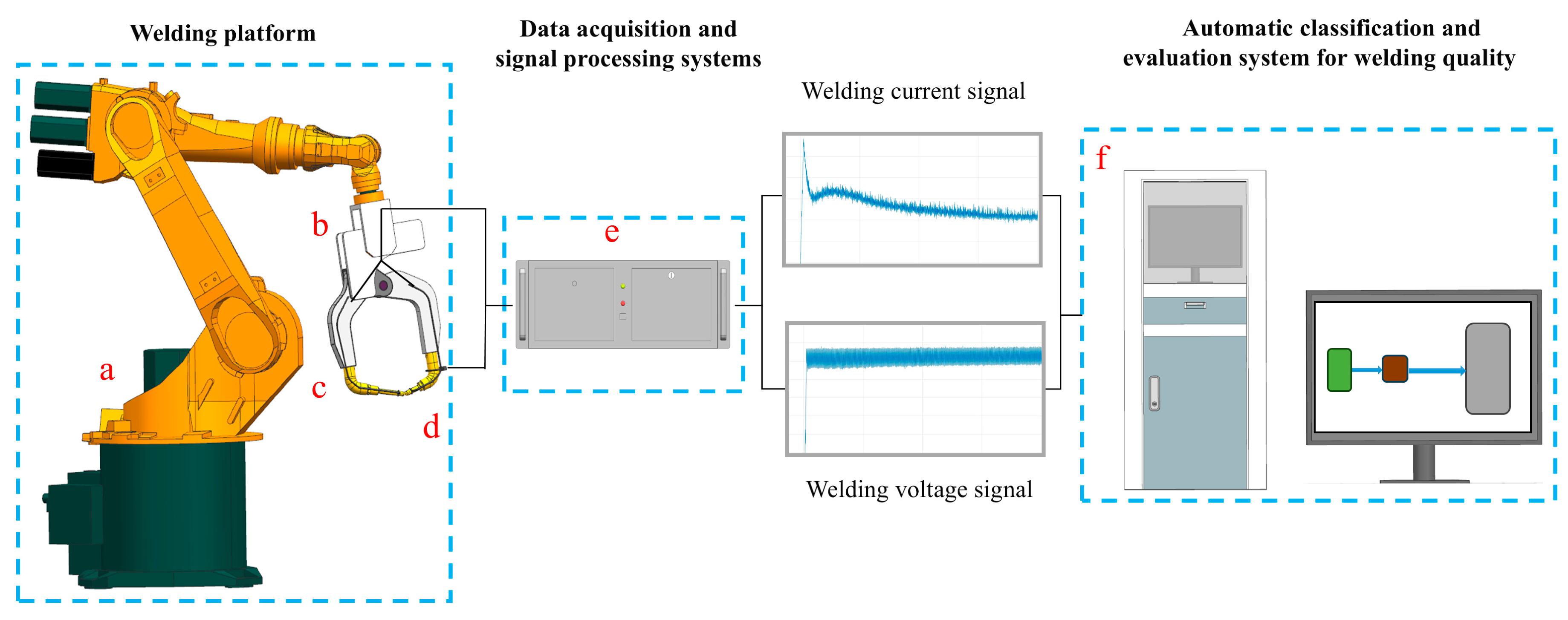
2.1. Experimental Device and Experimental Design

The experimental material is 0.8 mm thick Q235 mild steel.

Table 1. Chemical composition of applied steel sheet (mass %).

Steel Grades	C	Mn	Si	S	P
Q235	<0.22	<1.40	<0.35	<0.045	<0.045

shows the chemical composition of Q235 mild steel. The welding experiment system platform is depicted in Figure 1, which is mainly composed of the following modules:

A medium-frequency direct current (MFDC) welding gun was employed as the welding actuator. A six-axis high-precision welding robot ensures accurate weld point positioning and trajectory control. The MFDC spot welding machine converts AC signals into pulsating DC signals, with a frequency range of 1 kHz to 10 kHz. In this study, the controller operated at an output frequency of 1000 Hz [18]. The current sensor utilizes a Rogowski coil, operating on the principle of electromagnetic induction, with a measurement bandwidth of 1 Hz to 1 MHz and a current range of 1 A to 100 kA, offering high measurement accuracy. Integrated into the medium-frequency DC spot welding system described earlier, it enables non-contact measurement of dynamic welding current signals. This sensor provides several advantages, including galvanic isolation, suitability for high-current detection, compact size, and cost effectiveness, making it ideal for precise and reliable welding quality monitoring [19]. A double-shielded twisted-pair voltage sensor can effectively suppress electromagnetic interference and guarantee signal fidelity. The system incorporates a high-speed synchronous PCI data acquisition card (HK PCI-v6573) operating at a 100 kHz sampling rate, capturing 100,000 signal points per second. The control core of the system adopts the real-time control architecture based on an industrial computer to achieve simultaneous collection of welding voltage and current signals from the resistance spot welding gun and then carries out data feature extraction and welding quality classification.

As can be seen in Figure 1, the welding procedure monitoring experimental platform built in this study synchronously gathers real-time voltage and current signals of the welding process through current sensors (c) and voltage sensors (b) arranged in closed-loop, and completes analog to digital conversion processing through a high-precision multi-channel data acquisition card (e) and transmits digital signals to the control system (f). In this system, the time domain alignment and noise suppression of the original electrical signal are implemented by filtering algorithm, and the dynamic resistance characteristic curve is reconstructed in real time by Ohm’s law. Lastly, a composite classification algorithm leveraging multi-feature integration was implemented to identify the pattern of the dynamic resistance signal curve during welding, enabling quality assessment of solder joints and evaluation of process reliability.

Preliminary experiments were performed on Q235 steel samples using the previously described medium-frequency DC spot welding system to acquire coarse data on weld quality. These initial tests utilized visual inspection, weld nugget diameter measurement, and tensile destructive testing to identify conditions prone to defects, including spatter, false welding, and edge welding. Based on these findings, a tailored defect testing plan was developed for subsequent experiments, as outlined below, to systematically investigate defect formation under optimized welding conditions.

This paper examines prevalent defects in the production process, including spatter, false welding, and edge welding:

(1)

Welding spatter experiment: This experiment aimed to study the conditions of sputtering and side welding. The electrode contact surface diameter was 6 mm, and the welding current was adjusted to 9 kA, with a welding duration of 280 ms. Studies have shown that under the above parameters, lower pressures (such as 2.5 kN) are more likely to lead to spatter defects. To further examine the effect of pressure on spatter occurrence, two distinct pressure levels, 2.5 kN and 3 kN, were evaluated;

(2)

False welding experiment: Under the conditions of the selected electrode contact surface diameter of 6 mm, welding current of 5 kA, and welding duration of 280 ms, we tested the pressure of 4 kN in the preliminary experiment and found that it was more likely to cause false welding defects. To further investigate the impact of pressure on weld quality, we designed two pressure conditions of 3 kN and 4 kN for comparative analysis;

(3)

Edge welding experiment: The electrode contact surface diameter was 6 mm, the welding current was adjusted to 9 kA, and the welding duration was 280 ms. The pressure condition is 3 kN.

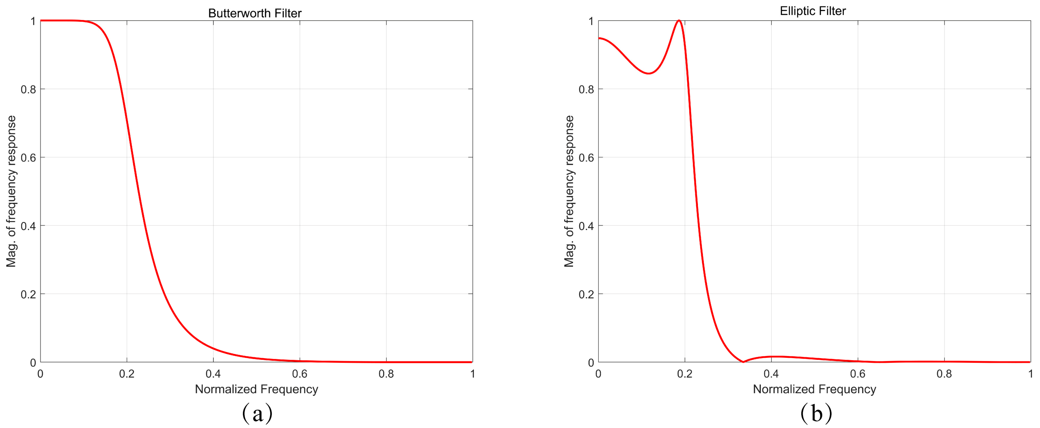
2.2. Filter Selection

2.2.1. Filter Introduction

The raw signal captured by the system exhibits considerable noise, so it is necessary to design a filter to remove noise for data processing.

As can be seen from Figure 2, the passband of the Butterworth filter is the flattest, and the stopband drops slowly. The elliptical filter is steeper than it and has a narrower transition bandwidth, but it fluctuates in both the passband and the stopband. Compared to other filter types such as elliptic filters, Butterworth filters have three balanced characteristics: linear phase response, flat band-response, and progressive attenuation [20]. These three characteristics make the Butterworth filter perform well in balancing signal fidelity, denoising effect, and implementation complexity, and they are suitable for most applications where smooth response and good signal quality are required.

Pre-filtering is applied to restrict the frequency range of the input signal, laying the groundwork for the subsequent classification model by achieving the following:

(1)

Reducing the number of IMFs: This helps eliminate unnecessary modes caused by high-frequency noise;

(2)

Enhancing computational efficiency: Since the computational complexity of EMD rises with signal complexity, pre-filtering alleviates the processing load for subsequent decomposition steps.

2.2.2. Filter Design

The first step is to determine the design parameters. Now, we need to determine the following key parameters [21]: (1) passband frequency ($W_p$); (2) stopband frequency ($W_s$); (3) maximum passband attenuation ($R_p$); (4) minimum stopband attenuation ($A_s$); and (5) sampling frequency ($F_s$). The initial parameter is set as $W_p=1 \mathrm{Hz}$; $W_s=10 \mathrm{Hz}$; $R_p=1 \mathrm{dB}$; $A_s=30 \mathrm{dB}$; $F_s=1000 \mathrm{Hz}$.

The subsequent phase involves determining the normalized frequency value. $f_p$ and $f_s$ denote the passband frequency and stopband frequency, respectively. The formula is as follows [22]:

$$W_p={\displaystyle \frac{f_p}{F_s/2}}$$

(1)

$$W_s={\displaystyle \frac{f_s}{F_s/2}}$$

(2)

The third phase entails calculating the order $N$ of the filter, and in order to ensure that the attenuation of the filter meets the requirements, we need to calculate the required order $N$.

$$N=\left[{\displaystyle \frac{\log \left(\frac{{10}^{\raisebox{1ex}{$A_s$}\!\left/ \!\raisebox{-1ex}{$10$}\right.}-1}{{10}^{\raisebox{1ex}{$R_p$}\!\left/ \!\raisebox{-1ex}{$10$}\right.}-1}\right)}{2\log \left(\frac{W_s}{W_p}\right)}}\right]$$

(3)

The fourth step is to calculate the cutoff frequency $W_c$. Once the order $N$ is known, the cutoff frequency $W_c$ can be calculated, serving as the cornerstone of the filter’s design. The subsequent formula determines the appropriate cutoff frequency based on the order of the filter and the passband attenuation.

$$W_c=W_p\times {\left({\displaystyle \frac{1}{{10}^{\raisebox{1ex}{$R_p$}\!\left/ \!\raisebox{-1ex}{$10$}\right.}-1}}\right)}^{{\displaystyle \frac{1}{2N}}}$$

(4)

The fifth step is to calculate the transfer function of the filter. For Butterworth filters, the transfer function in the analog domain takes the following form:

$$H(s)={\displaystyle \frac{1}{1+{(s/W_c)}^{2N}}}$$

(5)

The sixth step entails designing and implementing the digital filter by employing the bilinear transform to transition from the analog domain to the digital domain. This transformation process maps the analog frequency variable s to the digital frequency variable $z^{-1}$, where $F_s$ denotes the sampling frequency. By doing so, this method ensures that the frequency response characteristics of the filter are accurately preserved, thereby minimizing the risk of frequency distortion during the conversion.

$$s={\displaystyle \frac{2F_s}{1-z^{-1}}}\cdot {\displaystyle \frac{1+z^{-1}}{1-z^{-1}}}$$

(6)

By replacing s in the transfer function $H(s)$ of the analog filter with the expression after bilinear transformation, the response characteristic of the digital filter can be obtained.

Inside Figure 3, the blue line depicts the raw dynamic resistance signal captured throughout the welding procedure, which is contaminated with significant high-frequency noise. To address this, a Butterworth low-pass filter is employed to effectively smooth the signal and remove unwanted high-frequency components. And the resulting filtered signal is illustrated by the red line.

3. Signal Analysis

3.1. Welding Surface Image Analysis

Figure 4 illustrates the surface image of the actual occurrence of these welding defects; (a) shows the surface weld spot condition of a normally welded workpiece. The weld spot is complete and uniform, with a diameter and shape that meet expectations, exhibiting no obvious defects. The surface conditions of three welding defects differ markedly from normal welding (a). Weld spatter (b) includes internal spatter, occurring between material layers and detectable only via tensile testing, resembling normal weld surfaces. False welding (c) features a smaller weld spot diameter due to incomplete fusion, yielding insufficient strength and a less full appearance. Edge welding (d) produces an incomplete, irregularly shaped weld spot. Due to the welding position being close to the edge, metal may overflow, preventing the formation of a complete circular weld spot, with noticeable metal flow at the edge.

The surface solder joint image in Figure 4 can preliminarily observe the differences between normal welding, welding spatter, false welding, and edge welding, but the intrinsic quality and performance of the solder joint cannot be comprehensively evaluated by surface characteristics alone. Therefore, it is necessary to measure the tensile force of the solder joints by tensile experiments to further verify these differences and reveal the actual strength of the solder joints.

Figure 5 illustrates the schematic diagram of the tensile test. In this experiment, the weldment is securely fixed in the grips of the tensile testing machine. To prevent the weldment from slipping within the grips, pads are typically added to enhance the clamping effect, ensuring the stability of the specimen during the tensile process. Prior to conducting the tensile test, the tensile testing machine must be calibrated to guarantee the accuracy and reliability of the test data. Once calibration is complete, the tensile testing machine is activated, and the specimen is stretched at a uniform speed until the tensile force reaches its peak and then rapidly decreases, at which point the tensile process concludes.

As shown in

Table 2. Solder joint diameter and tensile force.

Weld Category	Solder Joint Diameter (mm)	Drawing Force (N)
Normal welding	6.792	5801.1
Welding spatter	6.503	5336.3
False welding	4.755	2517.4

, with identical parametric settings, the pull force of the spattered solder joint is lower than that of the normal solder joint. Under the condition of false welding, the diameter of the solder joint is significantly smaller than that of the normal solder joint, and its tensile force is below the minimum standard of 3080 N [23], which does not meet the requirements of the basic standard.

Surface image analysis shows that the solder joints of normal welding, welding spatter, and false welding are different in appearance, but for internal defects such as internal spatter, surface observation is difficult to provide sufficient information. Tensile experiments further verified these differences by tensile shear force; for example, the tensile shear force of false welding is significantly lower than that of normal welding, while the internal spatter shows only a slight decrease. Nevertheless, tensile test, as an afterthought test, cannot monitor the welding process in real time. Therefore, we introduced dynamic resistance curve analysis and explored a real-time classification method for solder joint quality by using the characteristics of resistance changes during welding so as to make up for the shortcomings of surface images and tensile experiments.

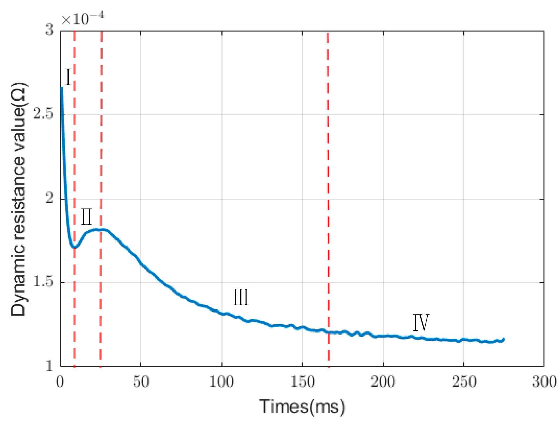
3.2. Dynamic Resistance Signal Curve

Dynamic resistance (DR) stands out as one of the most widely employed and effective process signals in the domain of RSW for the purpose of quality assessment and monitoring [24]. The interpretation of DR should take into account material characteristics, surface conditions, and process parameters. Correlating the DR signal with the physical phenomena of the welding process can clarify its physical significance for different metals at various stages, providing key insights for precise welding control and quality improvement. Quantitative models and co-simulations enhance signal interpretability and drive the shift from empirical control to physically driven intelligent monitoring [25]. The DR curve reflects the nugget size, spatter risk, and contact conditions through characteristic parameters. Combined with modeling and real-time monitoring, it provides a high-precision and low-cost quality evaluation and process optimization scheme for resistance spot welding. The reduction in resistance is strongly linked to the expansion of the contact area’s diameter but not the growth of the nugget [26]. Temperature and contact area analysis revealed resistance peak and drop mechanisms to support welding quality monitoring, especially for automated control and data-driven scenarios.

As depicted in Figure 6, the welding DR curve can be segmented into four distinct stages: the contact stage, the temperature melting stage, the nugget growth stage, and the cooling stabilization stage [27].

In phase I, the welding current passes through micro-contact points on the workpiece surface, creating a current concentration effect. Due to the high current density, the local temperature rises sharply, causing metal softening and an increase in contact area, which leads to a significant drop in DR. In phase II, as heat accumulates and as the temperature reaches the material’s melting point, the nugget begins to form. The resistivity increases slowly with the rising temperature, causing a gradual rise in dynamic resistance. In phase III, the nugget absorbs heat, and the welding center transitions into a liquid phase. The contact area diminishes, while the convective influence of the liquid phase further amplifies resistivity, leading to a sustained elevation in DR. In phase IV, the nugget size reaches its maximum and stabilizes, causing the DR to change very slowly, almost negligibly.

Taking into account potential welding imperfections encountered within the real-world production procedure, this research investigated three prevalent defects, namely welding spatter, false welding, and edge welding. The DR profile depicted in Figure 7 illustrates typical welding conditions alongside the other three weld imperfections. It can be observed that the DR curve changes significantly when there is a defect in the solder joint.

In the case of welding spatter, excessive welding current or improper pressure causes an overflow of molten metal at the welding center, leading to ejection and a significant reduction in contact area. As a result, the DR curve shows a notable decline in phase III. Even though spatter does not substantially diminish the mechanical strength of the weld joint, it weakens energy absorption capacity, causes energy waste, and accelerates electrode wear.

During edge welding, the DR curve is similar to that of normal welding, with a slow rise in phase II and a decline in phase III due to nugget formation. However, restricted by the edge effect, the nugget size is smaller and often accompanied by metal expulsion, shortening the duration of nugget expansion. This leads to a temporary peak appearing within the DR profile, with the overall peak duration being shorter than that of the spatter type. The nugget may not form sufficiently, resulting in solder joint strength below design requirements.

On the subject of false welding, the DR curve differs significantly from that of normal welding. While normal welding shows an upward trend in phase II, false welding exhibits a continuous decline or only a slight rise in phases II–III, with no distinct peak, indicating ineffective nugget formation. In this case, the solder joint easily falls off, or the mechanical strength is insufficient when subjected to external force.

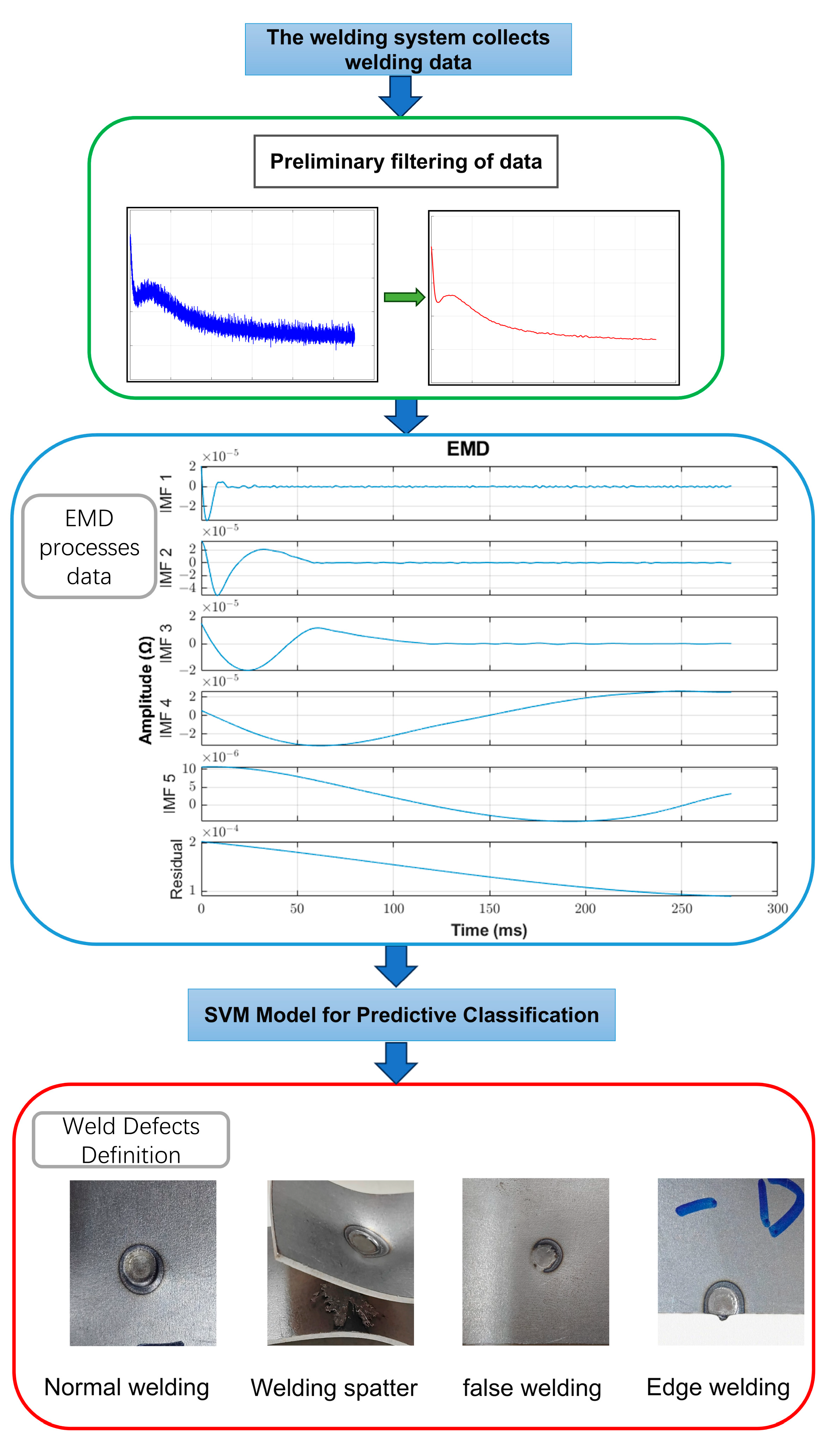
3.3. Empirical Mode Decomposition (EMD) of Welding Dynamic Resistance Signals

Within the domain of contemporary signal processing techniques, EMD is a powerful data processing tool, especially for the analysis of nonlinear and non-stationary data. The EMD methodology, introduced by Huang et al. [28], is capable of decomposing complex signals into a series of IMFs, which are the fundamental oscillating patterns of the signal and reveal the intrinsic characteristics of the data. The EMD processing steps for DR signal characteristics of resistance welding are as follows [29]:

(1)

Assuming that the dynamic resistance signal is $x\left(t\right)$, take the sequence $m\left(t\right)$, composed of the upper and lower envelope local means;

(2)

Let $h_1\left(t\right)=x\left(t\right)-m\left(t\right)$, provided $h_1\left(t\right)$ meets the IMF requirement; then, it is the first IMF component. On the contrary, $h_1\left(t\right)$ serves as the initial dataset for reiterating the procedures outlined in steps (1) and (2) for j times to obtain $h_{1j}\left(t\right)=h_{1(j-1)}\left(t\right)-m_{1j}\left(t\right)$ so that $h_{1j}\left(t\right)$ meets the IMF conditions to derive the first IMF, which is marked as $c_1(t)=h_{1j}\left(t\right)$;

(3)

Subtract $c_1\left(t\right)$ from $x\left(t\right)$ to obtain the following residual:

$$r_1\left(t\right)=x\left(t\right)-c_1\left(t\right)$$

(7)

Repeat the above steps with $r_1\left(t\right)$ as the original data to obtain the second IMF $c_2\left(t\right)$ of $x\left(t\right)$. Similarly, once $r_n\left(t\right)$ exhibits monotonic behavior and ceases to yield IMF constituents, the cycle ends, and $n$ IMF components are obtained. The final dynamic resistance signal $x\left(t\right)$ is broken down into the summation of $n$ IMF components plus a single residual term:

$$x\left(t\right)={\displaystyle \sum _{i=1}^n{c}_i\left(t\right)+r_n\left(t\right)}$$

(8)

IMFs are selected based on energy contribution exceeding 80% and Spearman correlation with defect labels above 0.4, ensuring an orthogonality index (OI) below 0.1 to effectively separate independent frequency components of Q235 spot welding signals. Redundant IMFs are filtered using an energy threshold of 5% and by excluding IMFs with pairwise correlations greater than 0.4. The three selected IMFs were optimized to ensure effective differentiation of Q235 spot welding defects, including normal, spatter, false welding, and edge welding.

On the basis of the basic principle and decomposition process of EMD algorithm, this paper further applies it to real signal data processing and compares and analyzes it with the wavelet packet decomposition (WPD) algorithm. Compared to WPD, EMD demonstrates a superior ability to efficiently decompose complex signals and retain critical information to provide more accurate and reliable features for subsequent classification models to improve training and prediction performance. The decomposition process of EMD adaptively divides the signal into different IMFs according to the intrinsic properties of the signal itself, which is particularly suitable for the nonlinear and time-varying characteristics of the welding signal. In contrast, the WPD method relies on pre-set decomposition levels and basic functions, and its inherent rigid framework is difficult to fully adapt to the multi-scale dynamic characteristics of complex signals, thus limiting its application effect and applicability in welding defect detection.

4. Solder Joint Quality Prediction Based on EMD-SVM

4.1. Support Vector Machine

A comprehensive overview of SVM is provided in references [30,31], while a concise summary is presented here. The primary goal of SVM is to perform classification by identifying an optimal hyperplane that cleanly divides data into separate categories with the maximum margin. SVM achieves this by maximizing the margin between the hyperplane and the closest data points on either side, thus identifying the most effective hyperplane that separates the data in the high-dimensional feature space. This maximum margin strategy enhances the model’s generalization capability. For data that are not linearly separable, SVM leverages kernel functions to map the data into a higher-dimensional Hilbert space, facilitating the identification of hyperplanes that can effectively separate the data in this expanded feature space.

Given an available training dataset denoted as ${\{(x_i,y_i)\}}_{i=1}^l$, where $x_i\in R^n$ is the feature vector and $y_i\in \{-1,1\}$ is the corresponding classification label, SVM finds the optimal hyperplane $(w,b)$ that maximizes the margin between classes. The original optimization problem of SVM is as follows:

$${\min }_{w,b,\xi }{\displaystyle \frac{1}{2}}\Vert w{\Vert }^2+C{\displaystyle \sum _{i=1}^l({\xi }_i+{\xi }_i^{*})}$$

(9)

The constraints are as follows:

$$\left\{\begin{array}{l}{y}_i(w^T\varphi (x_i)+b)\ge 1-{\xi }_i\\ {\xi }_i\ge 0,\hspace{1em}\forall i=1,\dots ,l\end{array}\right.$$

The normal vector $w$ determines the direction of the hyperplane. b is the bias. $C>0$ is the penalty coefficient that balances the classification margin and misclassified points, and the variable ${\xi }_i$ serves as the slack variable, quantifying the permissible extent of misclassification within the optimization framework.

Through the incorporation of Lagrange multipliers ${\alpha }_i$ and ${\eta }_i$, the aforementioned optimization problem can be reformulated into its corresponding dual representation, facilitating a more tractable solution.

$${\min }_{\alpha }D(\alpha )={\displaystyle \sum _{i=1}^l{\alpha }_i}-{\displaystyle \frac{1}{2}}{\displaystyle \sum _{i=1}^l{\displaystyle \sum _{m=1}^l{\alpha }_i}}{\alpha }_m{y}_i{y}_{m}K(x_i,x_m)$$

(10)

The constraints are as follows:

$$\left\{\begin{array}{l}0\le {\alpha }_i\le C,\hspace{1em}\forall i=1,\dots ,l\\ {\displaystyle \sum _{i=1}^l{\alpha }_i}{y}_i=0\end{array}\right.$$

where $K(x_i,x_m)$ is defined as the kernel function and is used to compute the scalar product of the sample points in the input space. SVM can avoid the explicit calculation of high-dimensional maps by kernel function and then search for linearly separable hyperplanes.

Selecting an appropriate kernel function is essential for optimizing the performance of support vector machines. Various kernel functions are better suited to different tasks and data distributions, so the choice of the most suitable kernel function must be determined by the specific characteristics of the problem.

In this paper, the problem of welding defect signal classification is usually characterized by highly nonlinear distribution characteristics and complex classification boundaries. Therefore, it is particularly important to select kernel functions with strong nonlinear mapping ability and strong generality. In this case, the radial basis function (RBF) kernel function can effectively deal with the nonlinear characteristics of the data and improve the classification performance. The RBF kernel function is $K(x_i,x_m)=\exp (-\gamma \Vert x_i-x_m{\Vert }^2)$. After the optimization is completed by introducing Lagrange multipliers, the classification decision function at the end can be formulated as follows:

$$f(x)=\mathrm{sign}\left({\displaystyle \sum _{i=1}^n{\alpha }_i}{y}_i\exp \left(-{\displaystyle \frac{\left|\right|x_i-x|{|}^2}{2{\sigma }^2}}\right)+b\right)$$

(11)

where the support vector corresponds to ${\alpha }_i>0$. These support vectors define the optimal hyperplane and have high interpretability.

In this study, we initially set the penalty parameter $C=10$ and the kernel parameter $\gamma =0.01$ for the SVM.

SVM is a supervised learning algorithm based on maximum interval classification, which has a solid theoretical foundation and excellent application performance. With the rise of deep learning, the application of SVM has decreased in some fields, but its advantages in small samples, high-dimensional data, and non-linear classification problems make it still one of the important algorithms within the domain of machine learning.

4.2. The Overall Model of EMD-SVM Was Used to Evaluate Solder Joint Quality

An SVM classification framework leveraging EMD is herein introduced, enabling the assessment of RSW quality. The complete procedure is illustrated in Figure 8. The algorithm presented herein is segmented into the subsequent three phases:

(1)

In accordance with the surface phenomena of RSW, four types of welding were defined: normal welding, welding spatter, false welding, and edge welding. Among them, level 1 is normal welding, level 2 is welding spatter, level 3 is false welding, and level 4 is edge welding. The DR data after integration processing were taken as the dataset;

(2)

The filtered DR data were decomposed through EMD to yield several modal components with varying properties, including IMFs components and residuals;

(3)

A classification model using SVM was established to predict solder joint quality types, utilizing the original signal, IMFs components, and residual components of the four visual features as input data.

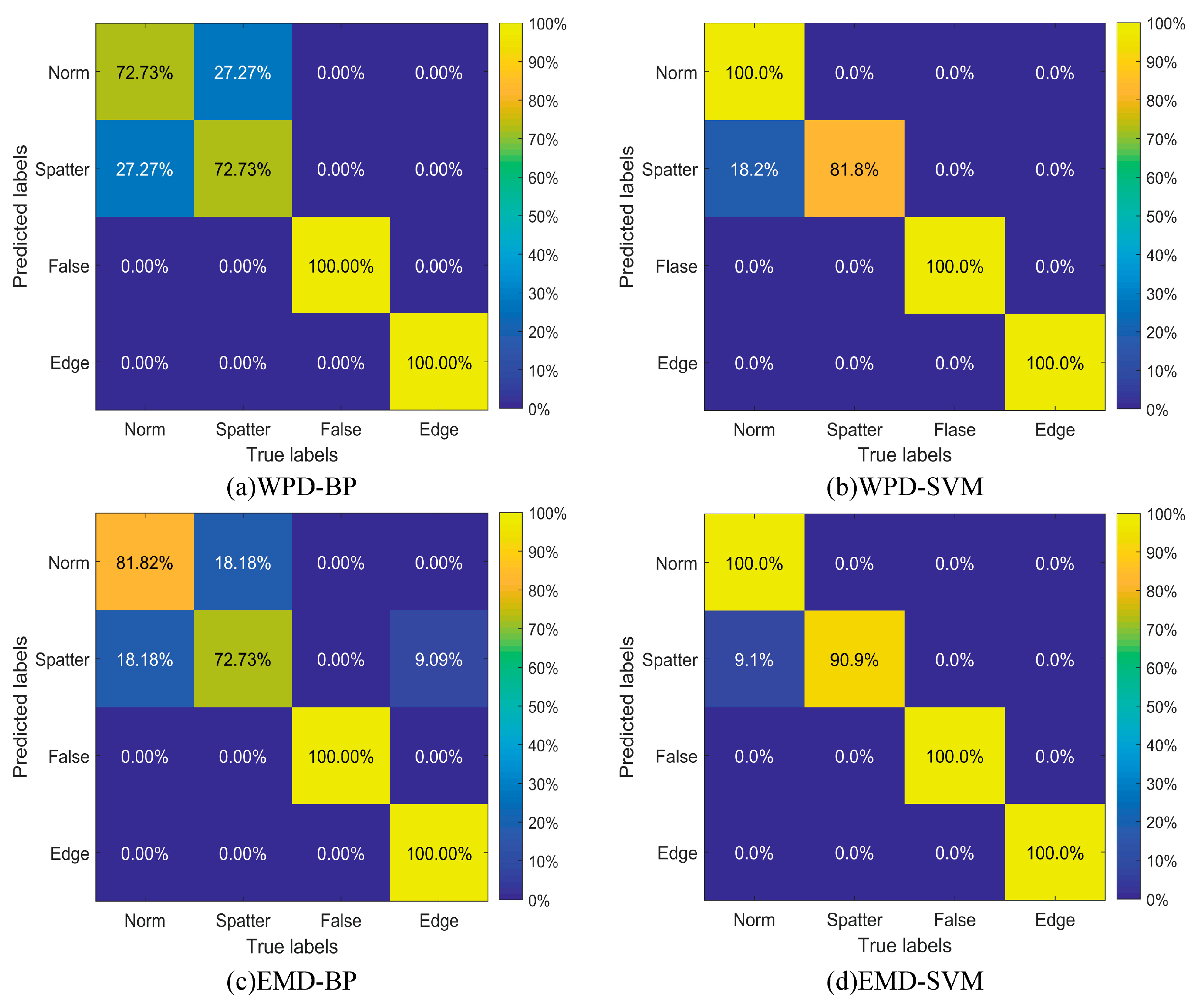
4.3. Results and Discussion

From 144 samples collected to normal welding, welding spatter, false welding, and edge welding, 100 DR data were taken as training samples, and 44 DR data were employed as test samples. Subsequent to EMD treatment, the training samples underwent random cleaning, where 70% were assigned to the training set and 30% to the validation set. The analysis and prediction algorithms were implemented using MATLAB software (matlab R2021b). In this study, EMD-SVM was employed to predict solder joint quality types, with a backpropagation (BP) neural network used for comparison and analysis of the prediction results. To highlight the advantages of EMD, the WPD method was contrasted with the EMD approach.

In this work, five classification algorithms: BP, SVM, WPD-BP, WPD-SVM, and EMD-BP, are proposed, and the classification performance of the designed mixed model of EMD-SVM is systematically compared. Different parameters of the model will have different effects on the results of the actual classification problem, which are mainly determined by the correlation between features, the number of categories, the volume of the input data, and the sample count. In the procedure of parameter adjustment and optimization, the kernel function of the SVM classifier demonstrates strong predictive capability and guarantees prediction impartiality. These comparative experiments solely modified the central component of the algorithm, while the configurations of other unrelated parameters were kept constant.

The BP neural network consists of three distinct layers. The quantity of neurons in the input layer amounts to 12, corresponding to the number of input features as shown in

Table 3. The characteristic indexes of the target signal.

Features	Equation	Description
$r_{mean}$	$r_{mean}={\displaystyle \sum _{i=1}^n{r}_i}/n$	The average value of the whole signal; n is the signal length
$\sigma$	$\sigma =\sqrt{{\displaystyle \frac{1}{n}}{\displaystyle \sum _{i=1}^n{(r_i-r_{mean})}^2}}$	The standard deviation value of the signal
$r_{\max }$	-	The maximum amplitude value in the signal
$r_{\min }$	-	The minimum amplitude value in the signal
$r_{mid}$	$r_{mid}={\displaystyle \frac{r_{\max }+r_{\min }}{2}}$	The average value of the maximum resistance and minimum resistance value
$S$	$S={\displaystyle \frac{n}{(n-1)(n-2)}}{\displaystyle \sum _{i=1}^n{\left(\frac{r_i-r_{mean}}{\sigma }\right)}^3}$	Measures asymmetry of the signal distribution
$K$	$K={\displaystyle \frac{n}{(n-1)(n-2)}}{\displaystyle \sum _{i=1}^n{\left(\frac{r_i-r_{mean}}{\sigma }\right)}^4}-3$	Measures the “tailedness” or sharpness of the signal distribution.
$\Delta$	$\Delta =r_{\max }-r_{\min }$	The range value between the maximum point and the minimum point in the signal
$C_F$	$C_F=\max (|r_i|)/\sqrt{{\displaystyle \frac{1}{n}}{\displaystyle \sum r_i^2}}$	The ratio of the peak value of the signal to the root mean square value, indicating signal spikes.
$N_P$	$N_P={\displaystyle \sum _{i=2}^{n-1}\mathbb{I}}(r_i>r_{i\pm 1} )$	The count of local peaks in the signal; $\mathbb{I}$ is indicator function
$R_P$	$R_P={\displaystyle \frac{N_P}{(n-1)T}}$	The rate at which peaks occur in the signal;$T$ is the sampling interval.
$r_{ZCR}$	$r_{ZCR}={\displaystyle \frac{1}{(n-1)T}}{\displaystyle \sum _{i=1}^{n-1}\mathbb{I}}(r_i\cdot r_{i+1}<0)$	The frequency of signal amplitude sign changes (zero-crossings) per unit time/length

, and the input feature is the feature value extracted from the DR value obtained by calculating the ratio of the collected voltage to the current and then filtering, including mean, kurtosis, etc. The quantity of neurons in the output layer amounts to four, matching the total count of solder joint quality categories, with each neuron indicating the classification likelihood for the associated weld category. The quantity of neurons in the intermediate layer was set to 10. The initial and intermediate transfer functions are Tansig functions, whereas the final transfer functions are Softmax functions tailored for multi-classification tasks. The training function is the Levenberg–Marquardt algorithm, which is especially suitable for small- or medium-sized networks. To guarantee that the outcomes of the neural network training procedure remained uniform across each execution of the program, the random number seed was set to 70 within the software. The training duration, training objective, and learning rate of the BP network were established at 500, 0.02, and 0.01, respectively.

When designating “normal welding” as the positive class, these measures were operationalized as follows: TP (true positives) constitutes correctly identified normal welding specimens; TN (true negatives) reflects non-positive cases appropriately excluded from this classification; FP (false positives) represents erroneous assignments of atypical welds to the normal category; FN (false negatives) captures undetected normal welding misclassified as defective types. A consistent analytical protocol was systematically implemented across all defect classifications through permutation of positive class designation in corresponding confusion matrices, maintaining methodological parity in multi-category evaluation.

The detailed outcomes of BD, WPD-BP, EMD-BP, SVM, WPD-SVM, and EMD-SVM are presented in

Table 4. Comparative assessment of performance outcomes across various models.

Model	Training Time (s)	Accuracy of Train Set (%)	Accuracy of Test Set (%)	Significance (p < 0.05)
BP	0.18	80.81	84.09	0.001
SVM	0.09	90.00	90.91	0.018
WPD-BP	0.16	82.26	86.36	0.001
WPD-SVM	0.12	95.60	95.45	0.045
EMD-BP	0.15	89.36	88.64	0.002
EMD-SVM	0.11	96.88	97.73	-

. The accuracy of the proposed EMD-SVM framework (97.73% accuracy) was higher than that of EMD-BP (88.64% accuracy) and superior to the fundamental BP framework (84.09% accuracy) and SVM (90.91% accuracy). Through comparative analysis, it became obvious that whether the SVM model or BP model, the performance of signals processed based on EMD in defect detection was significantly better than that processed by WPD. As a result, the signals processed by EMD showed higher accuracy in the classification task, significantly enhancing the effectiveness of the model. This study employed 10-fold cross-validation to investigate whether overfitting occurred due to a small sample size. The “training set accuracy” reported in Table 4 represents the average accuracy across the training sets during the 10-fold cross-validation process. The results indicate that the training set accuracy was not significantly higher than the test set accuracy, suggesting that overfitting is not present. The EMD-SVM approach exhibited the greatest classification precision and effectiveness compared to other models.

Furthermore, Figure 9 shows the confusion matrices of the four classification approaches contrasted. Within a matrix, the rows indicate the forecasted categories, while the columns denote the true categories. The results show that the classification performance of class 1 (normal solder joints) and class 2 (welding spatter solder joints) was generally poor in all models, which may be due to the highly similar distribution of the two types of solder joints in the time-frequency domain feature space. It is noteworthy that the EMD-SVM hybrid approach had the best performance in inter-class discrimination ability, and its classification accuracy was improved by 2.28% compared with the baseline model. This improvement is mainly due to the time-frequency decoupling ability of EMD algorithm to non-stationary signals, and the reconstruction of IMFs effectively filters out high-order dynamic interference during welding spatter process while combining with the separability of SVM kernel space-mapping optimization features, thus significantly enhancing the clarity of inter-class decision boundaries.

Among the algorithms evaluated in this paper, the integration of SVM and EMD yields the most optimal performance. The experimental results show that the EMD-SVM model has significant application potential in welding quality monitoring and defect detection, especially in complex signal analysis and real-time monitoring scenarios, which can better support the accurate identification of defects.

5. Conclusions

Drawing on the evaluation and comparative assessment of DR signals, this study introduces a specialized approach for extracting characteristic signal values to enable online detection of RSW defects, subsequently validating the approach and presenting the subsequent findings:

• A high-accuracy online monitoring framework for welding current and voltage signals was developed to deliver comprehensive data for the quality assessment of RSW on Q235 mild steel;
• The experiment reveals that notable distinctions exist between the DR profiles of normal welding and defective welding, with clear variations also present among various defect categories. The DR of welding spatter will decrease instantaneously in phase III. The DR of the false welding lacks the characteristics of nugget formation in phase II. The phase III of edge welding concludes earlier than normal welding, and the DR signal drops instantaneously due to the production of the discharge;
• This study investigated main defects in the RSW process (welding spatter, false welding, and edge welding) and extracted 12 features of normal and defective joints using a Butterworth filter. A new EMD-SVM classification method is proposed to improve the accuracy of distinguishing normal from spatter welding points. Through an online quality evaluation of 144 welding points, the method achieved 97.73% classification accuracy, outperforming other models. An online quality evaluation and defect classification model was developed, enabling rapid and accurate classification of welding points.

References

1. Wang, L.; Hou, Y.; Zhang, H.; Zhao, J.; Xi, T.; Qi, X.; Li, Y. A New Measurement Method for the Dynamic Resistance Signal during the Resistance Spot Welding Process. Meas. Sci. Technol. 2016, 27, 95009. [Google Scholar] [CrossRef]
2. Zhao, D.; Vdonin, N.; Slobodyan, M.; Butsykin, S.; Kiselev, A.; Gordynets, A.; Wang, Y. Dynamic Resistance Signal-Based Wear Monitoring of Resistance Spot Welding Electrodes. Int. J. Adv. Manuf. Technol. 2024, 133, 3267–3281. [Google Scholar] [CrossRef]
3. Meilinger, Á.; Kovács, P.Z.; Lukács, J. High-Cycle Fatigue Characteristics of Aluminum/Steel Clinched and Resistance-Spot-Welded Joints Based on Failure Modes. Metals 2024, 14, 1375. [Google Scholar] [CrossRef]
4. Zhao, D.; Bezgans, Y.; Wang, Y.; Du, W.; Vdonin, N. Research on the Correlation between Dynamic Resistance and Quality Estimation of Resistance Spot Welding. Measurement 2021, 168, 108299. [Google Scholar] [CrossRef]
5. Stavropoulos, P.; Sabatakakis, K. Quality Assurance in Resistance Spot Welding: State of Practice, State of the Art, and Prospects. Metals 2024, 14, 185. [Google Scholar] [CrossRef]
6. Gao, X.; Wang, Y.; Chen, Z.; Ma, B.; Zhang, Y. Analysis of Welding Process Stability and Weld Quality by Droplet Transfer and Explosion in MAG-Laser Hybrid Welding Process. J. Manuf. Process. 2018, 32, 522–529. [Google Scholar] [CrossRef]
7. Wang, C.; Wang, C.; Gao, X.; Tian, M.; Zhang, Y. Research on Microstructure Characteristics of Welded Joint by Magneto-Optical Imaging Method. Metals 2022, 12, 258. [Google Scholar] [CrossRef]
8. Peng, P.; Fan, K.; Fan, X.; Zhou, H.; Guo, Z. Real-Time Defect Detection Scheme Based on Deep Learning for Laser Welding System. IEEE Sens. J. 2023, 23, 17301–17309. [Google Scholar] [CrossRef]
9. Guo, S.; Wang, D.; Chen, J.; Feng, Z.; Guo, W. Predicting Nugget Size of Resistance Spot Welds Using Infrared Thermal Videos With Image Segmentation and Convolutional Neural Network. J. Manuf. Sci. Eng. 2021, 144, 021009. [Google Scholar] [CrossRef]
10. Zhou, L.; Zhang, R.X.; Yang, H.F.; Huang, Y.X.; Song, X.G. Microstructure and Mechanical Properties of Friction Stir Welded Q235 Low-Carbon Steel. J. Mater. Eng. Perform. 2018, 27, 6709–6718. [Google Scholar] [CrossRef]
11. Chen, S.; Sun, T.; Jiang, A.; Qi, J.; Zeng, R. Online Monitoring and Evaluation of the Weld Quality of Resistance Spot Welded Titanium Alloy. J. Manuf. Process. 2016, 23, 183–191. [Google Scholar] [CrossRef]
12. Chen, S.; Wu, N.; Xiao, J.; Li, T.; Lu, Z. Expulsion Identification in Resistance Spot Welding by Electrode Force Sensing Based on Wavelet Decomposition with Multi-Indexes and BP Neural Networks. Appl. Sci. 2019, 9, 4028. [Google Scholar] [CrossRef]
13. Zhao, D.; Wang, Y.; Liang, D.; Ivanov, M. Performances of Regression Model and Artificial Neural Network in Monitoring Welding Quality Based on Power Signal. J. Mater. Res. Technol. 2020, 9, 1231–1240. [Google Scholar] [CrossRef]
14. Peng, S.; Sun, S.; Yao, Y.-D. A Survey of Modulation Classification Using Deep Learning: Signal Representation and Data Preprocessing. IEEE Trans. Neural Netw. Learn. Syst. 2022, 33, 7020–7038. [Google Scholar] [CrossRef] [PubMed]
15. Abate, F.; Huang, V.K.L.; Monte, G.; Paciello, V.; Pietrosanto, A. A Comparison between Sensor Signal Preprocessing Techniques. IEEE Sens. J. 2015, 15, 2479–2487. [Google Scholar] [CrossRef]
16. Voznesensky, A.; Kaplun, D. Adaptive Signal Processing Algorithms Based on EMD and ITD. IEEE Access 2019, 7, 171313–171321. [Google Scholar] [CrossRef]
17. Fan, X.; Gao, X.; Zhang, N.; Ye, G.; Liu, G.; Zhang, Y. Monitoring of 304 Austenitic Stainless-Steel Laser-MIG Hybrid Welding Process Based on EMD-SVM. J. Manuf. Process. 2022, 73, 736–747. [Google Scholar] [CrossRef]
18. Li, W.; Cerjanec, D.; Grzadzinski, G.A. A Comparative Study of Single-Phase AC and Multiphase DC Resistance Spot Welding. J. Manuf. Sci. Eng. 2004, 127, 583–589. [Google Scholar] [CrossRef]
19. Samimi, M.H.; Mahari, A.; Farahnakian, M.A.; Mohseni, H. The Rogowski Coil Principles and Applications: A Review. IEEE Sens. J. 2015, 15, 651–658. [Google Scholar] [CrossRef]
20. Hussin, S.F.; Birasamy, G.; Hamid, Z. Design of Butterworth Band-Pass Filter. Politek. Kolej Komuniti J. Eng. Technol. 2016, 1, 32–46. [Google Scholar]
21. Lv, Z.; Gao, X.; Xiao, H.; Gao, P. Resistance Spot Welding Defect Detection Based on Vectorized Dynamic Resistance Signal and LightGBM Classifier. Meas. Sci. Technol. 2024, 35, 086113. [Google Scholar] [CrossRef]
22. Chen, D.; Yang, W.; Pan, M. The Dynamic Response of a Butterworth Low-Pass Filter in an Ac-Based Electrical Capacitance Tomography System. Meas. Sci. Technol. 2010, 21, 105505. [Google Scholar] [CrossRef]
23. JISZ3140:2017 Method of Inspection and Acceptance Levels for Resistance Spot Welds. Available online: https://kikakurui.com/z3/Z3140-2017-01.html (accessed on 25 April 2025).
24. Zhou, K.; Yao, P. Overview of Recent Advances of Process Analysis and Quality Control in Resistance Spot Welding. Mech. Syst. Signal Process. 2019, 124, 170–198. [Google Scholar] [CrossRef]
25. Xia, Y.-J.; Lv, T.; Ghassemi-Armaki, H.; Li, Y.; Carlson, B. Quantitative Interpretation of Dynamic Resistance Signal in Resistance Spot Welding. Weld. J. 2023, 102, 69s–87s. [Google Scholar] [CrossRef]
26. Tan, W.; Zhou, Y.; Kerr, H.W.; Lawson, S. A Study of Dynamic Resistance during Small Scale Resistance Spot Welding of Thin Ni Sheets. J. Phys. D Appl. Phys. 2004, 37, 1998–2008. [Google Scholar] [CrossRef]
27. Xing, B.; Xiao, Y.; Qin, Q.H.; Cui, H. Quality Assessment of Resistance Spot Welding Process Based on Dynamic Resistance Signal and Random Forest Based. Int. J. Adv. Manuf. Technol. 2018, 94, 327–339. [Google Scholar] [CrossRef]
28. Huang, N.E.; Shen, Z.; Long, S.R.; Wu, M.C.; Shih, H.H.; Zheng, Q.; Yen, N.-C.; Tung, C.C.; Liu, H.H. The Empirical Mode Decomposition and the Hilbert Spectrum for Nonlinear and Non-Stationary Time Series Analysis. Proc. R. Soc. Lond. A Math. Phys. Eng. Sci. 1998, 454, 903–995. [Google Scholar] [CrossRef]
29. Ge, H.; Chen, G.; Yu, H.; Chen, H.; An, F. Theoretical Analysis of Empirical Mode Decomposition. Symmetry 2018, 10, 623. [Google Scholar] [CrossRef]
30. Cortes, C.; Vapnik, V. Support-Vector Networks. Mach. Learn. 1995, 20, 273–297. [Google Scholar] [CrossRef]
31. Burges, C.J.C. A Tutorial on Support Vector Machines for Pattern Recognition. Data Min. Knowl. Discov. 1998, 2, 121–167. [Google Scholar] [CrossRef]
Figure 1. Resistance welding experimental system platform. (a) Welding robots; (b) MFDC spot welding gun; (c) voltage sensor; (d) electric current sensor; (e) data acquisition card; (f) control cabinet.
Metals 15 00504 g001
Figure 2. Filter comparison chart. (a) Butterworth filters; (b) elliptic filters.
Metals 15 00504 g002
Figure 3. Comparison between the raw signal and the filtered signal.
Metals 15 00504 g003
Figure 4. Image of defect surface in the experiment. (a) Normal welding; (b) spatter welding; (c) false welding; (d) edge welding (1-D numbering).
Metals 15 00504 g004
Figure 5. Schematic diagram of the tensile test for welded workpieces.
Metals 15 00504 g005
Figure 6. Dynamic resistance profile of Q235 mild steel resistance spot welding. (Ⅰ) the contact stage; (Ⅱ) the temperature melting stage; (Ⅲ) the nugget growth stage; (Ⅳ) the cooling stabilization stage.
Metals 15 00504 g006
Figure 7. Dynamic resistance profiles of various weld imperfections in the experiment.
Metals 15 00504 g007
Figure 8. Flowchart of the proposed resistance welding defect diagnosis method.
Metals 15 00504 g008
Figure 9. Comparison of the confusion matrix of four models.
Metals 15 00504 g009