A Feature Extraction Algorithm for Corner Cracks in Slabs Based on Multi-Scale Adaptive Gradient Descent

Abstract

Cracks at the corners of casting billets have a small morphology and rough surfaces. Corner cracks are generally irregular, with a depth of about 0.2–5 mm and a width of about 0.5–3 mm. It is difficult to detect the depth of cracks and the three-dimensional morphological characteristics. The severity of cracks is hard to evaluate with traditional inspection methods. To effectively extract the topographic features of corner cracks, a multi-scale surface crack feature extraction algorithm, based on weighted adaptive gradient descent, was proposed. Firstly, the point cloud data of the corners of the billet were collected by the three-dimensional visual inspection platform. The point cloud neighborhood density was calculated using the k-nearest neighbor method; then the weighted covariance matrix was used to calculate the normal rate of change. Secondly, the adaptive attenuation rate, based on normal change, was fused with the density weight, which can calculate the Gaussian weight in regard to the neighborhood. Gaussian weights were used to obtain the gradient changes between point clouds to acquire the multi-scale morphological features of the crack. Finally, the interference caused by surface and boundary effects was eliminated by DBSCAN density clustering. The complete three-dimensional morphology characteristics of the crack were obtained. The experimental results reveal that the precision rate, recall rate, and F-value of the improved algorithm are 96.68%, 91.32%, and 93.92%, respectively, which are superior to the results from the RANSAC and other mainstream algorithms. The three-dimensional morphological characteristics of corner cracks can be effectively extracted using the improved algorithm, which provides a basis for judging the severity of the defect.

1. Introduction

During the process of continuous casting production, the corners of casting billets are prone to small transverse cracks due to the influence of process factors, such as molten steel composition, mold taper, protective slag performance, and secondary cooling water distribution [1,2,3]. Corner cracks are highly prone to expansion during the rolling process, leading to serious edge crack defects in the steel strip, which degrades product quality and reduces the rolling efficiency [4,5,6,7].

Currently, corner crack detection for casting billets is mainly carried out through random inspections. Corner samples, approximately 100 mm in length and 30 mm in height, are cut from the billet corner. Samples need to be pickled on site for about 20 min to remove the iron oxide scale on the surface of the casting billet. After rinsing and air drying at a temperature lower than 40 °C, the sample is either manually inspected or photographed and the images uploaded to the quality control department to assess the severity of the surface defects. The entire process takes about 40 min. For relatively rough casting surfaces, it is particularly difficult to detect the crack detail characteristics and acquire crack depth information.

Traditional manual inspection and two-dimensional (2D) image inspection technologies are insufficient in terms of providing adequate information on the three-dimensional (3D) defect features of cracks to ensure accurate identification. Therefore, 3D visual inspection technology for the detection of corner crack defects in casting billets can obtain the 3D morphological characteristics of the defect area, assist the quality inspection department to analyze and grade the severity of the defect, and effectively improve the detection efficiency in terms of the defect [8,9].

At present, 3D defect detection technology relies on a laser displacement sensor to obtain the 3D contour point cloud data of the measured object. As a collection of 3D coordinate points, the point cloud can achieve fast and accurate non-contact detection of defects on the surface of an object by extracting the normal vector, curvature, and other characteristics of the point cloud data. Defect detection algorithms based on 3D point clouds can be classified into the following methods: (1) deep learning-based methods, with typical approaches including PointNet [10] and PointNet++ [11] for point cloud segmentation to obtain the features of the point cloud. Xu et al. [12] constructed the GDNet geometric inspection attention network, using a geometric decoupling module and a sharp–gradual module to segment point cloud features. Ma et al. [13] adopted a lightweight geometric affine module to build a pure residual PointNetMLP network to accelerate the training speed of the network model. Zhou et al. [14] utilized a feature embedding module, an attention module, and a classification module to form the TransPCNet network for sewer defect detection. Hu et al. [15] constructed a dual-stream region attention network by directly focusing on the region of interest through backpropagation to detect tiny defects in PCB board point clouds. The disadvantage of this method is that it requires a large amount of data for training, which means that it is difficult to process fine local features and has poor real-time performance. (2) Model registration-based methods: These methods register the point cloud to be inspected according to known model data. By comparing the differences between them, the location of the defect is obtained. Zeng et al. [16] used Iterative Closest Point (ICP) registration and nearest neighbor search methods for rail wear measurement. Cai et al. [17] employed neighborhood point feature segmentation for engine blade damage detection. Yang et al. [18] applied an over-constraint registration method for complex part milling and robot workpiece recognition. Wu et al. [19] located fine cracks through the use of regional reconstruction and partial point cloud registration. However, the drawback of these methods is that they need data from known models, which are relatively limited. (3) Model-free detection methods. Zhang et al. [20] used the Random Sample Consistency (RANSAC) algorithm to fit planes and segment weld point clouds for weld defect detection. Yang et al. [21] employed the RANSAC algorithm for the extraction and path planning of 3D welds of arc welding robots. These methods perform well on smooth surfaces, but struggle to handle complex geometries. Ma et al. [22] applied Principal Component Analysis (PCA) for feature extraction from discrete point clouds. Wu et al. [23] performed feature extraction on pit point clouds through the use of normal vector region clustering segmentation. Yu et al. [24] identified the 3D feature points through the curvature values, and the detection process was found to be inefficient, with room for improvement in regard to accuracy. Luo et al. [25] achieved indoor 3D point cloud plane segmentation through the use of region growing, with constraints. Li et al. [26] combined the RANSAC algorithm with 2D image algorithms to achieve object detection, using LiDAR technology, with high detection accuracy, but there is still room for improvement.

For the detection of objects with a flat surface, 3D visual inspection equipment can collect the point cloud data of the crack area with a coherent overall morphology and complete boundary area, which can be used to effectively extract the characteristics of the crack. Due to the irregularity and uneven rust on the surface of casting billets, there is a lack of point-to-point connection information and geometric structures between any of the point cloud data and its neighborhood points. It is difficult to effectively obtain the boundary and topographic features of point clouds when extracting them. The RANSAC algorithm cannot solve the problem of pseudo-planar and non-planar networks. The density clustering method utilizes the density difference between cracked point clouds and non-cracked point clouds to complete the clustering process, but it cannot resolve the issues related to missing information in terms of clustering at the edges. Methods based on curvature and normal vectors fail to extract defect features when the crack surface is relatively flat or steep.

Gradient sensitivity is utilized in regard to surface variations for defect detection, which can effectively compensate for the shortcomings of classical algorithms. Deng et al. [27] used morphological gradients to segment point cloud data, with an error of less than 0.1 mm. Chen et al. [28] proposed a gradient clustering-based edge optimization extraction algorithm to effectively eliminate edge misdetections. Zhang [29] et al. applied quantitative field gradients for the automatic extraction of step lines in open-pit mine point clouds, with an error rate of less than 10%. However, for the detection of cracks on complex steel surfaces, the existing studies could not effectively extract defect features. Under the condition that a relatively complete point cloud dataset can be obtained, a multi-scale steel surface crack feature extraction method, based on adaptive gradient descent, was proposed.

2. Related Work

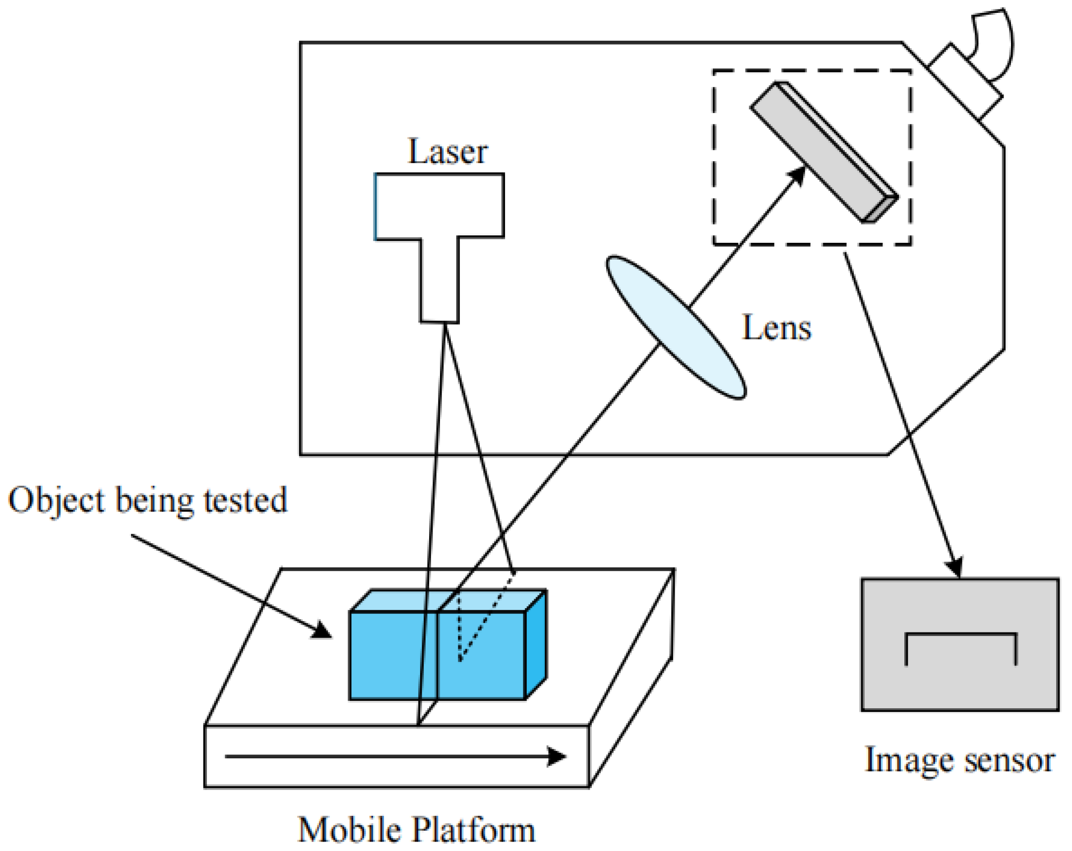
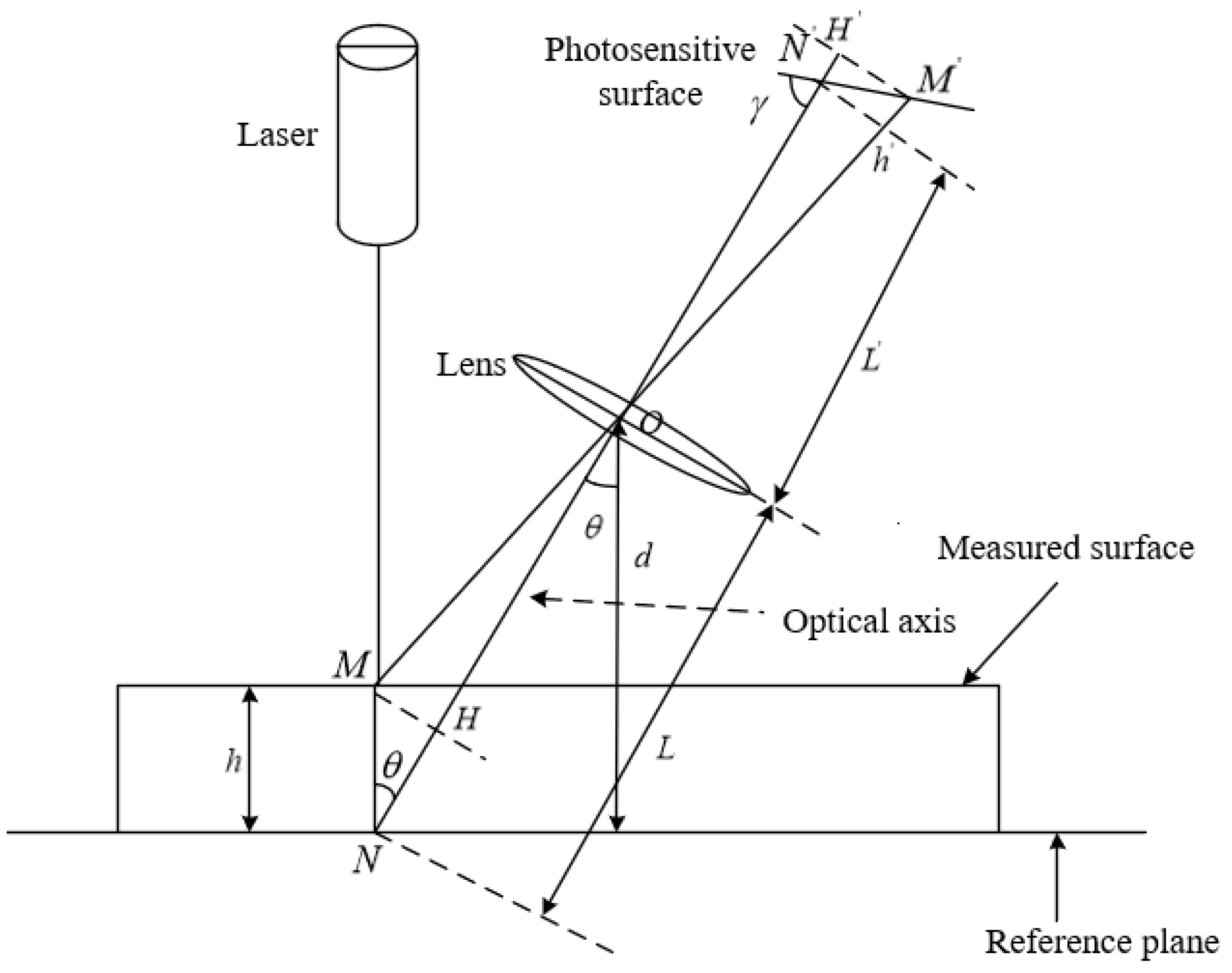
2.1. Detection Principle

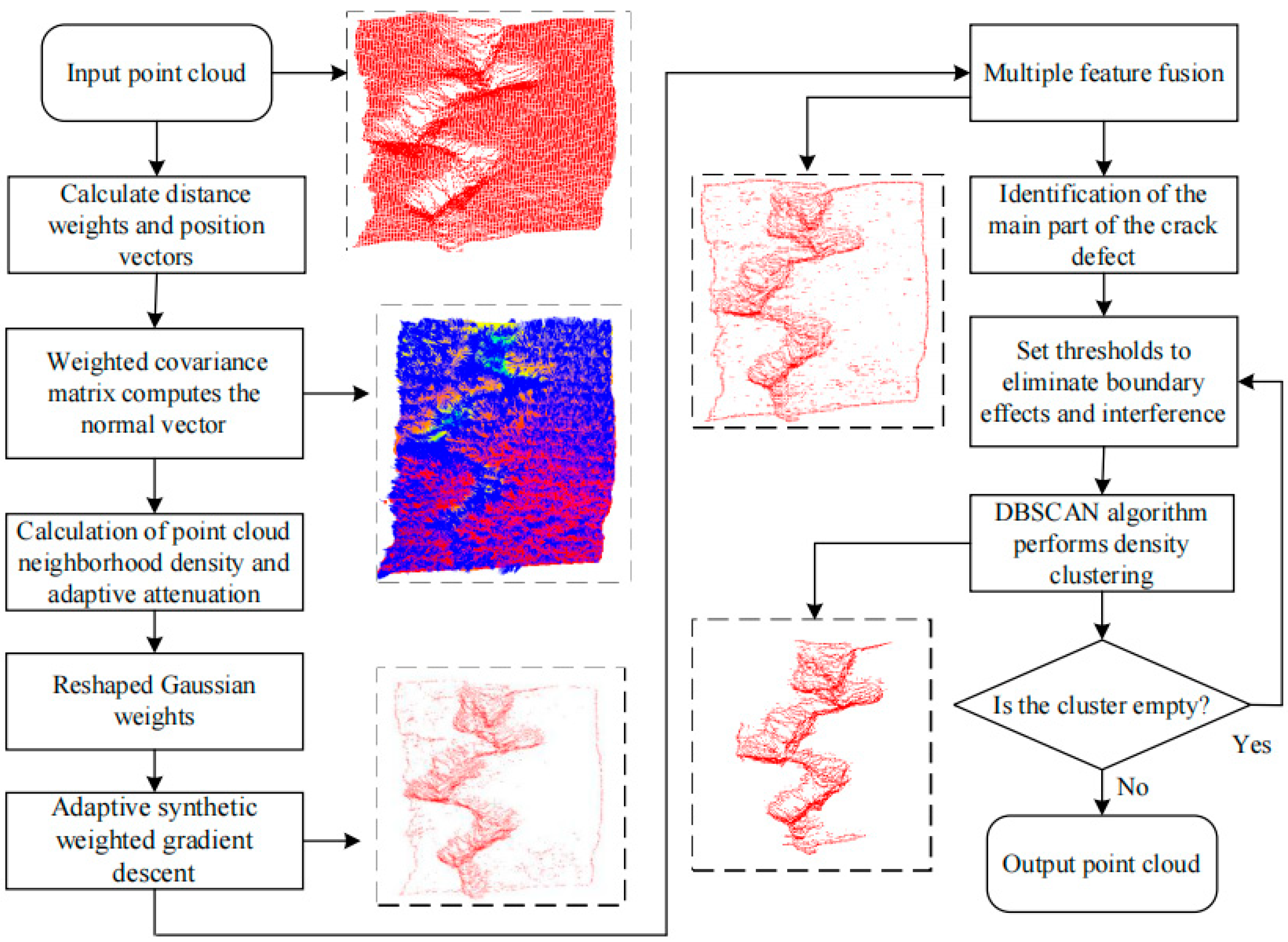
Laser triangulation is a process according to which the beam emitted by the laser passes through a lens and irradiates the object that has been placed on a moving platform. The reflected light passes through the lens again and ultimately focuses on the image sensor. Images captured by the sensor can be used to calculate the geometric features of the object’s surface. The moving platform allows the position to be adjusted of the object to be measured, which allows the accurate measurement of different areas to be achieved. The platform is illustrated in Figure 1.

The laser projects a structured line of light at an angle perpendicular to the surface of the measured object, deforming the object’s surface. The camera captures the deformed light through an imaging lens, as illustrated in Figure 2. Point $N$ represents the point where the light beam strikes the object, and point $N^{\prime }$ is the image of $N$ formed on the photosensitive surface through the imaging lens. The angle $\theta$ is the angle between $MN$ and $N{N}^{\prime }$; $\gamma$ is the angle between the extension of $N{N}^{\prime }$ and $M^{\prime }{N}^{\prime }$; $L$ is the object distance; and $L^{\prime }$ is the image distance. A perpendicular line from $M$ to the reflected light $N{N}^{\prime }$ intersects at point $H$; and a perpendicular line from $M^{\prime }$ to $N{N}^{\prime }$ intersects the extension line at point $H^{\prime }$. Moreover, $h$ is the distance between the measured surface and the reference plane and its corresponding distance on the photosensitive surface is denoted as $h^{\prime }$; $h$ represents the height of the object’s surface relative to the reference plane and plays a critical role in generating point cloud data. This allows for the precise acquisition of the object’s 3D coordinates, including height information. It is essential for analyzing the geometric characteristics of the object’s surface, such as surface roughness and flatness.

Based on the geometric principle of similarity between the triangles formed by the object and image points,$\Delta MOH\sim \Delta M^{\prime }O{H}^{\prime }$ can be established. Using the geometric relationship of similar triangles, the following equations can be derived:

$${\displaystyle \frac{MH}{M^{\prime }{H}^{\prime }}}={\displaystyle \frac{OH}{O{H}^{\prime }}}$$

(1)

$${\displaystyle \frac{hsin\theta }{h^{\prime }sin\gamma }}={\displaystyle \frac{L-hcos\theta }{L^{\prime }+h^{\prime }cos\gamma }}$$

(2)

From these, the expression for h can be obtained:

$$h={\displaystyle \frac{L{h}^{\prime }sin\gamma }{L^{\prime }sin\theta +h^{\prime }sin(\theta +\gamma )}}$$

(3)

2.2. Algorithm Flow

The surface of a casting billet has the characteristics of a rough and uneven surface. Based on the sensitivity of the gradient descent to the change in the geometric features on the surface of objects, a multi-scale adaptive gradient descent feature extraction algorithm was proposed. First, the distance weight and position vector between the points in the k-neighborhood were calculated to improve the covariance matrix. By utilizing the characteristics of the improved covariance matrix, which focuses more on local point cloud features, the normal vectors of the point clouds are calculated, and the normal variation rate between different point clouds is obtained. This normal variation rate was used to calculate the adaptive attenuation rate in the neighborhood. The point cloud k-neighborhood density weight was calculated, and the adaptive attenuation rate was fused, which can be used to reshape the Gaussian weight in the neighborhood. The improved Gaussian weight value was utilized for multi-scale feature extraction to gain the complete defect feature structure, but the acquired feature point cloud still suffered from a small amount of interference from non-crack defect point clouds. Finally, the Density-Based Spatial Clustering of Applications with Noise (DBSCAN) method was applied to eliminate boundary effects and other noise points, which can be used to extract the complete crack detail features. The algorithm flowchart is shown in Figure 3.

2.3. Normal Weighted Covariance Calculation

In regard to point cloud data, noise is a common interference, and traditional covariance matrices cannot distinguish noise from valid data. Therefore, noise can have a disproportionate effect on the calculation of the covariance matrix, which affects the accuracy of the calculation of the normal vector. The traditional PCA method may encounter the problem related to the local minimum value during eigenvalue decomposition, which leads to unstable results. This is especially the case when the covariance matrix is non-positive definite, which can result in negative eigenvalues.

To address these issues, the normal calculation method of weighted covariance was proposed. Gaussian weight assignment is carried out based on the distance of the k-neighborhood of the point cloud, which reduces the influence of noise and outliers, and enhances the robustness of normal estimation. Furthermore, the local mean is employed to capture the surface features, which can allow for more accurate capturing of local geometries than the global mean and can be used to identify detailed features. In addition, the improved method focuses on the local neighborhood of each point rather than the entire dataset, which can greatly improve the computational efficiency when processing larger-scale point cloud data. The weighted covariance matrix can also adapt to the non-uniform distribution of point cloud data, which dynamically adjusts the weights to better reflect density variations in different regions.

The nonlinear characteristics of point cloud data are mainly due to its complex and varied surface morphology and geometric structure (such as unevenness, rust, sharp edge points, cracks, etc.). The PCA method is used to calculate the normal vector of the point cloud, which assumes that the distribution of the point cloud in the local neighborhood can be approximated by a linear fitting model. However, when dealing with complex surface topography, the method cannot accurately capture local geometric information. The accuracy of normal calculations is reduced. The weighted covariance method uses Gaussian weights to dynamically assign weights based on the distance between the point and its neighboring points. The normal calculations focus more on points in the local neighborhood than on the global point cloud. The local weighted mean is applied to accurately reflect the local geometry, especially when dealing with severe crack variations. Therefore, compared to traditional methods, the weighted covariance method has a significant advantage in dealing with nonlinear features of point cloud data, which can capture local geometric information more accurately, while maintaining its robustness in regard to noise.

The traditional PCA-based covariance computation for normal calculations is as follows:

For a point set $p$ containing $k$ points, the centroid of the point set is denoted as $\overline{p}={\displaystyle \frac{1}{k}}{\displaystyle {\sum }_{i=1}^k{p}_i}$, and the covariance matrix is $C={\displaystyle \frac{1}{k}}{{\displaystyle {\sum }_{i=1}^k(p_i-\overline{p})(p_i-\overline{p})}}^T$. Here, $C$ is a 3 × 3 symmetrical positive semi-definite matrix. The eigenvalues and eigenvectors are derived from the covariance matrix, where the eigenvector corresponding to the minimum eigenvalue represents the normal direction of the point set. The improved algorithm is as follows [30,31]:

(1)

The weight and local position vector are calculated:

For each point $p_i$ in the point cloud, its k-nearest neighbor points $p_m$(where m = 1, 2,…, k) are considered, with the distance between point $p_i$ and each neighborhood point $p_m$ denoted as $d_{im}$. The weight between point $p_i$ and point $p_m$ is denoted as ${\varphi }_{im}$, and the mean ($d_{i1}$, $d_{i2}$,…, $d_{ik}$) is the average distance from $p_i$ to its k-nearest neighbors; ${\mu }_i$ is the local position vector of point $p_i$; $k$ is the number of neighborhood points.

$${\varphi }_{im}=exp(-{\displaystyle \frac{d_{im}^2}{2{(mean(d_{i1},d_{i2},\cdot \cdot \cdot ,d_{ik}))}^2}})$$

(4)

$${\mu }_i={\displaystyle \frac{{\displaystyle {\sum }_{m=1}^k{\varphi }_{im}{p}_m}}{{\displaystyle {\sum }_{m=1}^k{\varphi }_{im}}}}$$

(5)

(2)

The weighted covariance matrix is calculated:

$$co{v}_i={\displaystyle \frac{{\displaystyle {\sum }_{m=1}^k{\varphi }_{im}(p_m-{\mu }_i){(p_m-{\mu }_i)}^T}}{{\displaystyle {\sum }_{m=1}^k{\varphi }_{im}}}}$$

(6)

where $co{v}_i$ is the covariance matrix of point $p_i$.

(3)

Normal calculation and normalization:

$$norma{l}_{min}=eigen\_vecto{r}_{ij} where j=\arg \underset{j\in [1,2,3]}{min}{\lambda }_{ij}$$

(7)

$$norma{l}_i={\displaystyle \frac{norma{l}_{min}}{\left|\right|norma{l}_{min}\left|\right|}}$$

(8)

For the weighted covariance matrix $co{v}_i$ of each point $p_i$, its eigenvalues ${\lambda }_1$, ${\lambda }_2$, and ${\lambda }_3$, and corresponding eigenvectors, $eigen\_vecto{r}_{i1}$, $eigen\_vecto{r}_{i2}$, and $eigen\_vecto{r}_{i3}$, are obtained. The eigenvector corresponding to the smallest eigenvalue is taken as the normal vector of point $p_i$; where $norma{l}_i$ is the normal vector of point $p_i$. Moreover, $eigen\_vecto{r}_{min}$ is the minimum eigenvector corresponding to the minimum eigenvalue of the covariance matrix $co{v}_i$; $\left|\right|eigen\_vecto{r}_{min}\left|\right|$ is the magnitude of the eigenvector.

2.4. Adaptive Weighted Gradient Descent

2.4.1. Gradient Descent

Mathematically, the gradient of the 3D space is defined as if the function $f(x,y,z)$ has a continuous partial derivative in the space region $G$; then the gradient at the point $P(x,y,z)\in G$ in $G$ is given [32]:

$$grandf(x,y,z)=\nabla f(x,y,z)={\displaystyle \frac{\partial f}{\partial x}}\overline{i}+{\displaystyle \frac{\partial f}{\partial y}}\overline{j}+{\displaystyle \frac{\partial f}{\partial z}}\overline{k}$$

(9)

The expression for the gradient modulus length is:

$$||grandf(x,y,z)||=||\nabla f(x,y,z)||=\sqrt{{({\displaystyle \frac{\partial f}{\partial x}})}^2+{({\displaystyle \frac{\partial f}{\partial y}})}^2+{({\displaystyle \frac{\partial f}{\partial z}})}^2}$$

(10)

The gradient direction is the direction where the function $f(x,y,z)$ has the largest rate of change at the point $P(x,y,z)$, and its modulus length is the value of the maximum rate of change.

In regard to 3D point cloud processing, the point cloud exists in the form of discrete points and does not possess the characteristics of continuity. Therefore, the gradient of this point in 3D space must be calculated using estimation [33,34]. Let point $P$ be an arbitrary point in space and the set of its k-nearest neighbors in space be $Q_k=\{P_i,i\in [1,k]\}$, the simplified formula for calculating the gradient is:

$$\nabla P(x,y,z)={\displaystyle \frac{1}{k}}{\displaystyle {\sum }_{i=1}^k\frac{\overrightarrow{P{P}_i}}{{\overrightarrow{\left|\right|P{P}_i\left|\right|}}^2}}(f(P_i)-f(P))$$

(11)

where $\overrightarrow{P{P}_i}$ is the vector from point $P$ to $P_i$, and

$\overrightarrow{\left|\right|P{P}_i|{|}^2}$ is the square of the vector modulus from $P$ to $P_i$.

2.4.2. Improved Gradient Descent Method

To reduce noise interference and strengthen the local features during the gradient descent process, the Gaussian weight is introduced to adjust the influence of the neighborhood points when calculating the gradient. The Gaussian weight uses the Gaussian function to assign weights to each neighborhood point, which ensures that neighbors closer to the central point contribute more to the gradient, while distant points contribute less. This helps smooth the local features and reduce the impact of noise, effectively guiding the search direction.

To increase the applicability and robustness of feature extraction, the Gaussian weights are reconstructed using adaptive attenuation and local neighborhood density weighting of the point clouds. In regard to feature extraction and defect detection, the surface properties of different areas vary greatly. The adaptive attenuation rate can dynamically adjust the distribution of Gaussian weights based on the normal rate of change in different regions of the point cloud. In areas where the normal changes are drastically significant, i.e., areas where the surface features change significantly, the gradient calculation is more sensitive, which can better capture the features of that region.

The local density is estimated by calculating the reciprocal distance of the average of the distance from each point to its k-nearest neighbors, which can dynamically adapt to the characteristic changes in different regions in the point cloud. Especially in areas where the changes are drastic, the local density algorithm can capture these changes more sensitively, which means that it is able to better handle complex geometry in the point cloud data.

In regard to the improved algorithm, the width of the Gaussian kernel can be adjusted based on the severity of local geometric changes. In regions with drastic geometric changes, the Gaussian weights become more concentrated in regard to their neighbors, while in regions with gentle changes, the weights are more widely distributed to capture a wider range of features. The calculation process in terms of the gradient is optimized, and the accuracy and robustness of the feature extraction are improved.

The adaptive comprehensive weighted gradient descent is as follows [35,36]:

(1)

Density calculation in regard to the point cloud neighborhood:

$$densitie{s}_i={\displaystyle \frac{1}{mean(densitie{s}_i)+\epsilon }}$$

(12)

where $densitie{s}_i$ is the local density of $p_i$; $mean(densitie{s}_i)$ is the average distance from $p_i$ to its k-nearest neighbors; $\epsilon$ is a small constant that is used to prevent the denominator from being zero.

(2)

Normal change rate calculation:

$$normal\_change{s}_i=mean(||normal{s}_i-normal{s}_{i,neighbors}||)$$

(13)

Using Equations (6)–(8), the normal weighted covariance can be derived. Moreover, $normal\_change{s}_i$ is the normal change rate of $p_i$; $normal{s}_{i,neighbors}$ is the normal change rate of the k-nearest neighbors of $p_i$; $normal{s}_i$ is the normal change rate of $p_i$.

(3)

Adaptive attenuation rate calculation:

$$local\_sigm{a}_i={\displaystyle \frac{\sigma }{\sqrt{normal\_change{s}_i+\epsilon }}}$$

(14)

where $local\_sigm{a}_i$ is the adaptive attenuation rate of $p_i$; $\sigma$ is the standard deviation of the Gaussian distribution.

(4)

Comprehensive weight construction:

$$guss\_weight{s}_{ij}=exp(-{\displaystyle \frac{d_{ij}^2}{2local\_sigm{a}_i^2}})$$

(15)

$$combind\_weight{s}_{ij}=guass\_weight{s}_{ij}\cdot densitie{s}_j$$

(16)

$$normalized\_weight{s}_{ij}={\displaystyle \frac{combind\_weight{s}_{ij}}{{\displaystyle {\sum }_{j=1}^{k}combind\_weight{s}_{ij}}}}$$

(17)

where $guss\_weight{s}_{ij}$ is the difference in the Gaussian weight between $p_i$ and its nearest neighbor $p_j$-th; $combind\_weight{s}_{ij}$ is the reshaped Gaussian weight; $normalized\_weight{s}_{ij}$ is the normalized Gaussian weight; $d_{ij}$ is the distance between $p_i$ and its nearest neighbor $p_j$-th; ${\displaystyle {\sum }_{j=1}^{k}combind\_weight{s}_{ij}}$ is the sum of the combined weights of all the k − 1 nearest neighbors.

(5)

Adaptive Comprehensive Weighted Gradient Descent:

$$gradient{s}_i={\displaystyle {\sum }_{j=1}^k(\frac{exp(-\frac{d_{ij}^2}{2{\sigma }^2})\cdot densitie{s}_j}{{\displaystyle {\sum }_{m=1}^{k}exp(-\frac{d_{im}^2}{2{\sigma }^2})\cdot densitie{s}_m}})}$$

(18)

where $gradient{s}_i$ is the gradient at point $p_i$; $point{s}_i$ and $point{s}_j$ are the coordinates of point $p_i$ and its $p_j$-th nearest neighbor, respectively.

(6)

Multi-scale Feature Extraction and Detection:

$$multiscale\_gradients={\displaystyle \sum _{\sigma \in \backslash sigmas}gradients(\sigma )}$$

(19)

$$defect\_indices=\left\{i\right| \left|\right|multiscale\_gradient{s}_i\left|\right|>threshold\}$$

(20)

where $sigma$ is the array containing parameters of different scales, and $threshold$ is the gradient modulus threshold.

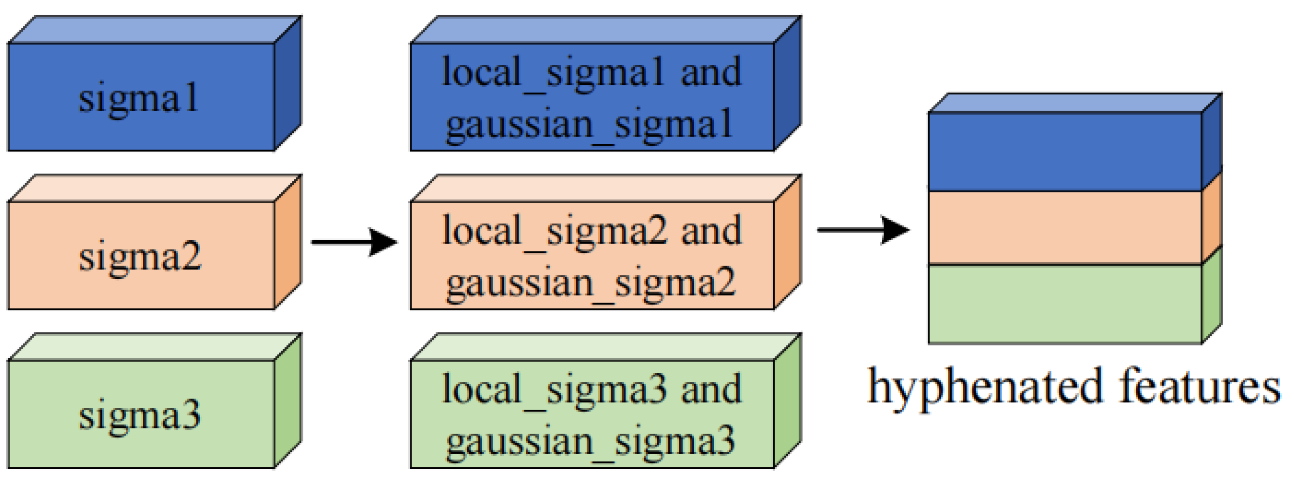
2.5. Multi-Scale Feature Fusion

To comprehensively capture the details of crack defects in point cloud data, a multi-scale feature fusion technique is introduced, as shown in Figure 4. Different sized sigma values are utilized to identify crack regions, with smaller sigma values focused on capturing local subtle features and larger sigma values focused on capturing broader global features. Gradients at different scales are cumulative, which can enable the model to gain information about both local details and global trends. Additionally, the Gaussian weight for each point is not only based on the distance, but also considers the normal variation rate of the point. The adaptive attenuation rate local_sigma was calculated, which was used to assign different weights to the features at different scales to strengthen the adaptability of the model to feature variations. The experimental results show that, as shown in

Table 1. Experimental data of the comparison at different scales.

Sigma Value	Number of Feature Points Extracted
sigma = 0.0001	27,789
sigma = 0.0002	15,087
sigma = 0.0003	10,257
sigma = 0.0004	7719

, the sigma value should be selected within the range of 0.0001 to 0.0004. The weighted gradient is calculated by combining the density of the point cloud and the normal rate of change. Therefore, the model can assign weights to features at different scales to effectively capture the local and global features, thereby improving the accuracy and robustness of defect detection.

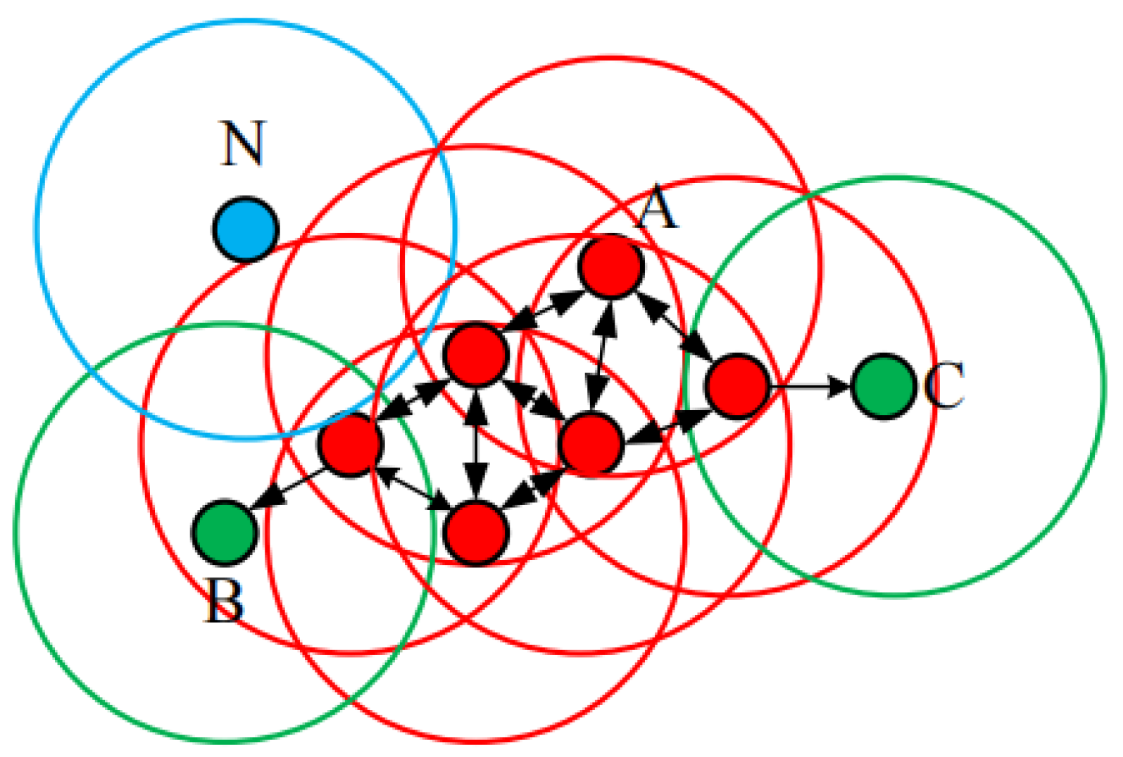
2.6. DBSCAN Clustering

Density-Based Spatial Clustering of Applications with Noise (DBSCAN) is a density-based clustering algorithm that can identify arbitrarily shaped clusters and identify noise points. Clusters are made up of density-connected points. Points within the same cluster are sufficiently close to each other, while clusters are separated by low-density regions [37,38].

DBSCAN performs clustering by setting two main parameters: ε (neighborhood size) and MinPts (the minimum number of points required to form a cluster). The algorithm first randomly selects a point and then finds the neighboring points of the point within the ε distance. If the number of points in the neighborhood is greater than or equal to MinPts, the point becomes a core point and begins to form clusters. The core point and all the points in its neighborhood are added to the new cluster, and the cluster is expanded until all the points are accessed. Points not included in any cluster are considered noise points. The clustering process is illustrated in Figure 5, where A is the core point, B and C are border points, and N is an outlier [39].

3. Analysis and Discussion

3.1. Experimental Platform

To validate the extraction effect of the proposed algorithm on the surface cracks of the casting billet, a 3D measurement system (Figure 6a) was built. The measurement system is composed of a 3D laser displacement sensor and a mobile platform, as shown in Figure 6a. The 7060D 3D laser displacement sensor, from SinceVision company (Shenzhen, China), was used for the detection experiment. This sensor consists of a linear structured light and a binocular camera.

The wavelength of the light source is 405 nm. The binocular camera has a repeatability of 2.5 $\mathsf{\mu }\mathrm{m}$ in regard to the X axis and 0.2 $\mathsf{\mu }\mathrm{m}$ in regard to the Z axis. The point cloud dataset is collected according to the laser triangle reflection principle, as shown in Figure 6c. The tested sample is a continuous cast steel block with cracks on the surface, as shown in Figure 6b.

3.2. Evaluation Indicators

Precision (P), recall (R), F-measure (F), Mean Squared Error (MSE), and Mean Absolute Error (MAE) were applied as evaluation indicators to comprehensively measure the performance of the improved normal calculation and crack extraction method [40,41].

$$P={\displaystyle \frac{TP}{TP+FP}}\times 100\%$$

(21)

$$R={\displaystyle \frac{TP}{TP+FN}}\times 100\%$$

(22)

$$F=2\times ({\displaystyle \frac{P\times R}{P+R}})$$

(23)

$$MSE={\displaystyle \frac{1}{n}}{\displaystyle {\sum }_{i=1}^n{(y_i-{\widehat{y}}_i)}^2}$$

(24)

$$MAE={\displaystyle \frac{1}{n}}{\displaystyle {\sum }_{i=1}^n|y_i-{\widehat{y}}_i|}$$

(25)

The True Positive (TP) is the number of defect-related point clouds that are correctly identified by the algorithm, i.e., the overlap between the defect-related point clouds detected by the algorithm and the actual defect-related point clouds. The False Positive (FP) is the number of non-defect-related point clouds that are incorrectly identified as defects by the algorithm, i.e., the portion of defect-related point clouds detected by the algorithm that are not actual defect-related point clouds. The False Negative (FN) is the number of actual defect-related point clouds that are not identified by the algorithm, i.e., the portion of actual defect-related point clouds that were not detected by the algorithm. Moreover, $n$ is the number of sample point clouds. In addition, $y_i$ is the original normal point cloud without the introduction of noise, and ${\widehat{y}}_i$ is the normal point cloud generated after introducing noise. The number of point clouds at the defect calibration site is 11,401.

3.3. Normal Calculation Comparison Experiment

To verify the accuracy and robustness of the improved weighted covariance method for calculating normal vectors, as well as the generalization of the algorithm’s application scenarios, under the same experimental conditions, different proportions (15–30%) of salt-and-pepper noise were introduced into the same dataset. The resulting normal vector calculation outcomes were compared to the traditional original normal vector calculation results through the use of error analysis [42,43,44]. The experimental results are shown in

Table 2. Experimental data for normal calculation comparison.

Algorithm	Noise Ratio/%	MSE/%	MAE/%
①	15	51.69	39.50
②		51.37	38.57
①	20	52.53	41.41
②		52.22	40.37
①	25	54.13	43.71
②		53.01	41.93
①	30	55.05	45.47
②		54.07	43.85

. The symbol ① represents the traditional PCA algorithm, while ② represents an improved algorithm for calculating the normal vector using weighted covariance.

As can be seen in Table 2, the error of the algorithm increases with the increase in the proportion of interference noise introduced. However, the MSE value and MAE value of the improved algorithm are smaller than those of the traditional algorithm.

With the rise in the proportion of introduced noise, the advantages of the improved algorithm become more and more prominent. It is verified that the improved algorithm can reduce the influence of noise and improve the stability and accuracy of the outcomes.

3.4. Multi-Scale Comparative Experiment

Under the same experimental conditions, the sigma value of the key parameter was changed to assess the influence of different scale parameters on the feature extraction of crack defects on the surface of the casting billet. In regard to the experiment, each sigma value corresponds to a specific scale level, and the Gaussian weight and adaptive attenuation rate (local_sigma) were calculated independently. As the core parameter in the Gaussian weight calculation, the sigma value significantly affects the algorithm’s ability to capture feature information. It determines the sensitivity of the algorithm to local details and global trends during the feature extraction process.

As shown in Table 1 and Figure 7, a smaller sigma value (0.0001) makes the gradient descent more sensitive to changes in the geometric features of the object’s surface, which can be used to clearly identify details, such as rust and minor scratches (Figure 7a). However, this high sensitivity also leads to excessive retention of feature details in the point cloud, which could cause an excessive number of points and over-recognition. A larger sigma value (0.0004) can capture low-frequency trends, such as the overall shape shown in Figure 7d, which could lead to fewer feature points in the crack point cloud and under-identification. To fully capture the multi-scale features of cracks, sigma1 = 0.00025, sigma2 = 0.0003, and sigma3 = 0.00035 in the sigma array in Equation (19) are set, and the feature extraction is shown in Figure 8d.

3.5. Gradient Descent Comparison Experiment

To compare the effects of different gradient descent calculation methods on the extraction of crack defects, our method was compared to the finite difference method [45], nearest neighbor method [46], and Gaussian weight method [47].

From

Table 3. A comparison of the experimental data for different gradient algorithms.

Algorithm	Number of Feature Points Extracted
Finite Difference Method	7889
Nearest Neighbor Method	12,365
Gaussian Weight Method	8756
Improved Method	11,927

and Figure 8, after processing the point cloud data using the finite difference method, the number of feature clouds is 7889. Errors are generated due to the discretization of point cloud data, which triggers inaccurate feature extraction. This is the case especially when the point cloud density is uneven, which brings about the severe loss of feature extraction details. The nearest neighbor method can maintain the local features well when processing the point cloud data, and the number of feature point clouds obtained is 12,365. However, this method is susceptible to noise and outlier interference during the process of processing the point clouds, which affects the accuracy of the feature extraction. The Gaussian weight method can effectively smooth the point cloud data and reduce the influence of noise by assigning weights to the point cloud data through the use of the Gaussian function, and the number of feature point clouds obtained is 8756. However, the selection of Gaussian weights has a great impact on the performance of the algorithm, and improper weight selection may lead to feature extraction bias.

Compared to the above methods, the improved method has excellent performance in terms of the accuracy and robustness of the feature extraction, with 11,927 feature point clouds extracted. It can more clearly extract the main features of the point cloud, while also demonstrating good performance in handling noise and outliers. This indicates that the proposed method has higher efficiency and accuracy in regard to point cloud feature extraction.

3.6. Algorithm Comparison Experiment

To validate the superiority of the improved algorithm, comparative experiments were conducted on sample 1 (Figure 9), under the same experimental conditions. The experimental data are displayed in Figure 10 and Figure 11,

Table 4. Comparison of experimental data for the different algorithms.

Algorithm	Number of Feature Points	Number of Overlapping Point Clouds (TP)	Number of False Negative Point Clouds (FN)	Number of False Positive Point Clouds (FP)
Curvature Algorithm	8254	5728	5673	2526
RANSAC Algorithm	8784	8337	3064	447
Region-Growing Algorithm	7923	7603	3798	320
Improved Algorithm	10,767	10,410	991	357

and

Table 5. Comparison of feature extraction performance of the different algorithms.

Algorithm	Precision/%	Recall/%	F/%
Curvature Algorithm	69.39	50.24	58.47
RANSAC Algorithm	94.90	73.13	82.76
Region-Growing Algorithm	95.96	66.69	79.57
Improved Algorithm	96.68	91.31	93.92

, and the red box line is the difference in terms of the comparison area.

As shown in Figure 10 and Figure 11, the RANSAC algorithm is prone to misjudge the non-crack region as a defect during the extraction of crack defects in complex planes. The curvature method is easily influenced by uneven and rusty surfaces, which causes changes in curvature and normal vectors, resulting in recognition interference. The region-growing algorithm for defect identification effectively addresses the issue of abrupt normal vector changes due to steep object boundaries, as well as the point cloud misidentification problem caused by the sensitivity of the curvature to surface variations. However, this method may cause under-recognition of the main crack features. Through the extraction of multi-scale features, our algorithm acquires all of the crack features, and applies DBSCAN density clustering to eliminate boundary effects and other noises. The crack extraction effect is significantly improved compared to the other algorithms.

Table 4 reveals that the point cloud data gained by the curvature algorithm could cause a large number of incorrectly detected point clouds, due to the uneven surface of the measured object. The extraction effect of the RANSAC algorithm and region-growing algorithm is better. However, large numbers of crack defect features are still under-recognized. The improved algorithm has the largest number of detected feature point clouds, and the least number of error point clouds, which means that it achieves the best level of extraction.

As can be seen in Table 5, the precision and recall of the improved algorithm are 96.68% and 91.31%, respectively, which are the highest values among the algorithms. Compared to the other algorithms, the precision of the improved algorithm is 0.72% higher than the region-growing algorithm, which has the highest precision among the other algorithms. This finding validates that it has an excellent level of accuracy in terms of crack area identification. The recall of the improved algorithm is 18.18% higher than the RANSAC algorithm. The large improvement in the recall rate proves that the improved algorithm can identify most of the crack areas. The F-value of the improved algorithm is 93.92%, which is 11.16% higher than that of the RANSAC algorithm. The comprehensive performance of the improved algorithm is much better than that of the other algorithms. The improved algorithm has excellent crack feature extraction performance.

4. Conclusions

To improve the detection efficiency in terms of corner cracks in casting billets and enhance the feature extraction of fine cracks on rough surfaces, a multi-scale adaptive gradient descent crack feature extraction algorithm was proposed. The following conclusions can be drawn:

(1)

The covariance matrix is optimized to increase the accuracy and stability of the normal calculation. The traditional PCA covariance matrix has limitations when dealing with the uneven distribution of point clouds. The improved algorithm optimizes the covariance matrix by calculating the position distance weight and position vector. It can better adapt to the non-uniformity of point cloud data, which significantly increases the accuracy and stability of the normal calculation. In the case of complex surfaces and noise interference, this optimization ensures the robustness of the normal calculation and provides a more reliable basis for subsequent crack detection;

(2)

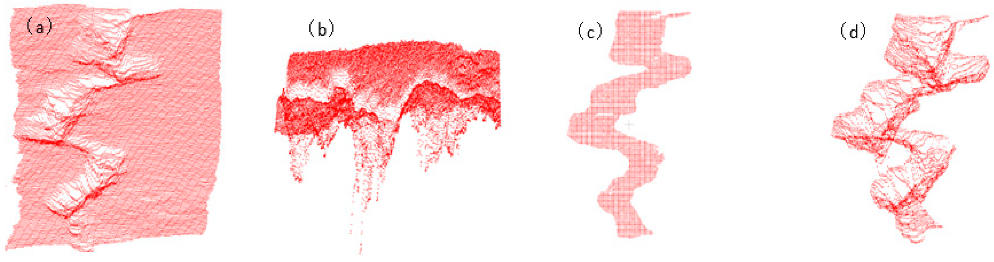
Multi-scale feature extraction is used to enhance the accuracy of crack point cloud feature extraction. By changing the sigma values, the features are obtained at different scales, and the detailed features are fused. The method can capture the subtle changes in cracks at different scales and avoid the limitations of the single-scale method. Rough surfaces and cracks exhibit different characteristics at different scales. By integrating the characteristics of different scales, the algorithm can describe the geometric characteristics of cracks more comprehensively, thereby significantly increasing the accuracy of feature extraction of crack point clouds;

(3)

The adaptive comprehensive weighted gradient descent method is utilized to dynamically adjust the gradient descent of point clouds in different neighborhoods, while smoothing noise and strengthening local features. It not only boosts the accuracy of feature extraction, but also enhances the robustness of the algorithm as well. Through adaptive gradient descent, the algorithm can better handle noise and complex surfaces. It has a stable crack detection capability, which can effectively reduce false detections and missed detections;

(4)

The experimental results indicate that the precision of the improved algorithm is 0.72% higher than that of the region-growing algorithm. Compared to the RANSAC algorithm, the improved algorithm has an enhancement of 18.18% in regard to the recall rate and 11.16% in regard to the F-value, which has great crack feature extraction performance in order to extract fine cracks with rough surfaces.

In regard to practical applications, the multi-scale feature extraction process needs to be calculated multiple times at different scales, which could lead to a significant increase in computational complexity. In the future, a distributed computing framework could be applied to optimize the feature fusion strategy and reduce redundant computing.

References

1. Kumar, S.; Rai, R.K. Minimization of cracks on the narrow face of cast slab for HCMA grade steel. Trans. Indian Inst. Met. 2024, 77, 4033–4039. [Google Scholar] [CrossRef]
2. Wang, M.; Zhang, H.; Liu, H.; Xu, L. Effect of temperature and solidification structure evolution of S355 slabs with different corner shapes on transverse corner cracks. Metals 2022, 12, 1383. [Google Scholar] [CrossRef]
3. Liu, G.; Liu, Q.; Ji, C.; Chen, B.; Li, H.; Liu, K. Application of a novel chamfered mold to suppress corner transverse cracking of micro-alloyed steel slabs. Metals 2020, 10, 1289. [Google Scholar] [CrossRef]
4. Tripathi, P.K.; Kumar, D.S.; Rajendra, T.; Vishwanath, S.C. Mitigation of corner cracking in continuously cast steel slabs through strain induced crack opening test. J. Fail. Anal. Preven 2023, 23, 1918–1931. [Google Scholar] [CrossRef]
5. Zhang, F.; Yang, S.; Li, J.; Liu, W.; Wang, T.; Yang, J. Formation mechanism and control of transverse corner cracks in fine blanking steel. J. Mater. Res. Technol. 2022, 18, 1137–1146. [Google Scholar] [CrossRef]
6. Du, C.; Wang, C.; Li, B.; Ma, B.; Zhang, J. Effect of the temperature field and cooling rate along casting direction surface transverse crack of microalloyed steel. J. Iron Steel Res. 2018, 30, 523–528. [Google Scholar]
7. Gontijo, M.; Hoflehner, C.; Ilie, S.; Six, J.; Sommitsch, C. Analysis of transverse corner cracks from continuous casting process and comparison to laboratory experiments. Eur. J. Mater. 2022, 2, 222–233. [Google Scholar] [CrossRef]
8. Deng, L.; Sun, T.; Yang, L.; Cao, R. Binocular video-based 3D reconstruction and length quantification of cracks in concrete structures. Autom. Constr. 2023, 148, 104743. [Google Scholar] [CrossRef]
9. Hu, K.; Chen, Z.; Kang, H.; Tang, Y. 3D vision technologies for a self-developed structural external crack damage recognition robot. Autom. Constr. 2024, 159, 105262. [Google Scholar] [CrossRef]
10. Qi, C.R.; Su, H.; Mo, K.; Guibas, L.J. Pointnet: Deep learning on point sets for 3d classification and segmentation. In Proceedings of the 2017 IEEE Conference on Computer Vision and Pattern Recognition (CVPR), Honolulu, HI, USA, 21–26 July 2017. [Google Scholar] [CrossRef]
11. Qi, C.R.; Yi, L.; Su, H.; Guibas, L.J. Pointnet++: Deep hierarchical feature learning on point sets in a metric space. Adv. Neural Inf. Process. Syst. 2017, 30, 5105–5114. [Google Scholar] [CrossRef]
12. Xu, M.; Zhang, J.; Zhou, Z.; Xu, M.; Qi, X.; Qiao, Y. Learning geometry-disentangled representation for complementary understanding of 3d object point cloud. Proc. AAAI Conf. Artif. Intell. 2021, 35, 3056. [Google Scholar] [CrossRef]
13. Ma, X.; Qin, C.; You, H.; Ran, H.; Fu, Y. Rethinking network design and local geometry in point cloud: A Simple Residual MLP Framework. arXiv 2022, arXiv:2202.07123. [Google Scholar]
14. Zhou, Y.; Ji, A.; Zhang, L. Sewer defect detection from 3D point clouds using a transformer-based deep learning model. Autom. Constr. 2022, 136, 104163. [Google Scholar] [CrossRef]
15. Hu, Q.; Hao, K.; Wei, B.; Li, H. An efficient solder joint defects method for 3D point clouds with double-flow region attention network. Adv. Eng. Inform. 2022, 52, 101608. [Google Scholar] [CrossRef]
16. Zeng, S.; Wang, W.; Yin, T.; Peng, J.; Liu, Y.; Zhang, J. A measurement method for rail wear based on point cloud registration and nearest neighbor search. J. Yanshan Univ. 2025, 49, 55–65. Available online: https://kns.cnki.net/kcms2/article/abstract?v=HUa8WMVVXl036yC2aoLA72tBDUrrVAJdOIXMP4UeQ1skGzUR1NvumyJnDNf6tcRfCAXuMrgpQY8jKCq2_msp8tnIYFXkabVfe36zFvuqhsf-QPeO-zIjWGIFCNRMdtYf0jC3v4IUmLIr1w2o5GPLbguojl002PBz0yA8oxPVMZ0hToRWbonP-tVLnFynyfzv&uniplatform=NZKPT&language=CHS (accessed on 14 March 2025).
17. Cai, S.; Hao, F.; Shi, T. Partition based on features of neighborhood point and the corresponding cloud registration of aero-engine damaged blade point. J. Beijing Univ. Aeronaut. Astronaut. 2024. [Google Scholar] [CrossRef]
18. Yang, J.; Zhang, J.; Song, T.; Ding, H. A point cloud registration algorithm considering multi-allowance constraints for robotic milling of complex parts. Robot. Comput.-Integr. Manuf. 2025, 92, 102885. [Google Scholar] [CrossRef]
19. Wu, Q.; Hu, Z.; Qin, X.; Huang, B.; Dong, K.; Shi, A. Surface defects 3D localization for fluorescent magnetic particle inspection via regional reconstruction and partial-in-complete point clouds registration. Expert Syst. Appl. 2024, 238, 122225. [Google Scholar] [CrossRef]
20. Zhang, T.; Xia, R.; Zhao, J.; Fu, S.; Xu, Z. Weld surface quality inspection based on structured light. Modul. Mach. Tool Autom. Manuf. Tech. 2022, 1, 81–84. [Google Scholar] [CrossRef]
21. Yang, L.; Liu, Y.; Peng, J.; Liang, Z. A novel system for off-line 3D seam extraction and path planning based on point cloud segmentation for arc welding robot. Robot. Comput.-Integr. Manuf. 2020, 64, 101929. [Google Scholar] [CrossRef]
22. Ma, W.; Wang, J.; Zhang, J.; Ma, Y.; Zhang, Z. Feature extraction from point cloud based on improved normal vector. Sci. Surv. Mapp. 2021, 46, 84–90+146. [Google Scholar] [CrossRef]
23. Wu, Y.; Ma, H.; Guo, J.; Ye, H.; Yang, X.; Yao, Q. Method for extracting point clouds of inspection pits based on normal vector region clustering segmentation. Yangtze River 2023, 54, 113–118. [Google Scholar] [CrossRef]
24. Yu, M.; Cui, X.; Wu, L.; Wu, S. 3D recognition algorithm based on curvature point pair features. Laser Optoelectron. Prog. 2023, 60, 222–229. [Google Scholar] [CrossRef]
25. Luo, Q.; Zhang, C.; Luo, J. Indoor 3D point cloud plane segmentation based on boundary feature constraints. Laser J. 2024, 45, 106–112. [Google Scholar] [CrossRef]
26. Li, Z.; Wang, T.; Hu, K.; Li, X.; Wang, X. Lidar object real-time detection method under complex environment. Laser J. 2018, 39, 41–46. [Google Scholar] [CrossRef]
27. Deng, B.; Wang, Z.; Jin, Y.; Chen, Y.; Wu, Q.; Li, H. Feature extraction method of laser scanning point cloud based on morphological gradient. Laser Optoelectron. Prog. 2018, 55, 239–245. [Google Scholar] [CrossRef]
28. Chen, H.; Ding, Q.; Pan, L. Edge optimized extraction from the organized point-cloud data base on gradient clustering. Chin. J. Instrum. 2022, 43, 165–174. [Google Scholar] [CrossRef]
29. Zhang, B.; Cai, L.; Wang, X.; Wu, J. Automatic extraction algorithm of step lines from point cloud in open-pit mine based on gradient of scalar field. Bull. Surv. Mapp. 2023, 7, 63–68. [Google Scholar] [CrossRef]
30. Huang, Z.; He, H.; Zhang, X. Linear feature extraction of LiDAR point cloud based on PCA. Bull. Surv. Mapp. 2024, 2, 146–150. [Google Scholar] [CrossRef]
31. Peng, K.; Tan, J.; Zhang, G. A Method of Curve Reconstruction Based on Point Cloud Clustering and PCA. Symmetry 2022, 14, 726. [Google Scholar] [CrossRef]
32. Marghani, K.; Dlay, S.S.; Sharif, B.S.; Sims, A.J. Automated morphological analysis approach for classifying colorectal microscopic images. Proc. SPIE-Int. Soc. Opt. Eng. 2003, 52, 240–249. [Google Scholar] [CrossRef]
33. Lu, J.; Qian, J.; Han, W. Discrete gradient method in solid mechanics. Int. J. Numer. Methods Eng. 2008, 74, 619–641. [Google Scholar] [CrossRef]
34. Qian, J.; Lu, J. A stabilized formulation for discrete gradient method. Int. J. Numer. Methods Biomed. Eng. 2011, 27, 860–873. [Google Scholar] [CrossRef]
35. Zhu, D.; Wang, D.; Chen, Y.; Xu, Z.; He, B. Research on Three-Dimensional Reconstruction of Ribs Based on Point Cloud Adaptive Smoothing Denoising. Sensors 2024, 24, 4076. [Google Scholar] [CrossRef]
36. Cabo, C.; Ordóñez, C.; Sáchez-Lasheras, F.; Roca-Pardiñas, J.; de Cos-Juez, J. Multiscale Supervised Classification of Point Clouds with Urban and Forest Applications. Sensors 2019, 19, 4523. [Google Scholar] [CrossRef]
37. Zhou, N.; Jiang, P.; Jiang, S.; Shu, L.; Ni, X.; Zhong, L. An Identification and Localization Method for 3D Workpiece Welds Based on the DBSCAN Point Cloud Clustering Algorithm. J. Manuf. Mater. Process 2024, 8, 287. [Google Scholar] [CrossRef]
38. Xu, X.; Zhang, R.; Gao, C.; Chen, Z. Centerline Extraction Method of Structured Light Stripe Based on GWGCGM and DBSCAN. Appl. Laser. 2024, 44, 164–171. [Google Scholar] [CrossRef]
39. Ester, M.; Hans-Peter, K.; Jorg, S.; Xu, X. A Density-Based Algorithm for Discovering Clusters in Large Spatial Databases with Noise; AAAI Press: Washington, DC, USA, 1996; pp. 226–231. [Google Scholar]
40. Flach, P.A.; Meelis, K. Precision-recall-gain curves: PR analysis done right. Adv. Neural Inf. Process. Syst. 2015, 28, 838–846. [Google Scholar]
41. Fouhey, D.F.; Gupta, A.; Hebert, M. Data-Driven 3D Primitives for Single Image Understanding. In Proceedings of the 2013 IEEE International Conference on Computer Vision, Sydney, Australia, 1–8 December 2013; pp. 3392–3399. [Google Scholar] [CrossRef]
42. Wang, W.; Lu, X.; Shao, D.; Liu, X.; Dazeley, R.; Robles-Kelly, A.; Pan, W. Weighted point cloud normal estimation. In Proceedings of the 2023 IEEE International Conference on Multimedia and Expo (ICME), Brisbane, Australia, 10–14 July 2023; pp. 2015–2020. [Google Scholar] [CrossRef]
43. Zhou, L.; Sun, G.; Li, Y.; Li, W.; Su, Z. Point cloud denoising review: From classical to deep learning-based approaches. Graph. Models 2022, 121, 101140. [Google Scholar] [CrossRef]
44. Li, Q.; Feng, H.; Shi, K.; Gao, Y.; Fang, Y.; Liu, Y.; Han, Z. Learning signed hyper surfaces for oriented point cloud normal estimation. IEEE Trans. Pattern Anal. Mach. Intell. 2024, 46, 9957–9974. [Google Scholar] [CrossRef]
45. Pan, X.; Ling, T.; Zhang, L.; Lou, Y. Forward simulation and waveform feature analysis of cracks in lining structures. J. Transp. Sci. Eng. 2024, 41, 1605–1609. [Google Scholar]
46. Zhou, Y.; Du, J.; Tao, Y. Method for precipitation forecast based on improved k-nearest neighbor algorithm. Comput. Eng. Des. 2020, 41, 1605–1609. [Google Scholar] [CrossRef]
47. Zhang, J.; Quan, T. A local Gaussian distribution model for image registration. Chin. J. Eng. Math. 2024, 41, 421–431. [Google Scholar] [CrossRef]
Figure 1. Laser measurement system schematic diagram.
Metals 15 00324 g001
Figure 2. Diagram of direct laser triangulation principle.
Metals 15 00324 g002
Figure 3. Algorithm flowchart.
Metals 15 00324 g003
Figure 4. Multi-scale feature fusion.
Metals 15 00324 g004
Figure 5. The clustering process of DBSCAN.
Metals 15 00324 g005
Figure 6. Experimental equipment: (a) measurement platform; (b) steel block sample; (c) 3D point cloud of the steel block.
Metals 15 00324 g006
Figure 7. Comparison of detection effects at different scales: (a) sigma = 0.0001; (b) sigma = 0.0002; (c) sigma = 0.0003; (d) sigma = 0.0004.
Metals 15 00324 g007
Figure 8. Comparison of different gradient descent algorithms: (a) finite difference method; (b) nearest neighbor method; (c) Gaussian weight method; (d) improved method.
Metals 15 00324 g008
Figure 9. Experimental dataset: (a) top view of the dataset; (b) side view of the dataset; (c) top view of the defect-marked area; (d) front view of the defect-marked area.
Metals 15 00324 g009
Figure 10. Comparison of the detection results from the top view: (a) curvature algorithm; (b) RANSAC algorithm; (c) region-growing algorithm; (d) improved algorithm.
Metals 15 00324 g010
Figure 11. The 3D detection effect: (a) curvature algorithm; (b) RANSAC algorithm; (c) region-growing algorithm; (d) improved algorithm.
Metals 15 00324 g011