Abstract
Determining the stress–strain curve and other plastic properties using instrumented indentation techniques has long been a topic of active study. The potential to use small, geometrically simple specimens and to characterize a component under service without the need to remove material for specimen preparation makes this methodology highly attractive to many industries. In this study, a data-driven approach that leverages machine learning and finite element analysis was used to construct a model called ‘Brilearn’ that predicts the stress–plastic strain curve of metallic materials. The framework consists of a novel model for predicting the hardening curve, the classical Tabor model for predicting the yield stress for materials with yield stress lower than 100 MPa, and an XGBoost model for predicting the yield stress for metals with yield stress higher than 100 MPa. The model was validated against experimental data on Al1100, Al6061-T6, Al7075-T6, and brass and copper alloys, features error predictions of 8.4 ± 8.5% for the yield stress and 3.2 ± 4% for a complete curve ranging from to . The model is especially suited for the determination of the stress–plastic strain curves for components in service since only two simple indentation tests are required.
1. Introduction
Mechanical testing techniques have been integral to the characterization of metallic materials, providing essential insights into their mechanical properties and behavior under load. Among these techniques, instrumented indentation has emerged as a tool for assessing strength in a relatively simple and straightforward manner. Originating from the seminal work of Johann A. Brinell, the Brinell hardness test laid the groundwork for subsequent advancements in indentation testing methodologies [1].
The Brinell indentation test is a method used to measure the hardness of a material. A hard sphere, usually made of tungsten carbide, is pressed against the surface of the material with a predetermined load for a specified amount of time. The diameter of the resulting indentation left on the material’s surface is measured optically and is used to calculate the Brinell hardness number using the following formula:
where P is the applied force, D is the indenter diameter, and d is the indentation trace diameter.
For an adequate Brinell test, the material surface must be flat, bulky, and free from contaminants. A suitable testing machine capable of applying and releasing the specified load accurately and normal to the specimen surface, along with a calibrated microscope, is also required [2].
Instrumented indentation techniques (IIT) can be divided into two main categories: the indentation scale, which goes through nano-indentation, micro-indentation, and macro-indentation, and whether the loading procedure is continuous or discrete, where the former is more common in nano-indentation, and the latter, in macro-indentation.
The field of macro-indentation, and especially the Brinell hardness method, has evolved throughout the 20th century by both developing empirical and theoretical frameworks for hardness testing [3,4,5] and the advent of modern instrumentation capable of precise force and trace measurements.
Simultaneously, Nanoindentation has garnered widespread attention for its ability to probe material properties at the nanoscale, offering insights into phenomena such as phase transformations, strain rate effects, and size-dependent mechanical behavior [6,7]. Nanoindentation has been found to be particularly advantageous for characterizing thin films where traditional mechanical testing methods are inadequate. Recent studies have continued to demonstrate the effectiveness of classical [8,9,10] and machine learning-aided [11,12,13] nanoindentation in extracting elastic-plastic and tribological properties. Although nano-indentation techniques bear a resemblance to the instrumentation techniques and mechanical behavior inverse extraction methods, their great effectiveness in characterizing localized behavior may be disadvantageous when one wishes to determine the effective bulk mechanical response. This is due to material heterogeneities such as grain boundaries of surface roughness. For determining bulk material response, for larger specimens, macro-indentation may be preferable.
When dealing with the mechanical characterization of metals, one sought-after ability is to measure the stress–strain curve and other plastic properties using instrumented indentation techniques due to the ability to use small, geometrically simple specimens and to characterize a component under service without the need to remove material for specimen preparation [14]. However, the complex nature of the stress and strain fields developed during an indentation test makes this matter a nontrivial one. Nevertheless, over the last two decades, research has been conducted in this regard, and several models for predicting plastic behavior from instrumented indentation techniques have been developed. These models can be divided into the following categories:
- Finite element-based inverse modeling of an IIT [15,16,17,18]. This approach consists of guessing an initial plastic material model and hardening curve and iteratively adjusting the model’s constant until the computed force-displacement curve converges to the experimental one.
- Coupled FE-Bayesian framework approach [19].
- Deep learning approach [14,20,21,22,23,24]. This approach consists of generating data of the stress–strain curve and its equivalent IIT force–displacement curve using finite element modeling of instrumented indentation tests and using this data to train a neural network architecture to predict stress–strain curve for a given force-displacement curve and possibly other parameters. The main differences between the various publications that implement this approach stem from the material model and its constant range used in the data generation procedure, the neural network architecture implemented, and the validation procedure.
These approaches have overall shown good performance in predicting the plastic behavior of materials. However, all these models require a continuous measurement of the force-displacement curve of an indenter to predict the plastic behavior. Continuous measurement generally requires specialized and expensive equipment and specialized specimen preparation and must be conducted in a laboratory setting. In many cases, especially for in-service structures or devices, only simplified discrete indentation measurements are possible. When it comes to stress–strain curve prediction, two main options are available. The first is the Tabor model, which is an empirical model that utilizes the following relations between a force–trace diameter pair and its corresponding stress–strain pair [25]:
In (2), are the stress and plastic strain while, P is the force, d the trace and D the indenter diameter. The second option is using inverse FE modeling of an indentation experiment to iteratively find the flow stress that produces a trace diameter equal to the experimental trace diameter for every indentation experiment. Although this approach has been proven successful [26,27], it requires both time and expertise. In addition, to the authors’ best knowledge, no other method exists for predicting the stress–strain curve of a material using several discrete indentation tests.
One way of addressing this prediction problem is by using data-driven and machine-learning tools. Machine learning refers to traditional techniques and algorithms used to enable computers to learn from data and make predictions or decisions without being explicitly programmed. These powerful tools have been utilized in the scientific community in order to innovatively identify mechanical parameters [20,23,28,29], mechanical strength [30,31], physical properties [32], and accelerated materials discovery [33,34].
These algorithms necessitate quality data, which is divided into the following groups:
- A train group, with which the model ‘learns’ how to make predictions.
- A validation group, utilized to fine-tune a model’s hyperparameters (i.e., parameters that control the learning process and affect how the algorithm operates).
- A test group is used to evaluate the model’s prediction capabilities using evaluation metrics (such as mean squared error) and thus see how well it generalizes to unseen data.
In this study, we present a novel data-driven approach that leverages machine learning based on finite element analysis data to predict the stress–strain curve of metallic materials from several Brinell hardness tests. By comparison to experimental data, it is demonstrated that the proposed methodology can be used to determine the stress–strain response of a wide range of metallic materials with good accuracy.
The manuscript is structured as follows: Following this introduction, in Section 2, the methodology used in this study is presented. Section 3 outlines the numerical framework for generating the indentation data required for subsequent modeling. In Section 4, the two core machine learning models used in this work are introduced. Section 5 features a performance analysis and a comparative discussion of the aforementioned models. Summary and conclusions are given in Section 6.
2. Methodology
The methodology for the construction of a model capable of predicting the stress–strain curve of metallic materials from several Brinell hardness tests is as follows:
- A database of Brinell indentation force–diameter trace pairs was created. The database was created using finite element modeling of Brinell indentation tests with various generated materials, together with several real indentation experiments on different metal alloys.
- Two models were considered in this study—an in-house learning model and the popular Extreme Gradient Boosting algorithm [35]. These two models were then fused to create two additional models (their architecture is shown in Section 5). All models were designed to use force–diameter trace pairs of a Brinell indentation test (requiring a minimum of two pairs) as input and generate a stress–plastic strain curve as output.
- All four models were trained using the database created in the first stage, and their prediction performance was analyzed and compared to that of the traditional Tabor model.
An overview of the methodology is shown in Figure 1. Note that the prediction of the stress–strain curve does not include the necking stage, i.e., no damage effects. Strain-rate dependence is also not considered since strain rate sensitivity in metallic materials is negligible at room temperature for most metallic materials. It is important to note that the finite element computations are only used to construct the database to train the machine learning prediction tool. Once created, no further finite element analysis is required in order to utilize the prediction tool described in this study.
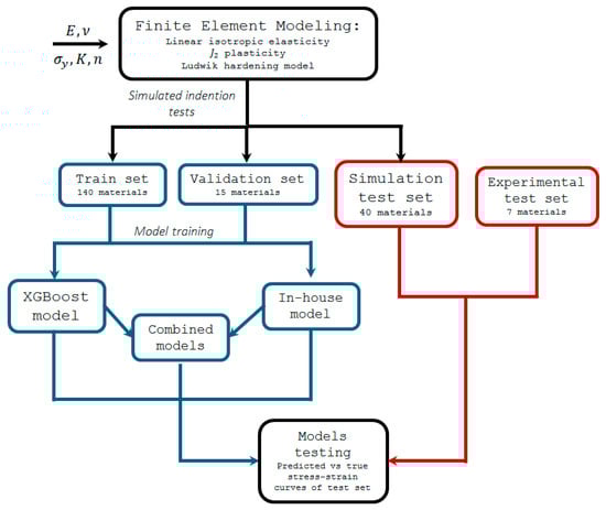
Figure 1.
A flow chart representing the methodology used in this research.
3. Database Creation for the Machine Learning Algorithm
Using finite element modeling, Brinell indentation tests were simulated for 205 sets of metallic materials with a distinct stress–strain response. In addition, a total of seven different materials on which physical indentation tests were performed were also used, as will be described later. In total, the force–displacement indentation response for 212 metallic materials was utilized in the current study. The database was then divided into three 150:15:47 train–validation–test subgroups or sets. The training set is used to construct the prediction models (i.e., identify missing functions/coefficients that define the prediction models). The validation set is used to tune hyper-parameters of the XGBoost-based models. The testing set is solely used to test every prediction model used in this work. All seven materials that were experimentally tested are only featured in the test set, while the rest of the test set includes simulated indentation tests.
In the finite element analysis, the materials were modeled as elastoplastic using the J2 yielding criterion with isotropic strain hardening. The elastic response was assumed to obey Hooke’s law, with Young’s modulus of 70 GPa and Poisson ratio of 0.33, known to be the moduli of aluminum alloys. However, this choice of parameters does not limit this work to aluminum alloys alone, as initial simulations verified that for different elastic moduli of common metal alloys, the variation in the indentation results is negligible.
The elastoplastic mechanical behavior was modeled using the Ludwik form:
where and are the equivalent stress and plastic strain, respectively, and are material parameters.
For the training set, a material database was constructed using different values of . The parameters chosen are shown in Table 1, resulting in a total number of 5 × 6 × 5 = 150 materials modeled. Eventually, relatively high-strength materials, which have either and , or and , were omitted from the materials database (ten materials in total, as each () combination has 5 different values of ). This is because their high strength did not produce valid indentation traces using the indentation forces chosen for this work.

Table 1.
Ludwig parameters chosen for the materials database.
For the validation and numerical test sets, the materials were constructed using uniformly distributed Ludwik coefficients, where the distribution’s extreme values are those of the training set. Experimental indentation data was obtained for seven materials. Two materials were taken directly from Richmond et al. [36], labeled as high and low-work hardening materials, respectively. The other five materials, which are Al1100, Al6061-T6, Al7075-T6, and brass and copper alloys, underwent experimental indentation using a Zwick µHU indentation machine, with indentation forces of 62.5, 153.065, 315.125, 625.25, and 1873.5 kgf. However, for some materials, not all forces were used, since some of them resulted in traces that were either too small or too big to visually determine their diameter. Specimens used for indentation had a thickness of at least 6 mm and a width and height of at least 10 times the indentation diameter. The five materials also underwent tensile tests using standard dogbone specimens. Testing was carried out using a Zwick/Roell 100 kN Allroundstanding (Ulm, Germany), with a loading rate of 1 [mm/min]. All specimens were loaded until fracture. All seven materials were used solely for testing the prediction models.
For every material set (train, validation, and test), every stress–strain curve was processed so that its yield point ( is defined as the conventional 0.2% yield point offset. This was conducted to better align with engineering interpretation conventions of stress–strain data.
An illustration of the curve processing is shown in Figure 2, and a graphical representation of the entire material database after processing can be seen in Figure 3. Note that every curve representation in this study is a true stress–strain curve. It should be noted that during the FE computations, the hardening curves of the materials were input directly into ABAQUS 2021 using the Ludwik equation parameters (different parameters for every material), which allow for generating the hardening curves automatically.
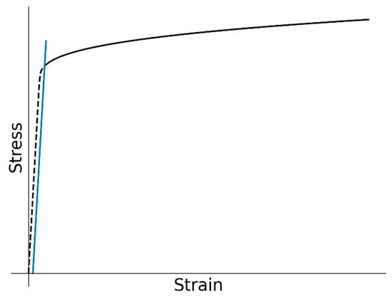
Figure 2.
Procedure for extracting the 0.2% yield point offset. The dashed curve is removed from the material curve.
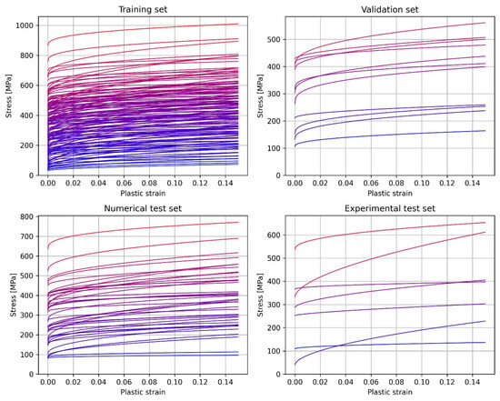
Figure 3.
A graphical representation of the stress–strain curves of all modeled materials.
Finite Element Modeling
Numerical indentation tests were carried out for all materials in the material database using the ABAQUS 2021 commercial software [37]. A 2D axisymmetric model of a specimen and an indenter was constructed, as can be seen in Figure 4. The specimen height was chosen to be 10 mm. This is in order to make sure that the height is at least ten times larger than the indentation depth, as is required according to the standard test method for the Brinell hardness [2]. The material model is the one described in the previous section. In contrast, the indenter was modeled as a rigid body, as the indenter’s material, tungsten carbide, has far larger yield stress than the tested materials. Penalty contact was enforced between the specimen and the indenter, with a friction coefficient of 0.2. This friction coefficient provided the best fit for the different experimentally tested materials. A two-step implicit scheme was chosen, such that the first step is applying load to the indenter, and the second step is unloading. The boundary conditions given for the model include a prescribed force for the indenter, a fixed bottom region of the specimen, and no displacement in the radial direction of the r = 0 plane for both parts. The force values chosen for the indenter are the same as those used for the experimental indentation tests. To minimize discretization error, the convergence of the solution with respect to mesh size must be verified [38,39]. A convergence test for the maximum equivalent stress, plastic strain, and internal energy was conducted, in which 21k degrees of freedom proved to be sufficient for achieving convergence, as can be seen in Figure 5. Finally, Figure 6 shows the equivalent stress and equivalent plastic strain fields, which were obtained while applying a load of 306 [N] and unloading. It can be seen that maximum deformation occurs near the end of the region of contact between the indenter and the specimen.
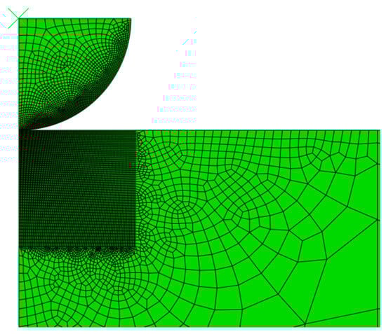
Figure 4.
A two-dimensional axisymmetric indentation model was used for indentation data generation.
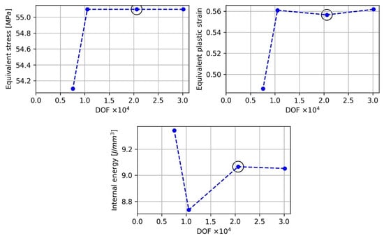
Figure 5.
Solution convergence tests for the indentation model, including equivalent stress, equivalent plastic strain, and internal energy. The number of DOFs used following verification is marked by a black circle.
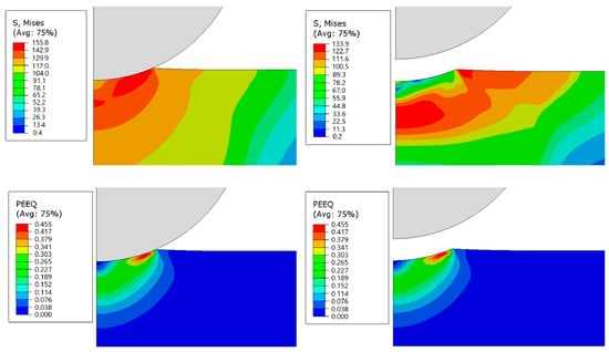
Figure 6.
Equivalent stress and equivalent plastic strain during load application and after unloading.
Calculating the indentation trace diameter was conducted by mimicking the procedure used in a real indentation test. For every numerical indentation test, a snapshot of a view normal to the specimen surface was taken. In the view, the r-coordinate of the end of the indentation contour was probed, being the indentation trace radius. This process is illustrated in Figure 7.
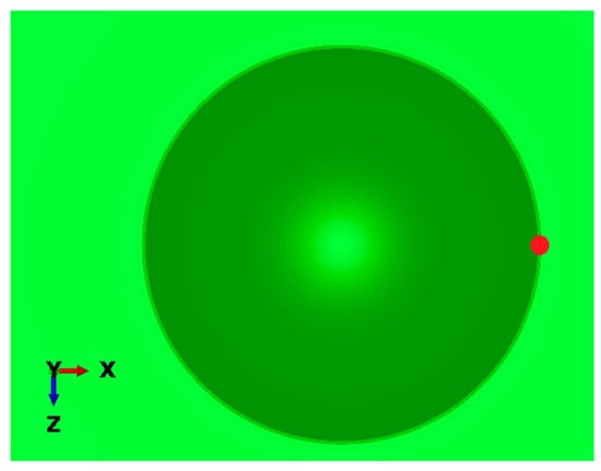
Figure 7.
Indentation trace generated in the numerical model, from which the indentation diameter was calculated. The probed point, acting as the trace radius, is indicated with a red circle.
After having established the numerical model and the means to obtain the indentation diameter, a validation test was conducted for the model by comparing experimental and numerical obtained indentation diameters for all five metals participating in the experimental section of this study under an applied load of 306 N. The test results, which are summarized in Table 2, suggest a good agreement between experimental and numerical results, with an average relative error of 4.7 ± 2.7%.
Table 2.
Comparison between indentation trace diameter obtained from the experiment and a numerical model for the five metals. The applied load was 306 [N].
4. Machine Learning Models
As mentioned in the methodology section, two main algorithms are utilized in this study. The first is an in-house statistical algorithm developed, and the second is known as the Extreme Gradient Boosting algorithm [35].
4.1. In-House Statistical Algorithm
Consider a typical Brinell indentation procedure featuring indentation force F, indenter diameter D, and trace diameter d. We define a pseudo equivalent plastic strain and pseudo equivalent stress measures for the indentation trace, termed as and , respectively. These pseudo measures are defined as follows:
The model’s core assumption is that both and are connected to the material’s true equivalent stress and plastic strain , and that this connection is true for all metallic materials. In other words, that there exist functions and , such that:
Identification of is conducted by exploring the constructed database in the previous section and trying to find correlations between both spaces (‘true’ and ‘hardness’), rather than by trying to devise analytical relations.
We first employ Meyer’s law [3] (Equation (6)) on the database.
where are material coefficients, which are obtained using linear regression on the term shown in Equation (7).
We then define a sub-function , which maps the pseudo equivalent stress to the true equivalent stress for a single pseudo strain value . i.e.,:
where:
By applying Meyer’s law from Equation (6):
Equation (9) outlines the scheme for finding and . Given a vector of desired strains . We search for every and its complementary , which produces a good correlation between the left and the right terms of Equation (9), for all of the materials in the train set. This is achieved by choosing a pair of (, and for that pair, plotting ( points for every material in the database (each material has a single ( for a given (, as the rest of the parameters () are material constants). Then, the value is held constant, and the is iteratively changed until the tightest possible spread (indicated by the value) of the data points is achieved.
Initially exploring the database, we find that some pairs do yield a good correlation for all materials in the training set. An example of this can be seen in Figure 8. A second-order polynomial fit was added to the scatter plot, which features a good fit, as indicated by the R2 value of 0.9952. As the pair shown in Figure 8 provides the tightest spread of data points, it also offers the best fit for all polynomial functions tested, up to a polynomial rank of 6.
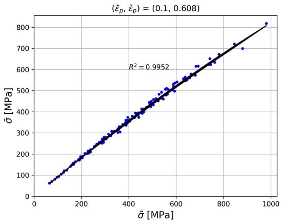
Figure 8.
Equivalent stress vs. hardness pseudo stress for every material in the database, together with a 2nd-order polynomial fit, for the (0.1, 0.608) pair of the equivalent strain and hardness pseudo strain.
Based on this finding, we assume that all sub-functions can be defined as 2nd-order polynomials:
4.2. Model Training
Training this model is essentially identifying and for a given database. From Equation (10), it seems that is a collection of 2nd-order polynomials. Therefore, an algorithm is utilized to find a 2nd-order polynomial fit, such as shown in Equation (10), for every strain point in the vector , in increments of 0.001. For every , the algorithm performs the following tasks:
Seeks for the pair , which gives the lowest sum of squared residuals of the polynomial fit.
Calculates the absolute error (L1 norm) of the curve for the best fit obtained (in other words, the prediction error of for a given ).
Applying it, both a pair and a curve were identified for every , thus defining and functions. Their 3D representations are shown in Figure 9 and Figure 10.
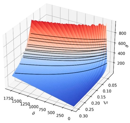
Figure 9.
A graphical representation of . Black lines represent a single material hardening curve.
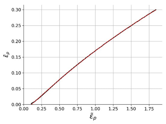
Figure 10.
A graphical representation of .
An error analysis was conducted by calculating the absolute error between each one of the graphs shown in Figure 3 and their prediction using the following formula:
where is the true flow curve, is the predicted flow curve, and is the number of the discrete points from which describe the flow curve. Figure 11 shows the absolute measured error as a function of the equivalent plastic strain, for all the materials in the training dataset. It seems that for (i.e., the yield point), the error renders the model unable to predict the yield stress. However, it rapidly drops with the increase of plastic deformation with showing the minimal error, which is around 9 MPa.
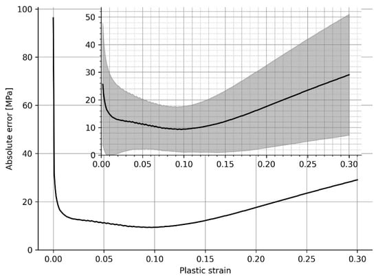
Figure 11.
Absolute error in predicting a material flow stress as a function of the plastic strain. The black line within the gray region represents the average and standard deviation of the calculated error for all materials used to train the model.
4.3. XGBoost Algorithm
XGBoost, an abbreviation for Extreme Gradient Boosting, belongs to the family of gradient boosting algorithms, which sequentially builds an ensemble of decision trees, with each subsequent learner focusing on the errors made by the previous ones. The following section briefly summarizes the XGBoost algorithm. A comprehensive overview can be found in Chen and Guestrin [35].
Given a training dataset , where represents features and denotes labels, the model aims to learn a model to predict . The objective function is as follows:
where is the loss function measuring the prediction deviation, is the regularization term penalizing model complexity, and is the number of weak learners. The regularization term is as follows:
where is the number of leaves in the tree, are leaf weights, and and are regularization parameters.
The algorithm utilizes gradient boosting, sequentially adding weak learners to minimize the objective function. Each iteration fits a tree to the negative gradient of the loss function with respect to the ensemble prediction:
The tree is then added to the prediction ensemble:
where is the learning rate.
4.4. Model Training and Validation
The XGBoost model was constructed using the XGBoost open-source library for Python [40]. An XGBRegressor instance was called with initial hyper-parameters and a root mean squared error as the evaluation metric. Using the GridSearchCV class from the scikit-learn library [41], both model training and hyper-parameter tuning (using a grid search) were conducted using the training and validation data shown in Section 3.
The parameter grid used for the grid search can be found in Table 3. Detailed explanations of each parameter can be found in the software documentation [40].
Table 3.
Parameter grid used for hyper-parameter tuning.
For the features selection for the database (i.e., the features chosen for each material, used by the model to predict the flow stress curve), initial tests proved that instead of using the raw force and diameter measurements from the indentation, using the Meyer coefficients and the calculated Brinell hardness yields better predictions. Therefore, these three were selected to be used as features.
Overall, the dataset for training, validation, and testing is a matrix , where i is the ith material, and j is either k, m, or the Brinell hardness measurement, which is calculated using Equation (1) [5].
5. Results
Using the two algorithms shown in the previous section, three different models were trained on the indentation database (that can also be seen in Figure 12):
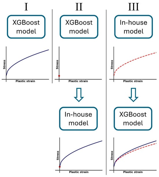
Figure 12.
Illustration of the three tested models.
- An XGBoost model for predicting the entire flow stress curve.
- An XGBoost model for predicting the yield stress, and an in-house model for predicting the hardening curve. This split between the two models stems from the in-house model’s inability to predict the yield stress, as shown in Figure 11.
- An in-house model’s initial prediction for the entire flow stress curve, fed as an input to a subsequent XGBoost model for predicting the entire flow stress curve. This is performed in order to check whether the XGBoost model’s performance can be improved using the in-house model’s prediction (without the yield stress).
For each model, the training phase was conducted as laid out in sections 0 and 0 for the in-house and XGBoost algorithms, respectively.
Prediction Results and Discussion
Due to the larger absolute error for plastic strains greater than 0.15 presented in Figure 8, it is more useful to limit the model to predictions in the range of [0, 0.15] plastic strain. It should be noted that the uniform elongation of many metallic materials typically falls within the range of 0–15% true plastic strain. Some examples include but are not limited to, Al6061-T6, Al7075-T6, and Al2024-T351. This makes the range of [0, 0.15] examined in this study highly applicable for many engineering applications. Nevertheless, the methodology presented in this study can be applied to materials with greater ductility, provided that the database used for training the model is expanded to include materials with greater uniform elongation. In any case, it is important to understand that the model cannot predict the stress–strain response past the point of ultimate stress.
Predictions using the in-house model utilized 31 strain points equally dividing the strain range—30 points for the hardening curve and 1 yield point. Predictions using the XGBoost model utilized 6 strain points—5 for the hardening curve and 1 yield point. Increasing the number of points in the XGBoost model comes at the expense of higher computation time with roughly the same prediction error.
Prediction error was determined using two metrics:
- The relative error defined as follows:
- The root mean squared error defined as follows:
A summary comparison of the prediction errors of all four models can be found in Figure 13 for both the yield stress and the entire flow stress curve predictions. The bar graphs represent the average error (relative and root mean squared) among all tested materials, while the error bars represent the standard deviation of the average values.
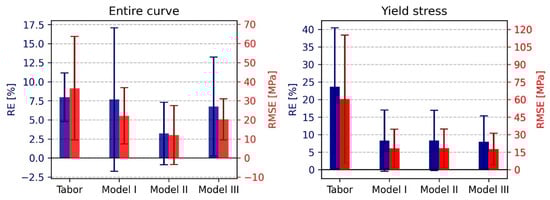
Figure 13.
Relative error and root mean squared error comparison between all four models. (Left) flow curve. (Right) yield stress.
Comparing the yield stress prediction performance, it can be seen that models I through III outperform the Tabor model, which has a relative error of about 25%. Furthermore, all these three models roughly share the same prediction error. This makes sense since all of them are essentially using the XGBoost algorithm for the yield stress predictions.
- Performance based on the material’s yield stress:
Looking at the models’ performance for the entire curve prediction, it seems that model II features the lowest relative and RMS errors. The Tabor model manages to score the same RE as Models I and III, albeit with a higher RMSE compared to them. This suggests that Tabor’s RMSE is proportional to the ‘height’ of the flow curve. In contrast, the rest of the models’ RMSE is more randomly distributed (so that cases of high RMSE for low-strength materials heavily increase the RE). To further investigate this matter, the performance of both the Tabor model and Model II was evaluated based on the yield stress of the tested material. The results of this analysis, presented in Figure 14 and Figure 15, show that the RMSE of the Tabor model increases for materials exhibiting a higher strength. This implies that the higher the strength, the worse the stress–strain prediction using Tabor’s model. In contrast, Model II features a relatively similar RMSE regardless of the material’s strength.
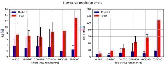
Figure 14.
Flow curve prediction errors, based on the yield stress of the predicted material. (Left) relative error. (Right) root mean squared error.
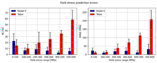
Figure 15.
Yield stress prediction errors, based on the yield stress of the predicted material. (Left) relative error. (Right) root mean squared error.
Another interesting finding is that for yield stress prediction for materials with a yield stress in the range of up to 100 MPa, it seems that the Tabor model outperforms Model II, both in RMSE and RE metrics. Because of this, Model II is updated to use the Tabor model for yield stress prediction if the initial prediction of the model suggests a yield stress lower than 100 MPa.
- Performance based on the maximum plastic strain to be predicted:
Another matter to be inspected is how the error metrics distribute as a function of the maximum plastic strain. Recall that until now, all flow curve predictions were performed with the strain range . Since the prediction error for the yield stress is different than that of the entire flow curve for all tested models, it is safe to assume that there is a variation in the error as the flow curve progresses in plastic strain. In other words, that the prediction error for the strain range is dependent on the chosen .
Investigating the matter, predictions were carried out for ( is essentially yield stress prediction), for Model II and the Tabor model (the reference model), with the results shown in Figure 16. Model II manages to keep its relative error below 5% throughout the inspected strain range, keeping both errors constant from 0.05 plastic strain onwards. In contrast, the Tabor model exhibits a relative error higher than 10% for plastic strain values lower than 0.1. The decrease in error as the plastic strain increases is not surprising since the Tabor model assumes fully developed plastic deformation beneath the indenter [4], which is not the case at the onset of yielding. This is also why the Tabor model shows high prediction errors for materials exhibiting higher yield stress—since the plastic strain under the indenter is not fully developed due to the higher elastic deformation.
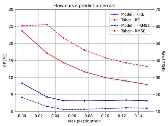
Figure 16.
RE and RMSE as a function of the maximum plastic strain chosen for the flow curve prediction.
- Prediction of materials used in real indentation tests:
Figure 17 and Table 4 show a comparison between Model I-generated curves and true curves of the experimentally tested materials (refer to Section 3). The true curves of the experimentally tested materials were obtained using classical uniaxial tensile experiments (some of the materials had their curve extrapolated using their Ludwik parameters, as their uniform elongation was lower than 0.15). Note that the two materials taken from Richmond et al. [36] do not feature a yield stress, as it was not reported in the original paper.
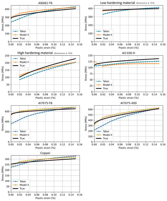
Figure 17.
Model II-generated stress–strain curves of the experimentally tested materials compared to true curves (Data for low and high hardening material taken from [36]).
Table 4.
Relative and root mean squared prediction errors of Model II, for the experimentally tested materials.
Overall, a good fit is seen for all materials, with only the Al1100-H featuring a relative error higher than 10%. This comparison suggests that the proposed model manages to predict the flow stress curve from real indentation tests as well.
6. Summary and Conclusions
In this study, a data-driven approach that leverages machine learning and finite element analysis was used to construct a model that predicts the stress–plastic strain curve of metallic materials from a minimum of two indentation tests. The final model, termed ‘Brilearn’, consists of several sub-models, which are as follows:
- A Tabor model for predicting the yield stress of metals with a yield stress lower than 100 MPa.
- An XGBoost model for predicting the yield stress of metals with a yield stress higher than 100 MPa.
- An in-house developed model for predicting the hardening curve.
The model features error predictions of 8.4 ± 8.5% for the yield stress and 3.2 ± 4% for a complete curve ranging from to .
To practically use the ‘Brilearn’, first download it from the online repository (see data availability statement).
Then, the following steps are taken:
- Conduct Brinell hardness tests with different values of indentation forces. A minimum of two tests with different forces is required, although more test data will ensure more accurate results.
- Convert the force and trace diameter data from the hardness tests to the pseudo stress and pseudo strain values using Equation (4).
- Identify the Meyer coefficient of the material using the values calculated from Equation (4). Note that the model contains a tool for automatically identifying these coefficients (see the data availability statement for an online repository where the ML-model and tools can be found).
- Input the Meyer coefficients and the Brinell hardness values measured in the ML-model to generate the material hardening curve.
The model is especially suited for the determination of the stress–plastic strain curves for components in service since only two simple indentation tests are required.
Author Contributions
Conceptualization, N.R. and E.P.; methodology, N.R.; formal analysis, N.R.; resources, E.P.; writing—original draft preparation, N.R.; writing—review and editing, E.P.; funding acquisition, E.P. All authors have read and agreed to the published version of the manuscript.
Funding
This research received no external funding.
Data Availability Statement
The Brilearn model and code, along with the data generated for its generation, is available in the following online repository: Rom. N, Priel. E, “Brilearn” GitHub, April 2024. [Online]. https://github.com/NitzanRom/Brilearn (accessed on 1 January 2025).
Conflicts of Interest
The authors declare no conflicts of interest.
References
- Brinell, J.A. SaÈtt att bestaÈmma kroppars haÊrdhet jaÈmte naÊgra tillampningar af detsamma. Teknisk Tidskrift 1900, 30, 69–87. [Google Scholar]
- ASTM E10-15; Standard Test Method for Brinell Hardness of Metallic Materials. ASTM International: West Conshohocken, PA, USA, 2015.
- Meyer, E.; Ver, Z. Contribution to the knowledge of hardness and hardness testing. Z. Vereines Dtsch. Ingenieure 1908, 52, 645–654. [Google Scholar]
- Tabor, D. A simple theory of static and dynamic hardness. Proc. R. Soc. Lond. Ser. A Math. Phys. Sci. 1948, 192, 247–274. [Google Scholar]
- Hill, R.; Storakers, B.; Zdunek, A.B. A theoretical study of the Brinell hardness test. Proc. R. Soc. Lond. A 1989, 423, 301–330. [Google Scholar]
- Oliver, W.C.; Pharr, G.M. An improved technique for determining hardness and elastic modulus using load and displacement sensing indentation experiments. J. Mater. Res. 1992, 7, 1564–1583. [Google Scholar] [CrossRef]
- Nix, W.D.; Dao, H. Indentation size effects in crystalline materials: A law for strain gradient plasticity. J. Mech. Phys. Solids 1998, 46, 411–425. [Google Scholar] [CrossRef]
- Bîrleanu, C.; Pustan, M.; Șerdean, F.; Merie, V. AFM Nanotribomechanical Characterization of Thin Films for MEMS Applications. Micromachines 2022, 13, 23. [Google Scholar] [CrossRef]
- Zak, S.; Trost, C.O.; Kreiml, P.; Cordill, M.J. Accurate measurement of thin film mechanical properties using nanoindentation. J. Mater. Res. 2022, 37, 1373–1389. [Google Scholar] [CrossRef]
- Zak, S. Controlling strain localization in thin films with nanoindenter tip sharpness. Sci. Rep. 2024, 14, 25500. [Google Scholar] [CrossRef] [PubMed]
- Khalfallah, A.; Khalfallah, A.; Benzarti, Z. Identification of Elastoplastic Constitutive Model of GaN Thin Films Using Instrumented Nanoindentation and Machine Learning Technique. Coatings 2024, 14, 683. [Google Scholar] [CrossRef]
- Soowan, P.; Karuppasamy, P.M.; Giyeol, H.; Hyungyil, L. Deep learning based nanoindentation method for evaluating mechanical properties of polymers. Int. J. Mech. Sci. 2023, 246, 108162. [Google Scholar]
- Niu, J.; Miao, B.; Guo, J.; Ding, Z.; He, Y.; Chi, Z.; Wang, F.; Ma, X. Leveraging Deep Neural Networks for Estimating Vickers Hardness from Nanoindentation Hardness. Materials 2024, 17, 148. [Google Scholar] [CrossRef] [PubMed]
- Chen, T.T.; Watanabe, I. Data-driven estimation of plastic properties in work-hardening model combining power-law and linear hardening using instrumented indentation test. Sci. Technol. Adv. Mater. Methods 2022, 2, 416–424. [Google Scholar] [CrossRef]
- Dao, M.; Chollacoop, N.; Van Vliet, K.J.; Venkatesh, T.A.; Suresh, S. Computational modeling of the forward and reverse problems in instrumented sharp indentation. Acta Mater. 2001, 49, 3899–3918. [Google Scholar] [CrossRef]
- Bucaille, J.L.; Stauss, S.; Felder, E.; Michler, J. Determination of plastic properties of metals by instrumented indentation using different sharp indenters. Acta Mater. 2003, 51, 1663–1678. [Google Scholar] [CrossRef]
- Goto, K.; Watanabe, I.; Ohmura, T. Inverse estimation approach for elastoplastic properties using the load-displacement curve and pile-up topography of a single Berkovich indentation. Mater. Des. 2020, 194, 108925. [Google Scholar] [CrossRef]
- Kang, J.J.; Becker, A.A.; Sun, W. Determining elastic–plastic properties from indentation data obtained from finite element simulations and experimental results. Int. J. Mech. Sci. 2012, 62, 34–46. [Google Scholar] [CrossRef]
- Fernandez-Zelaia, P.; Joseph, V.R.; Kalidindi, S.R.; Melkote, S.N. Estimating mechanical properties from spherical indentation using Bayesian approaches. Mater. Des. 2018, 147, 92–105. [Google Scholar] [CrossRef]
- Lu, L.; Dao, M.; Kumar, P.; Ramamurty, U.; Karniadakis, G.E.; Suresh, S. Extraction of mechanical properties of materials through deep learning from instrumented indentation. Proc. Natl. Acad. Sci. USA 2020, 117, 7052–7062. [Google Scholar] [CrossRef]
- Karuppasamy, P.M. Physics-informed neural networks for spherical indentation problems. Mater. Des. 2023, 236, 112494. [Google Scholar]
- Haj-Ali, R.; Kim, H.K.; Koh, S.W.; Saxena, A.; Tummala, R. Nonlinear constitutive models from nanoindentation tests using artificial neural networks. Int. J. Plast. 2008, 24, 371–396. [Google Scholar] [CrossRef]
- Ma, Q.P.; Basterrech, S.; Halama, R.; Omacht, D.; Měsíček, J.; Hajnyš, J.; Platoš, J.; Petrů, J. Application of instrumented indentation test and neural networks to determine the constitutive model of in-situ austenitic strainless steel components. Arch. Civ. Mech. Eng. 2024, 24, 129. [Google Scholar] [CrossRef]
- Yongju, K. Novel deep learning approach for practical applications of indentation. Mater. Today Adv. 2022, 13, 100207. [Google Scholar]
- Dieter, G.E. Mechanical Metallurgy; McGraw-Hill Book Company: New York, NY, USA, 1961. [Google Scholar]
- Jayaraman, S.; Hahn, G.T.; Oliver, W.C.; Rubin, C.A.; Bastias, P.C. Determination of the monotonic stress-strain curve of hard materials from ultra-low-load indentation tests. Int. J. Solids Struct. 1998, 35, 365–381. [Google Scholar] [CrossRef]
- DiCarlo, A.; Yang, H.T.Y.; Chandrasekar, S. Prediction of stress-strain relation using cone indentation: Effect of friction. Int. J. Numer. Methods Eng. 2004, 60, 661–674. [Google Scholar] [CrossRef]
- Liu, X.; Peng, Q.; Pan, S.; Du, J.; Yang, S.; Han, J.; Lu, Y.; Yu, J.; Wang, C. Machine Learning Assisted Prediction of Microstructures and Young’s Modulus of Biomedical Multi-Component β-Ti Alloys. Metals 2022, 12, 796. [Google Scholar] [CrossRef]
- Liu, Z.; Zhang, H.; Zhang, S.; Cheng, J.; He, Y.; Zhou, G.; Liu, J.; Song, S.; Chen, L. A machine learning method approach for designing novel high strength and plasticity metastable β titanium alloys. Prog. Nat. Sci. Mater. Int. 2024. [Google Scholar] [CrossRef]
- Churyumov, A.Y.; Kazakova, A.A. Prediction of True Stress at Hot Deformation of High Manganese Steel by Artificial Neural Network Modeling. Materials 2023, 16, 1083. [Google Scholar] [CrossRef] [PubMed]
- Jeong, J.; Hong, D.; Yim, C. Deep Learning to Predict Deterioration Region of Hot Ductility in High-Mn Steel by Using the Relationship between RA Behavior and Time-Temperature-Precipitation. Metals 2022, 12, 1689. [Google Scholar] [CrossRef]
- Vivanco-Benavides, L.E.; Martínez-González, C.L.; Mercado-Zúñiga, C.; Torres-Torres, C. Machine learning and materials informatics approaches in the analysis of physical properties of carbon nanotubes: A review. Comput. Mater. Sci. 2022, 201, 110939. [Google Scholar] [CrossRef]
- Juan, Y.; Dai, Y.; Yang, Y.; Zhang, J. Accelerating materials discovery using machine learning. J. Mater. Sci. Technol. 2021, 79, 178–190. [Google Scholar] [CrossRef]
- Pan, S.; Wang, Y.; Yu, J.; Yang, M.; Zhang, Y.; Wei, H.; Chen, Y.; Wu, J.; Han, J.; Wang, C.; et al. Accelerated discovery of high-performance Cu-Ni-Co-Si alloys through machine learning. Mater. Des. 2021, 209, 109929. [Google Scholar] [CrossRef]
- Chet, T.; Guestrin, C. XGBoost: A Scalable Tree Boosting System. In Proceedings of the 22nd ACM SIGKDD International Conference on Knowledge Discovery and Data Mining, San Francisco, CA, USA, 13–17 August 2016; pp. 785–794. [Google Scholar]
- Richmond, O.; Morrison, H.; Devenpeck, M. Sphere indentation with application to the Brinell hardness test. Int. J. Mech. Sci. 1974, 16, 75–82. [Google Scholar] [CrossRef]
- ABAQUS, 2022; Dassault Systèmes: Providence, RI, USA, 2022.
- Rom, N.; Bortman, J.; Priel, E. Predicting ductile failure of aluminum components under general loading conditions: Computational implementation, model verification and experimental validation. Int. J. Solids Struct. 2023, 275, 112295. [Google Scholar] [CrossRef]
- Priel, E.; Mittelman, B.; Trabelsi, N.; Cohen, Y.; Koptiar, Y.; Oadan, R. A computational study of equal channel angular pressing of molybdenum validated by experiments. J. Mater. Process. Technol. 2019, 264, 469–485. [Google Scholar] [CrossRef]
- XGBoost Developers. XGBoost Documentation. Version 2.0.3. December 2023. Available online: https://xgboost.readthedocs.io/en/stable/index.html (accessed on 20 May 2024).
- Pedregosa, F.; Varoquaux, G.; Gramfort, A.; Michel, V.; Thirion, B.; Grisel, O.; Blondel, M.; Prettenhofer, P.; Weiss, R.; Dubourg, V.; et al. Scikit-learn: Machine learning in Python. J. Mach. Learn. Res. 2011, 12, 2825–2830. [Google Scholar]
Disclaimer/Publisher’s Note: The statements, opinions and data contained in all publications are solely those of the individual author(s) and contributor(s) and not of MDPI and/or the editor(s). MDPI and/or the editor(s) disclaim responsibility for any injury to people or property resulting from any ideas, methods, instructions or products referred to in the content. |
© 2025 by the authors. Licensee MDPI, Basel, Switzerland. This article is an open access article distributed under the terms and conditions of the Creative Commons Attribution (CC BY) license (https://creativecommons.org/licenses/by/4.0/).