Establishment of an Improved Elman Neural Network Model for Predicting the Corrosion Rate of 3C Steel in Marine Environment and Analysis of the Factors Affecting Model Accuracy

Abstract

3C steel is a kind of steel commonly used in marine engineering, which will suffer different degrees of corrosion in the marine environment. In the marine environment, there is a complex nonlinear relationship between the corrosion rate and seawater environmental parameters. Based on the experimental data of corrosion rates of 3C steel in different seawater environments, an improved Elman neural network model was established by using the whale optimization algorithm. The corrosion rates of 3C steel in different seawater environments were predicted, and the influences of the number of hidden layer nodes, the population sizes, and the number of iterations on the prediction results of the improved model were analyzed. The results show that the prediction results of the improved Elman neural network model are in good agreement with the experimental results; the average relative error and the root mean square error are 1.0564% and 0.195, respectively. With the increase in the number of hidden layer nodes and the population sizes, the average relative errors of the predicted results decrease first and then increase. With the increase in the number of iterations, the average relative errors of the predicted results decrease first, then increase, and finally decrease. The improved Elman neural network model has the advantage of high prediction accuracy and can be applied to the prediction of the corrosion rate of 3C steel in the marine environment.

1. Introduction

In the marine environment, seawater is a highly corrosive natural electrolyte that causes many materials to suffer different degrees of corrosion. The corrosion of materials in the marine environment will not only cause huge economic losses but also have a great impact on the safe operation of equipment [1,2,3]. 3C steel is a kind of carbon steel that is widely used in chemical products, petroleum production, refinery, pipelines, etc. [4]. 3C steel has excellent working performance (such as physical, chemical, and mechanical properties) and process characteristics (such as welding performance, toughness, and cutting performance) [5].

In the complex marine environment, the research on the corrosion rate of 3C steel has always been an important content in the field of corrosion. For the study of the corrosion rate, relevant testing techniques can be used. Zou et al. estimated the corrosion rate of mild steel in long-term immersion by using electrochemical and weight-loss methods. The authors pointed out that the results of the electrochemical estimation method are consistent with those of the weight-loss method during the initial immersion period, but there is a big deviation between the results obtained by the two methods after long-term immersion [6]. Ferry et al. measured the corrosion rate of the coupon plate surface by electrochemical impedance spectroscopy and analyzed the influence of seawater velocity on the corrosion rate of mild steel. The results showed that the corrosion rate increases with the increase in seawater velocity [2]. Wang et al. used electrochemical, artificial neural network, and database methods to study the off-site corrosion behavior of marine engineering steels. The experimental results showed that the influence of temperature and salinity on the corrosion rate of 3C steel is complex, and the corrosion rate linearly increases with the increase in the oxygen content [7].

In addition to using relevant experimental testing technology to study the corrosion rate of steel, the method of establishing models can also be used. Compared with the experimental test method, it is faster and simpler to predict the corrosion rate of steel by establishing the models [8]. However, there are many factors affecting steel corrosion in the seawater environment (temperature, dissolved oxygen content, salinity, etc.), which makes it difficult to study the relationship between seawater environmental factors and the corrosion rate and increases the difficulty of establishing mathematical models [1,9].

In recent years, with the continuous development of machine-learning theory, many scholars have applied machine-learning methods to predict the corrosion rate. Paul et al. established an ANN model for predicting the corrosion rate. The authors pointed out that the model can be used to predict the corrosion rate of some practical systems [1]. Kamrunnahar et al. introduced the idea of a supervised neural network into the prediction of the corrosion behavior of metal alloys and achieved good prediction results [10]. Based on the dynamic corrosion experiment, Chen et al. used an alternating conditional expectation algorithm to establish a prediction model of the corrosion rate of carbon steel. The authors pointed out that the model can accurately predict the corrosion rate at different temperatures, pH values, and ion concentrations, and the results are more accurate than those of the BP neural network and support vector regression [11]. Although a neural network has strong advantages in the field of prediction, the traditional artificial neural network has the disadvantage of easily falling into the local minimum value [12].

In order to overcome the shortcomings of traditional neural network models, many scholars have adopted relevant improvement methods and achieved good prediction results [4,13,14,15,16]. Among these improvement methods, some scholars have used the imperial competitive algorithm, the genetic algorithm, and the adaptive multilayer particle swarm to improve the ANN model and predicted the corrosion behavior of materials based on the improved model. For the ANN model, the network topology and the algorithm to train the set of synaptic weights have a great influence on the performance of the model. In addition, the genetic algorithm has the disadvantages of high computational complexity and may fall into the local optimal solution (with a certain degree of randomness) in the application process. For the imperialist competitive algorithm, it still faces problems such as rapid decline in population diversity, easy premature convergence, and low solution accuracy.

In the process of neural network prediction, the Elman neural network is a typical dynamic artificial neural network with excellent nonlinear fitting ability and certain local memory function [17]. Although the Elman neural network has strong advantages, there are still some shortcomings (the training speed is slow and easy to fall into a local minimum value) [18]. Therefore, how to improve the prediction performance of the Elman network model is still an important research content.

The whale optimization algorithm was introduced by Mirjalili and Lewis to solve optimization problems [19]. The algorithm can overcome the problems of slow convergence speed and local minimum of the neural network and can estimate the neighborhood space of the global optimal solution. Therefore, it is an efficient algorithm to solve the optimization problem [20].

In the process of applying machine-learning algorithms to predict the corrosion behavior of materials, researchers have adopted relevant improved algorithms to improve the ANN model. Although the whale optimization algorithm has strong advantages, there are still few reports on the establishment of an Elman neural network model based on the whale optimization algorithm to predict the corrosion rate of steel. For this reason, this article established an improved Elman neural network model based on the whale optimization algorithm to predict the corrosion rate of 3C steel, and the influences of different factors on the prediction accuracy of the improved model were discussed. The improved model proposed in this paper provides a new idea for the accurate prediction of the corrosion rate of 3C steel and has the advantages of convenient application and saving of financial resources. In addition, the improved neural network model has strong nonlinear mapping ability and has a strong application value.

2. Basic Principles of Elman Neural Network and Whale Optimization Algorithm

2.1. Elman Neural Network (ENN)

The Elman neural network consists of an input layer, a hidden layer, a context layer, and an output layer. The specific structure diagram of the Elman neural network has been given in reference [17], and readers can refer to it by themselves.

The expressions of the Elman neural network structure are as follows [17,21]:

$$y\left(t\right)=g(w_{3}x(t))$$

(1)

$$x\left(t\right)=f(w_1(u(t-1))+w_2{x}_c(t))$$

(2)

$$x_c\left(t\right)=x(t-1)$$

(3)

where y(t) is the output of the neural network. w₃ is the connection weight from the hidden layer to the output layer. x(t) is the output of the hidden layer at time t. g is the transfer function of the output layer. f is the transfer function of the hidden layer. w₁ is the connection weight from the input layer to the hidden layer. w₂ is the connection weight from the context layer to the hidden layer. u(t − 1) is the input of the neural network at time t. x_c(t) is the input from the hidden layer to the context layer.

The operating principle of the Elman neural network structure is as follows:

The data information is input through the input layer, and it is transmitted to the hidden layer with linear and nonlinear excitation functions. The context layer is used to remember the output value of the neural unit at the previous moment, then its delay and memory effects create a correlation between the output and input of the hidden layer. Finally, weighted processing is performed in the output layer [18].

2.2. Whale Optimization Algorithm (WOA)

The WOA optimization process starts from randomly initializing the population, and the whole process is divided into three stages (encircling prey, bubble-net attacking, and randomly searching for prey) [22]. The specific descriptions of each stage are as follows [22,23,24,25,26,27,28,29].

2.2.1. Encircling Prey

Suppose that the candidate solution with the best fitness in the current population is the position of the prey or the position of the approaching target prey, and the other search individuals of the population update their positions according to the current optimal candidate solution. This process can be expressed by Formulas (4) and (5):

$$\mathrm{D}=\left|\mathrm{C}·{\mathrm{X}}^{*}(t)-\mathrm{X}(t)\right|$$

(4)

$$\mathrm{X}(t+1)={\mathrm{X}}^{*}(t)-\mathrm{A}·\mathrm{D}$$

(5)

where t is the number of iterations. ${\mathrm{X}}^{*}(t)$ is the position of the optimal solution for the current population. $\mathrm{X}(t)$ is the current position of the whale. D is the distance between the current whale position and ${\mathrm{X}}^{*}(t)$. A and C are coefficient vectors, and the calculation formulas are as follows:

$$a=2-{\displaystyle \frac{2t}{t_{\max }}}$$

(6)

$$\mathrm{A}=2a·r-a$$

(7)

$$\mathrm{C}=2·r$$

(8)

where r is a random number between 0 and 1. a is a control parameter that can be linearly reduced from 2 to 0 during the iteration process. $t_{\max }$ is the maximum iteration number.

2.2.2. Bubble-Net Attacking Approach

There are two strategies: shrinking encircling and spiral updating position.

• Shrinking encircling mechanism: this behavior is achieved by adjusting the a value in Formula (7).
• Spiral updating position: the distance between the whale and the prey is first calculated, and then the spiral motion of the whale is imitated to hunt the prey. The specific formulas are as follows:

  $${\mathrm{D}}^{\prime }=\left|{\mathrm{X}}^{*}(t)-\mathrm{X}(t)\right|$$

  (9)

  $$\mathrm{X}(t+1)={\mathrm{D}}^{\prime }·{\mathrm{e}}^{bl}·\cos (2\pi l)+{\mathrm{X}}^{*}(t)$$

  (10)

  where b is a constant coefficient that characterizes the spiral shape. l is a random number within [−1,1].

In the optimization process, whales need to shrink their encirclement range and simultaneously surround their prey along a spiral path, and the probability of these two ways is equal. The specific expression is as follows:

$$\mathrm{X}(t+1)=\left\{\begin{array}{ll}{\mathrm{X}}^{*}(t)-\mathrm{A}·\mathrm{D}& \mathrm{if}\mathrm{p}<0.5\\ {\mathrm{D}}^{\prime }·{\mathrm{e}}^{bl}·\cos (2\pi l)+{\mathrm{X}}^{*}(t)& \mathrm{if}\mathrm{p}\ge 0.5\end{array}\right.$$

(11)

where p is the probability factor within [0,1].

2.2.3. Randomly Search for Prey

The global search method is used to search for prey, and this process updates the position by randomly selecting search individuals. The specific formulas are as follows:

$$\mathrm{D}=\left|\mathrm{C}·{\mathrm{X}}_{\mathrm{rand}}(t)-\mathrm{X}(t)\right|$$

(12)

$$\mathrm{X}(t+1)={\mathrm{X}}_{\mathrm{rand}}(t)-\mathrm{A}·\mathrm{D}$$

(13)

where ${\mathrm{X}}_{\mathrm{rand}}(t)$ is the position (random selection) of the whale in the current population.

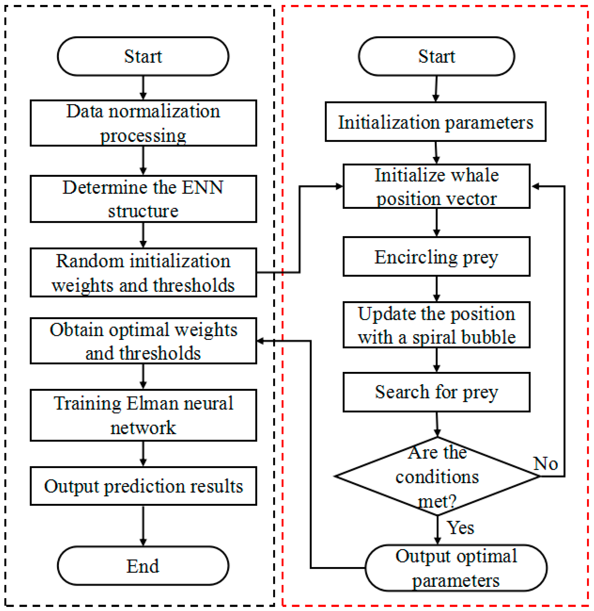
3. The Prediction Steps of Improved Elman Neural Network

According to the steps of Figure 1 and combined with Python programming language (version number: 3.12.5), the corrosion rates under different influencing factors were predicted.

Figure 1. The prediction flow chart of improved Elman neural network model.

The specific steps are as follows:

Step 1: On the basis of normalizing the measured data of the corrosion rate, the parameters of a traditional Elman neural network model are initialized, and the numbers of the input layer, the hidden layer, and the output layer are determined. The weights and thresholds initialized by the traditional Elman neural network are used as the initial position vector of the whale optimization algorithm, and the initial parameters of the whale optimization algorithm are set (including the population size, the number of iterations, the problem dimension, etc.).

Step 2: The population fitness values are calculated. The fitness function (Formula (14)) is constructed to determine the optimal solution in the overall optimization process.

$$fitness={\displaystyle \frac{1}{n}}{{\displaystyle \sum _{i=1}^n\left(d_{fi}-d_{vi}\right)}}^2$$

(14)

where n is the number of training samples. d_fi is the model output value of the i-th training sample. d_vi is the actual value of the i-th training sample.

Step 3: The current position of each whale individual is updated by the whale optimization algorithm, and the corresponding fitness value of each whale individual at this position is obtained. In the iterative process, the whale individual position corresponding to the optimal fitness of each iteration is recorded. If the optimal fitness value of the whale individual at the current position is better than the historical optimal fitness value, the position is updated. Otherwise, it is not updated.

Step 4: The termination condition is determined, and the optimal parameters are generated. If the current number of iterations is fewer than the total number of iterations, then steps 2 and 3 are performed. Otherwise, the optimal parameters are output.

Step 5: The optimal solution (the optimal weight values and threshold values) is assigned to the Elman neural network model, then an improved Elman neural network model is obtained through matrix reconstruction, and the corrosion rate of 3C steel is predicted.

4. The Prediction Results of Corrosion Rate of 3C Steel in Marine Environment

The authors of reference [30] took the experimental data of the corrosion rate of 3C steel under different seawater environmental factors (a total of 26 sets of data) as the research object and established a prediction model of the corrosion rate based on an extreme learning machine.

In this article, 21 sets of training sample data (as shown in Table 1) were used to establish the ENN model and the WOA-ENN model, and the remaining 5 sets of data (as shown in Table 2) were used as prediction samples for model validation.

Table 1. Training samples.

Num	Temperature/°C	Dissolved Oxygen Content/(mg·mL−1)	Salinity /‰	pH	Redox Potential/mV	Corrosion Rate/(μA·cm−2)
1	25.9000	6.7100	30.1000	5.1000	378.0000	16.4000
2	27.9000	6.1800	31.5000	7.0000	363.0000	15.5700
3	28.0000	5.0500	31.4000	9.2000	240.0000	13.2400
4	27.3200	3.2100	29.3100	8.2000	281.0000	12.9100
5	27.8700	6.5500	31.6800	7.2000	356.0000	14.0600
6	24.2700	0.8000	32.5600	8.1000	171.0000	3.6059
7	27.4500	2.6000	35.3700	7.9600	287.0000	7.9385
8	27.2300	4.2000	31.9400	7.8900	289.0000	9.6304
9	28.7500	6.8000	32.2200	8.0000	340.0000	11.4258
10	28.5200	8.4000	32.1000	8.0100	345.0000	12.5193
11	23.9500	7.6100	9.1700	8.0400	231.0000	10.9382
12	24.7300	6.0600	17.3300	7.8800	321.0000	11.4456
13	24.5100	7.0200	32.0000	8.1600	308.0000	12.5497
14	25.5700	6.7000	32.1900	8.0900	325.0000	11.8715
15	31.1600	4.3800	33.2100	7.9400	242.0000	8.9236
16	23.6500	6.5100	41.3400	7.6700	245.0000	8.4016
17	16.7400	7.1100	33.5500	8.2500	178.0000	10.8502
18	28.4500	9.9000	31.9500	7.9300	309.0000	22.6363
19	24.0000	7.9500	30.2000	8.1000	324.0000	13.6500
20	27.4800	5.9000	32.3900	7.8300	331.0000	10.5783
21	29.3500	6.0900	29.0000	6.3000	400.0000	16.9000

Table 2. Prediction samples.

Num	Temperature/°C	Dissolved Oxygen Content/(mg·mL−1)	Salinity/‰	pH	Redox Potential/mV	Corrosion Rate/(μA·cm−2)
1	29.3700	6.8200	30.1200	6.2000	414.0000	17.1100
2	28.2700	6.9800	28.2000	6.6000	384.0000	15.4700
3	21.1100	6.0300	33.4400	8.0300	295.0000	11.4479
4	30.7000	7.1500	31.7400	6.5000	401.0000	16.2800
5	24.6000	7.5200	24.4200	7.5700	210.0000	11.8285

Before determining the structure of the Elman neural network, it is necessary to determine the number of hidden layer nodes; the empirical formula used in this article is shown in Equation (15) [31].

$$H=\sqrt{m+n}+a$$

(15)

where m is the number of input layer nodes. n is the number of output layer nodes. a is an integer between 1 and 10.

Based on Equation (15), the different hidden layer nodes can be obtained. In order to determine the optimal number of hidden layer nodes, this paper calculates the mean squared errors of training samples under a different number of hidden layer nodes, and the results are shown in Table 3.

Table 3. Mean square errors of training samples under different numbers of hidden layer nodes.

Number	MSE
3	0.1831
4	0.1340
5	0.3429
6	0.0844
7	0.4134
8	0.1481
9	0.0955
10	0.1451
11	0.2125
12	0.1321

It can be seen from Table 3 that the mean squared error of training samples is the smallest when the number of hidden layer nodes is 6, so the optimal number of hidden layer nodes is 6. Therefore, the structure of the Elman model is 5-6-1.

On the basis of determining the model structure, combined with the above prediction steps, the prediction results and relative errors of the Elman neural network model and the improved Elman neural network model (The number of iterations is 60, and the population size is 30) are obtained, as shown in Table 4. Based on the prediction results in Table 4, the average relative errors and root mean square errors are further obtained, and the results are shown in Table 5.

Table 4. Prediction results and relative errors of traditional model and improved model.

Num	Experimental Value/(μA·cm−2)	ENN Model		WOA-ENN Model
		Prediction Result/(μA·cm−2)	Relative Error/%	Prediction Result/(μA·cm−2)	Relative Error/%
1	17.1100	19.1890	12.1508	17.0228	0.5096
2	15.4700	18.3274	18.4706	15.7353	1.7149
3	11.4479	9.2142	19.5119	11.3519	0.8386
4	16.2800	19.6073	20.4380	16.5995	1.9625
5	11.8285	11.9132	0.7161	11.8588	0.2562

Table 5. Average relative errors and root mean square errors of the models.

Model	Average Relative Error/%	Root Mean Square Error
ENN model	14.2575	2.3897
WOA-ENN model	1.0564	0.1950

Among them, the calculation formulas for relative error and root mean square error are as follows:

$$\epsilon =\left|Q_i-{\widehat{Q}}_i\right|/{\widehat{Q}}_i\times 100\%$$

(16)

where $\epsilon$ is the relative error. $Q_i$ is the prediction result. ${\widehat{Q}}_i$ is the experimental value.

$$R=\sqrt{{\displaystyle \frac{{\displaystyle \sum _{i=1}^N{(Q_i-{\widehat{Q}}_i)}^2}}{N}}}$$

(17)

where N is the number of prediction samples. R is the root mean square error.

As can be seen from Table 4 and Table 5, the maximum relative error, the average relative error, and the root mean square error for the traditional ENN model are 20.438%, 14.2575%, and 2.3897, respectively. Therefore, the prediction accuracy of the model is poor. After using the whale optimization algorithm, the maximum relative error, the average relative error, and the root mean square error of the prediction results are reduced, so the prediction accuracy of the improved model is higher than that of the traditional model.

The Elman neural network is a dynamic network with short-term memory function, which can internally feedback, store, and utilize the output information of the past moment. The algorithm of the Elman neural network adopts the gradient descent method, which has the disadvantages of slow training speed and easily falling into a local minimum point, and it is difficult to achieve global optimization in the training of a neural network. In addition, the Elman neural network is very sensitive to initial weights. If the initial weights are improperly set, the prediction accuracy will be affected. The whale algorithm is a heuristic algorithm with excellent search ability and global convergence characteristics. After using the whale optimization algorithm, the structural parameters of the Elman neural network can be continuously adjusted and optimized, and then better weights and thresholds can be found, which is conducive to improving the prediction accuracy of the model. In addition, the whale optimization algorithm can overcome the shortcomings of the Elman neural network (easy to fall into local minima), which can accelerate the training of the network and improve the prediction accuracy. Therefore, the prediction accuracy of the improved model is higher than that of the traditional Elman neural network model.

5. Analysis of the Factors Affecting the Prediction Accuracy of Improved Elman Neural Network Model

It can be seen from the above prediction results that the accuracy of the improved Elman neural network model is higher than that of the traditional model. In the practical application process, the population size, the number of iterations, and the number of hidden layer nodes will affect the prediction accuracy of the improved Elman neural network model. Based on this, the influences of these three factors on the prediction accuracy of the improved model were explored.

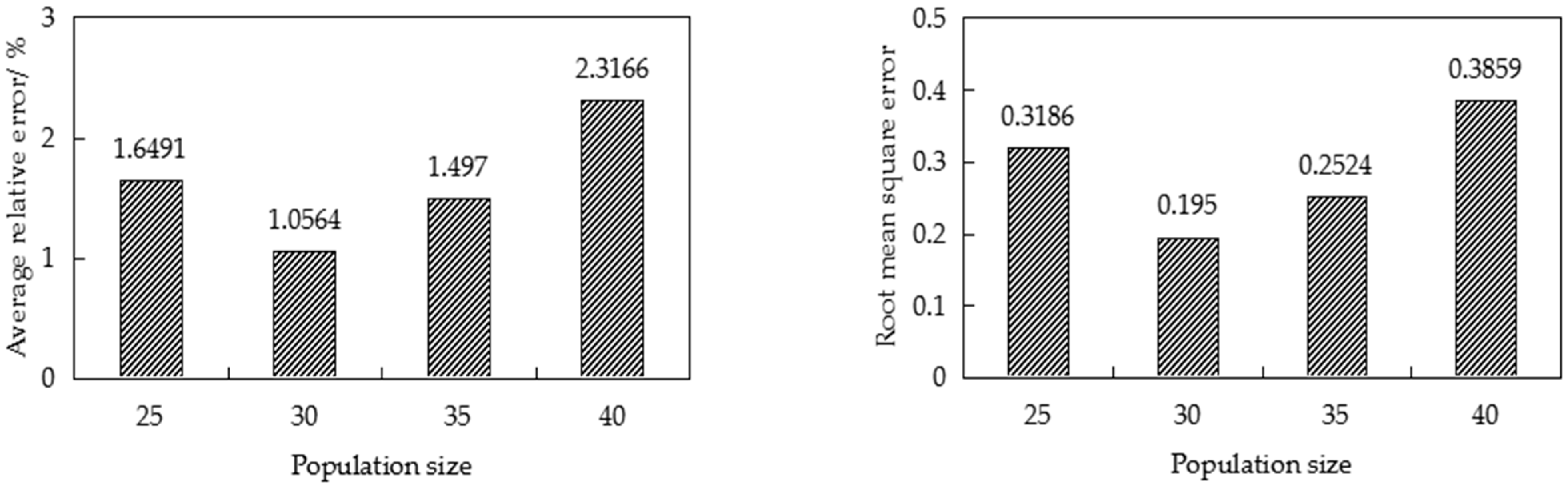
5.1. The Influence of Population Size on the Prediction Accuracy of the Improved Model

When the number of hidden layer nodes is 6 and the number of iterations is 60, the population size is set to 25, 30, 35, and 40, and the prediction results and relative errors of the improved Elman neural network model are obtained, as shown in Table 6. The average relative errors and root mean square errors of the prediction results for the improved model are further calculated, and the results are shown in Figure 2.

Table 6. The prediction results and relative errors of the improved model under different population sizes.

Population Size	Prediction Sample Number	Experimental Value/(μA·cm−2)	WOA-ENN Model
			Prediction Result/(μA·cm−2)	Relative Error/%
25	1	17.1100	16.5199	3.4489
	2	15.4700	15.7332	1.7014
	3	11.4479	11.4466	0.0114
	4	16.2800	16.0633	1.3311
	5	11.8285	11.6212	1.7525
30	1	17.1100	17.0228	0.5096
	2	15.4700	15.7353	1.7149
	3	11.4479	11.3519	0.8386
	4	16.2800	16.5995	1.9625
	5	11.8285	11.8588	0.2562
35	1	17.1100	16.7513	2.0964
	2	15.4700	15.6250	1.0019
	3	11.4479	11.3832	0.5652
	4	16.2800	16.2003	0.4896
	5	11.8285	12.2226	3.3318
40	1	17.1100	16.5100	3.5067
	2	15.4700	15.8057	2.1700
	3	11.4479	11.3915	0.4927
	4	16.2800	15.9861	1.8053
	5	11.8285	11.4017	3.6082

Figure 2. The average relative errors and root mean square errors of the prediction results under different population sizes.

From Table 6 and Figure 2, it can be seen that the maximum relative errors, the average relative errors, and the root mean square errors of the prediction results show a trend of first decreasing and then increasing with the increase in the population size. Therefore, a larger population size does not mean better prediction accuracy of the model. When the population size is 40, the average relative error (2.3166%) and the root mean square error (0.3859) of the prediction results are the largest. When the population size is 30, the average relative error (1.0564%) and the root mean square error (0.195) of the prediction results are the smallest. With the increase in the population size, the global search ability is enhanced, which improves the prediction accuracy of the improved model. When the population size exceeds a certain value, the running time of the algorithm increases, and it is easy to fall into the local optimal solution, which has a negative impact on the prediction performance. Therefore, a reasonable population size is helpful to improve the accuracy of the model. In addition, it can be seen that the prediction accuracy of the improved Elman neural network model under different population sizes is always higher than that of the traditional model when the number of hidden layer nodes is 6. Therefore, the whale optimization algorithm used in this paper is feasible to predict the corrosion rate of 3C steel.

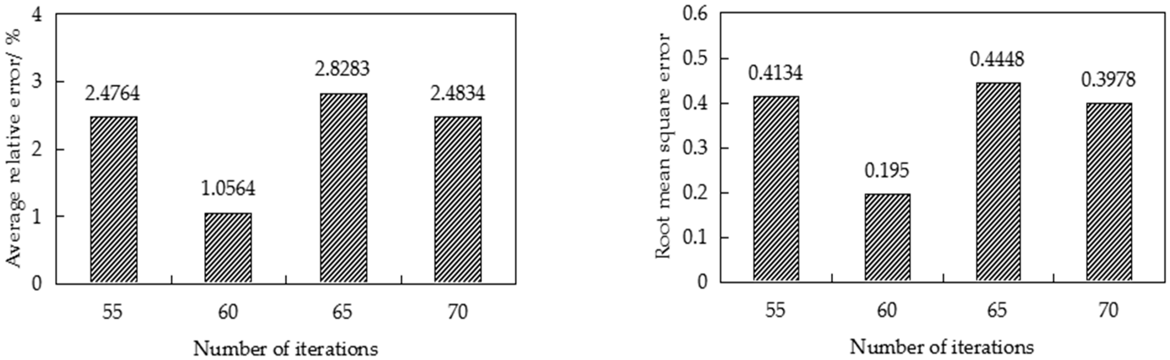
5.2. The Influence of the Number of Iterations on the Prediction Accuracy of the Improved Model

When the number of hidden layer nodes is 6 and the population size is 30, the number of iterations is set to 55, 60, 65, and 70, and the prediction results and relative errors of the improved Elman neural network model are obtained, as shown in Table 7. The average relative errors and root mean square errors of the prediction results for the improved model are further calculated, and the results are shown in Figure 3.

Table 7. The prediction results and relative errors of the improved model under different number of iterations.

Number of Iterations	Prediction Sample Number	Experimental Value/(μA·cm−2)	WOA-ENN Model
			Prediction Result/(μA·cm−2)	Relative Error/%
55	1	17.1100	17.4691	2.0988
	2	15.4700	15.7327	1.6981
	3	11.4479	11.4925	0.3896
	4	16.2800	16.5802	1.8440
	5	11.8285	11.0772	6.3516
60	1	17.1100	17.0228	0.5096
	2	15.4700	15.7353	1.7149
	3	11.4479	11.3519	0.8386
	4	16.2800	16.5995	1.9625
	5	11.8285	11.8588	0.2562
65	1	17.1100	16.4264	3.9953
	2	15.4700	15.9497	3.1008
	3	11.4479	11.8543	3.5500
	4	16.2800	16.5745	1.8090
	5	11.8285	11.6290	1.6866
70	1	17.1100	16.5504	3.2706
	2	15.4700	15.0315	2.8345
	3	11.4479	11.3506	0.8499
	4	16.2800	16.6330	2.1683
	5	11.8285	12.2181	3.2937

Figure 3. The average relative errors and root mean square errors of the prediction results under different number of iterations.

From Table 4 and Table 7, it can be seen that the maximum relative errors of prediction results for the improved model are lower than those of the traditional model. It can be seen from Figure 3 that the average relative errors and root mean square errors of the prediction results decrease first, then increase, and finally decrease with the increase in the number of iterations. Therefore, the larger the number of iterations does not mean that the prediction accuracy of the improved model is better.

When the number of iterations is small, there will be a problem of poor fitting effect, which results in low prediction accuracy. When the number of iterations exceeds a certain value, the overfitting phenomenon is prone to occur, which has a negative impact on the prediction accuracy of the network model and can also result in a waste of computing time and resources.

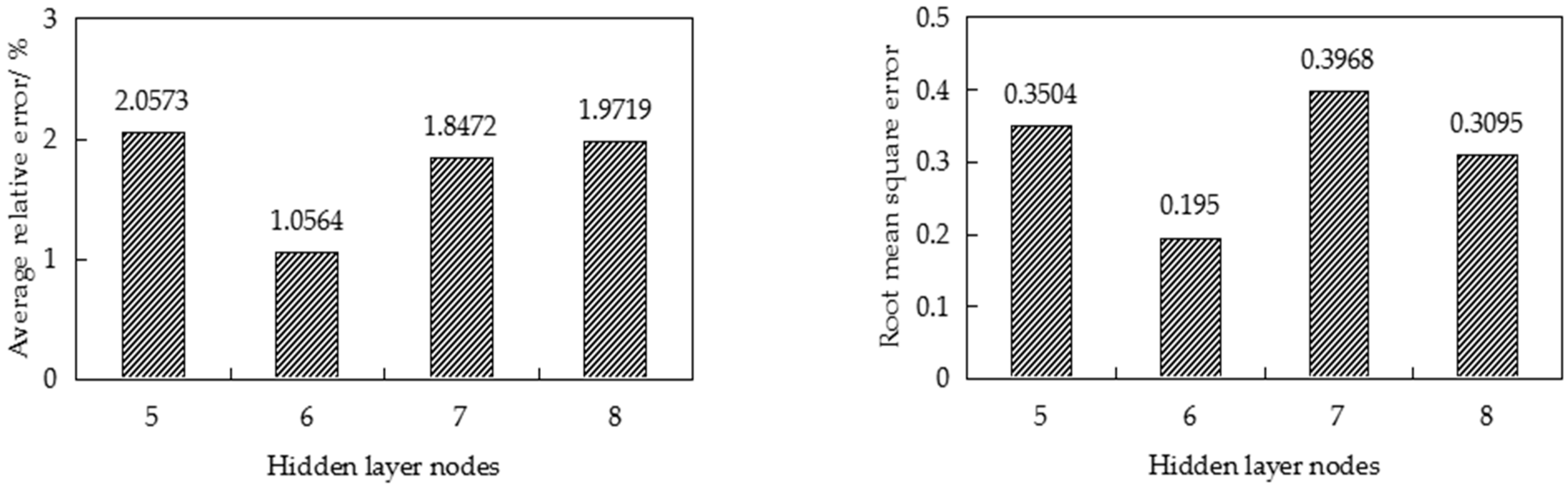
5.3. The Influence of the Number of Hidden Layer Nodes on the Prediction Accuracy of the Improved Model

When the number of iterations is 60 and the population size is 30, the number of hidden layer nodes is set to 5, 6, 7, and 8, and the prediction results and relative errors of the improved Elman neural network model are obtained, as shown in Table 8. The average relative errors and root mean square errors of the prediction results for the improved model are further calculated, and the results are shown in Figure 4.

Table 8. The prediction results and relative errors of the improved model under different hidden layer nodes.

Hidden Layer Nodes	Prediction Sample Number	Experimental Value/(μA·cm−2)	WOA-ENN Model
			Prediction Result/(μA·cm−2)	Relative Error/%
5	1	17.1100	16.5970	2.9982
	2	15.4700	15.8669	2.5656
	3	11.4479	11.4278	0.1756
	4	16.2800	16.4886	1.2813
	5	11.8285	11.4422	3.2658
6	1	17.1100	17.0228	0.5096
	2	15.4700	15.7353	1.7149
	3	11.4479	11.3519	0.8386
	4	16.2800	16.5995	1.9625
	5	11.8285	11.8588	0.2562
7	1	17.1100	16.3024	4.7200
	2	15.4700	15.6952	1.4557
	3	11.4479	11.4302	0.1546
	4	16.2800	16.0504	1.4103
	5	11.8285	11.6516	1.4955
8	1	17.1100	17.4694	2.1005
	2	15.4700	15.8684	2.5753
	3	11.4479	11.8365	3.3945
	4	16.2800	16.4643	1.1321
	5	11.8285	11.7508	0.6569

Figure 4. The average relative errors and root mean square errors of the prediction results under different hidden layer nodes.

It can be seen from Table 8 and Figure 4 that the maximum relative error, the average relative error, and the root mean square error of the prediction results are the lowest when the number of hidden layer nodes is 6. With the increase in the number of hidden layer nodes, the average relative errors of the predicted results decrease first and then increase. In addition, the root mean square errors show a trend of decreasing first, then increasing, and finally decreasing with the increase in the number of hidden layer nodes. When the number of hidden layer nodes is small, the network cannot learn and train well, so the prediction accuracy is poor. When the number of hidden layer nodes increases, the training samples are well fitted, so the prediction accuracy is better at this time. As the number of hidden layer nodes further increases, the complexity of the network increases, and overfitting is prone to occur. At this time, the prediction accuracy decreases (the average relative error increases).

6. Conclusions

• In view of the advantages of the whale optimization algorithm and the shortcomings of the Elman neural network, an improved Elman neural network model for corrosion rate prediction was established. The results showed that the average relative error and root mean square error of the improved model were significantly lower than those of the traditional model, so its prediction accuracy was higher than that of the traditional model.
• In the application process of the improved Elman neural network model, the population sizes, the number of iterations, and the number of hidden layer nodes have a great influence on the prediction results. With the increase in the number of hidden layer nodes and the population sizes, the average relative errors of the prediction results decrease first and then increase. With the increase in the number of iterations, the average relative errors of the prediction results decrease first, then increase, and finally decrease. Therefore, a larger number of hidden layer nodes, iterations, and population sizes does not mean higher prediction accuracy.
• The whale optimization algorithm can simulate the search process of whales and find the optimal solution, which has faster convergence speed and higher global search ability. In addition, the whale optimization algorithm can continuously optimize the initial weights and thresholds of the Elman neural network during the iteration process, which helps to improve the prediction accuracy of the Elman neural network. Although the whale optimization algorithm has many advantages in the application process, it still has some shortcomings. The prediction performance of the whale optimization algorithm will be affected by the parameter setting, and the relevant parameters need to be adjusted in the application process. In addition, the algorithm may lead to slower convergence speed when dealing with high-dimensional problems.

References

- Paul, S.; Mondal, R. Prediction and computation of corrosion rates of A36 mild steel in oilfield seawater. J. Mater. Eng. Perform. 2018, 27, 3174–3183. [Google Scholar] [CrossRef]
- Ferry, M.; Wan Nik, W.B.; Mohd Noor, C.W. The influence of seawater velocity to the corrosion rate and paint degradation at mild steel plate immersed in sea water. Appl. Mech. Mater. 2014, 554, 218–221. [Google Scholar] [CrossRef]
- Wang, X.W.; Ren, J.; Li, Z.L.; Li, Y.T. Research progress of vapor phase corrosion inhibitors in marine environment. Environ. Sci. Pollut. Res. 2022, 29, 88432–88439. [Google Scholar] [CrossRef] [PubMed]
- Zadeh Shirazi, A.; Mohammadi, Z. A hybrid intelligent model combining ANN and imperialist competitive algorithm for prediction of corrosion rate in 3C steel under seawater environment. Neural Comput. Appl. 2017, 28, 3455–3464. [Google Scholar] [CrossRef]
- Lee, S.; Narayana, P.L.; Seok, B.W.; Panigrahi, B.B.; Lim, S.G.; Reddy, N.S. Quantitative estimation of corrosion rate in 3C steels under seawater environment. J. Mater. Res. Technol. 2021, 11, 681–686. [Google Scholar] [CrossRef]
- Zou, Y.; Wang, J.; Zheng, Y.Y. Electrochemical techniques for determining corrosion rate of rusted steel in seawater. Corros. Sci. 2011, 53, 208–216. [Google Scholar] [CrossRef]
- Wang, J.; Meng, J.; Tang, X.; Zhang, W. Assessment of corrosion behavior of steel in deep ocean. J. Chin. Soc. Corros. Prot. 2007, 27, 1–7. [Google Scholar]
- Khadom, A.A. Comparison of mathematical and artificial neural network models for inhibition of fuel oil ash under high temperature corrosion. Corros. Eng. Sci. Technol. 2016, 51, 278–284. [Google Scholar] [CrossRef]
- Paul, S. Estimation of corrosion rate of mild steel in sea water and application of genetic algorithms to find minimum corrosion rate. Can. Metall. Q. 2010, 49, 99–106. [Google Scholar] [CrossRef]
- Kamrunnahar, M.; Urquidi-Macdonald, M. Prediction of corrosion behavior using neural network as a data mining tool. Corros. Sci. 2010, 52, 669–677. [Google Scholar] [CrossRef]
- Chen, X.Y.; Yuan, Z.M.; Zheng, Y.P.; Liu, W. Prediction of carbon steel corrosion rate based on an alternating conditional expectation (Ace) algorithm. Chem. Technol. Fuels Oils 2016, 51, 728–739. [Google Scholar] [CrossRef]
- Sattar, A.M.A.; Faruk, E.O.; Gharabaghi, B.; McBean, E.A.; Cao, J. Extreme learning machine model for water network management. Neural Comput. Appl. 2019, 31, 157–169. [Google Scholar] [CrossRef]
- Boukhari, Y.; Boucherit, M.N.; Zaabat, M.; Amzert, S.; Brahimi, K. Optimization of learning algorithms in the prediction of pitting corrosion. J. Eng. Sci. Technol. 2018, 13, 1153–1164. [Google Scholar]
- Poonguzhali, V.; Kannan, T.D.B.; Umar, M.; Sathiya, P. Application of ANN Modelling and GA Optimization for Improved Creep and Corrosion Properties of Spin-Arc Welded AA5083-H111 Alloy. Russ. J. Non-Ferrous Met. 2020, 61, 188–198. [Google Scholar] [CrossRef]
- Lee, K.E.; Aziz, I.B.A.; Jaafar, J.B. Adaptive multilayered particle swarm optimized neural network (AMPSONN) for pipeline corrosion prediction. Int. J. Adv. Comput. Sci. 2017, 8, 499–508. [Google Scholar]
- Liu, J.C.; Wang, H.T.; Yuan, Z.G. Forecast model for inner corrosion rate of oil pipeline based on PSO-SVM. Int. J. Simul. Process Model. 2012, 7, 74–80. [Google Scholar] [CrossRef]
- Wang, X.M.; Zhang, J.D.; Liu, Y.F.; Zhang, G. Modified ARIMA prediction model based on Elman neural network. J. Shanghai Marit. Univ. 2023, 44, 57–61. [Google Scholar]
- Liang, Y.F.; Xu, J.N.; Wu, M. Elman neural network based on particle swarm optimization for prediction of GPS rapid clock bias. J. Nav. Univ. Eng. 2022, 34, 41–47. [Google Scholar]
- Mirjalili, S.; Lewis, A. The Whale Optimization Algorithm. Adv. Eng. Softw. 2016, 95, 51–67. [Google Scholar] [CrossRef]
- Haghnegahdar, L.; Wang, Y. A whale optimization algorithm-trained artificial neural network for smart grid cyber intrusion detection. Neural Comput. Appl. 2020, 32, 9427–9441. [Google Scholar] [CrossRef]
- Wang, Z.B.; Zhao, L.H. Prediction of Loess Landslides Deformation Using Elman Neural Network Model Based on Genetic Algorithm and Particle Swarm Optimization. J. Geod. Geodyn. 2023, 43, 679–684. [Google Scholar]
- Yin, M.; Ke, P.; Zhang, C.R. An improved whale optimization algorithm with multiple strategies. J. Wuhan. Univ. Sci. Technol. 2023, 46, 145–152. [Google Scholar]
- Wu, L.; Mei, J.T.; Zhao, S. Pipeline damage identification based on an optimized back-propagation neural network improved by whale optimization algorithm. Appl. Intell. 2023, 53, 12937–12954. [Google Scholar] [CrossRef]
- Vaheddoost, B.; Guan, Y.Q.; Mohammadi, B. Application of hybrid ANN-whale optimization model in evaluation of the field capacity and the permanent wilting point of the soils. Environ. Sci. Pollut. Res. 2020, 27, 13131–13141. [Google Scholar] [CrossRef]
- Shang, Z.H.; He, Z.S.; Song, Y.R.; Yang, Y.; Li, L.; Chen, Y.H. A Novel Combined Model for Short-Term Electric Load Forecasting Based on Whale Optimization Algorithm. Neural Process. Lett. 2020, 52, 1207–1232. [Google Scholar] [CrossRef]
- Tang, C.J.; Sun, W.; Xue, M.; Zhang, X.; Tang, H.W.; Wu, W. A hybrid whale optimization algorithm with artificial bee colony. Soft Comput. 2022, 26, 2075–2097. [Google Scholar] [CrossRef]
- Kaur, G.; Gill, S.S.; Rattan, M. Whale Optimization Algorithm Approach for Performance Optimization of Novel Xmas Tree-Shaped FinFET. Silicon 2022, 14, 3371–3382. [Google Scholar] [CrossRef]
- Chakraborty, S.; Saha, A.K.; Sharma, S.; Chakraborty, R.; Debnath, S. A hybrid whale optimization algorithm for global optimization. J. Ambient. Intell. Humaniz. Comput. 2023, 14, 431–467. [Google Scholar] [CrossRef]
- Zhou, J.; Zhu, S.L.; Qiu, Y.G.; Armaghani, D.J.; Zhou, A.N.; Yong, W.X. Predicting tunnel squeezing using support vector machine optimized by whale optimization algorithm. Acta Geotech. 2022, 17, 1343–1366. [Google Scholar] [CrossRef]
- Jin, W.B.; Tian, Z.; Xiong, X.W.; Yang, Y.F.; Fan, C.Y. Prediction of 3C steel corrosion rate in the marine environment based on extreme learning machine. J. Saf. Environ. 2022, 22, 778–785. [Google Scholar]
- Chen, Z.; Liu, B.; Zhang, Y.; Yang, Y.B.; Tian, Y.Y. Prediction of wax deposition rate in pipeline by optimizing Elman neural network model with improved aquila optimizer. Sci. Technol. Eng. 2023, 23, 8179–8186. [Google Scholar]
Disclaimer/Publisher’s Note: The statements, opinions and data contained in all publications are solely those of the individual author(s) and contributor(s) and not of MDPI and/or the editor(s). MDPI and/or the editor(s) disclaim responsibility for any injury to people or property resulting from any ideas, methods, instructions or products referred to in the content. |
© 2024 by the authors. Licensee MDPI, Basel, Switzerland. This article is an open access article distributed under the terms and conditions of the Creative Commons Attribution (CC BY) license (https://creativecommons.org/licenses/by/4.0/).