Impact of Injection Rate on Flow Mixing during the Refining Stage in an Electric Arc Furnace

Abstract

During the refining stage of electric arc furnace (EAF) operation, molten steel is stirred to facilitate gas/steel/slag reactions and the removal of impurities, which determines the quality of the steel. The stirring process can be driven by the injection of oxygen, which is carried out by burners operating in lance mode. In this study, a computational fluid dynamics (CFD) platform is used to simulate the liquid steel flow dynamics in an industrial-scale scrap-based EAF. The CFD platform simulates the three-dimensional, transient, non-reacting flow of the liquid steel bath stirred by oxygen injection to analyze the mixing process. In particular, the CFD study simulates liquid steel flow in an industrial-scale EAF with three asymmetric coherent jets, which impacts the liquid steel mixing under different injection conditions. The liquid steel mixing is quantified by defining two variables: the mixing time and the standard deviation of the flow velocity. The results indicate that the mixing rate of the bath is determined by flow dynamics near the injection cavities and that the formation of very low-velocity regions or ‘dead zones’ at the center of the furnace and the balcony regions prevents flow mixing. This study includes a baseline case, where oxygen is injected at 1000 SCFM in all the burners. Two sets of cases are also included: The first set considers cases where oxygen is injected at a reduced and at an increased uniform flow rate, 750 and 1250 SCFM, respectively. The second set considers cases with non-uniform injection rates in each burner, which keep the same total flow rate of the baseline case, 3000 SCFM. Comparison between the two sets of simulations against the baseline case shows that by increasing the uniform flow rate from 1000 to 1250 SCFM, the mixing time is reduced by 10.9%. Moreover, all the non-uniform injection cases reduce the mixing time obtained in the baseline case. However, the reduction in mixing times in these cases is accompanied by an increase in the standard deviations of the flow field. Among the non-uniform injection cases, the largest reduction in mixing time compared to the baseline case is 10.2%, which is obtained when the largest flow rates are assigned to coherent jets located opposite each other across the furnace.

1. Introduction

An electric arc furnace (EAF) is a low-carbon emission steelmaking route widely adopted by the steel industry worldwide. Specifically, the EAF route can reduce the carbon emissions produced by the traditional blast furnace/basic oxygen furnace (BF-BOF) route by up to 63% [1]. Since the iron and steel industry produces ~6% of the global CO₂ emissions, and 71% of the iron and steel production utilizes the BF-BOF route [1,2], transition to EAF as the main route in the steelmaking industry is necessary in order to reach the carbon emission goals established for 2050. The flexibility of EAF operation, along with the control over steel temperature and grades it provides, enables the production of multiple steel products. The EAF primarily uses electrical energy with some chemical energy to melt and refine ferrous scrap and produce steel.

A typical EAF operation can be distinguished into four stages: charging, preheating, melting of scrap/iron substrates, and refining and tapping of liquid steel. In the preheating stage, the temperature of the ferrous charge is increased to facilitate its melting. In the melting stage, the ferrous charge is exposed to chemical reactions (due to oxidation reactions and burners) and electrical heating that melt the charge and produce a molten bath. In modern high-power EAFs, electrical heating accounts for 50–60% of the energy supplied. The refining stage refers to the period during which the molten bath is exposed to chemical–physical processes, such as supersonic oxygen injection into the steel, to refine and obtain (tapping) the desired liquid steel chemistry and temperature.

The refining stage reactions are controlled by the local concentration of species and flow properties of the liquid steel. These reactions can be enhanced by stirring forces as they increase the flow by mixing. For this reason, technologies such as O₂ injection through lances, bottom gas injection (BGI), and electromagnetic stirring (EMS) are applied in the refining stage [3]. The BGI technology is extensively applied in ladle furnaces. However, the application of BGI to EAF operation has challenges. These challenges are related to the height of the molten steel, which is variable in the EAF case, and the low ratio of liquid height to furnace diameter seen in EAF as compared to the ladle (3–5 times lower). As a result, large spouts may form at the bath surface in EAF, which affects the arc stability [3]. The EMS concept is an old one, but it has not been extensively commercialized in EAFs. Electric arcs in EAF generate electromagnetic forces, although these forces are weak. The installation of coils at the bottom of the EAF, where low-frequency current is applied, has demonstrated a significant stirring impact on the molten bath [4]. Recent implementations of EMS in EAF have shown significant improvements in thermal stratification, decarburization rates, and electrode consumption [5]. However, as mentioned earlier, EMS technology is not widely implemented. A well-established technology used in the refining stage of EAF is oxygen injection from lances. In this case, oxygen is injected into the molten steel through jets located above the liquid steel in order to stir it, remove impurities, and provide the right slag foaming. Once the injected oxygen dissolves in the liquid steel, the oxygen reacts with the carbon in the liquid to generate in-bath oxygen and CO bubbles, which generate turbulence and further stir the molten bath [6].

All these technologies aim to increase mixing in the molten bath to promote reactions during the refining stage. Although it is known that mixing is controlled by forces such as electromagnetics forces, buoyancy, momentum provided by flow injection (BGI or top oxygen injection), and CO bubble dynamics, the impact of specific forces on bath mixing is not well understood. Research on mixing efficiency in multiphase fluid flows has been conducted in numerous scenarios, such as channels and serpentine mixers [7,8,9,10], as well as in steelmaking processes. For instance, Li et al. [11] utilized the volume of fluid (VOF) multiphase model integrated with a discrete phase model (DPM) to describe the gas and liquid two-phase flow in a steelmaking converter that included top and bottom blowing. The study concluded that the buoyancy-driven bubbles are the driving force behind the majority of the evolved stirring energy in the converter. Interestingly, it was found that mixing efficiency was higher when three bottom tuyeres were used instead of two or four. This application is similar to the phenomenon produced in the refining stage in the EAF, where continuous blowing of oxygen into the liquid bath forms bubbles and induces stirring. Duan and Wei [12] analyzed the flow in an argon oxygen decarburization (AOD) converter with combined side–top blowing. The fluid mixing characteristics were investigated by studying the effect of rotation of the side-blowing gas jet and the influence of varying the blowing volume. The results indicate that improved mixing efficiency can be achieved by rotating the gas jet under the same blowing volume, which also improves the agitation.

Extensive flow analysis has been conducted in ladles, where water models have provided data needed for phenomena understanding and model validation. It is possible to translate this knowledge to the EAF operation, as similar flow features can be observed in both ladles and EAF (i.e., [13]). Zhu et al. [14] used an experimental water model and mathematical modeling to study mixing phenomena in a gas-stirred ladle. Similar to Li et al. [11], Zhu et al. [14] showed that the arrangement of tuyeres played a major role in the flow mixing. In particular, it was found that a single tuyere located at an off-centric position led to the shortest mixing time. The results also showed a significant impact of the angle of blowing on bath mixing and that mixing is enhanced by increased gas flow rate, although the latter had a secondary role. The study proposed a correlation to determine the mixing time in the ladle configuration. Amaro-Villeda et al. [15] also analyzed the flow mixing in ladles and added the effect of slag properties into the analysis. The results showed that slag thickness has a negative impact on mixing, as it leads to higher energy dissipation. Also, it was found that the range of energy dissipated to the top layer of the ladle is 4–12%. The authors concluded that due to the multiple injection parameters, such as gas flow rate, number of nozzles, and position of nozzles, it is difficult to establish an optimal number of injectors for flow mixing. Cheng et al. [16] investigated the mixing process in a ladle that was scaled down to 1:3 from a 150 t industrial ladle. This configuration considered both side and bottom blowing. In this study, velocity fields and diffusion paths obtained by computational fluid dynamics (CFD) simulations were compared with experimental data, showing good agreement. The results also showed that mixing time depends on agitation power and the associated uniformity of the flow velocity. Overall, it was concluded that shorter mixing times were obtained with a side-blowing configuration compared with bottom blowing.

Chen et al. [6] developed a CFD platform to compute the refining process in industrial-scale EAFs. The model computed the coherent jets and liquid baths separately, avoiding the restrictions set by the supersonic flow on the computational time needed during the refining simulations. The models were then integrated back to compute the in-bath decarburization process. The results obtained with this methodology showed that bubble stirring is a major mechanism for promoting flow homogenization in the molten steel bath. Also, a significant impact of oxidation reactions on the liquid temperature was identified. Decarburization reactions were observed mostly around the cavities produced by the penetrating jets. Li [17] analyzed the mixing process in an electric arc furnace with bottom stirring. This study considered both computational and experimental methods to analyze a 1:7 model of a 30-ton EAF. The impact of parameters such as diameter and location of plugs on flow mixing was analyzed. The results showed that off-center blowing of gas into the liquid bath improved the intensity of stirring and the mixing rate. Moreover, the mixing rate did not show a significant increase with plug diameter, but increasing the number of plugs had a positive impact on the flow homogenization.

The research mentioned above quantifies the metrics for mixing and homogenization in a liquid bath, but it also demonstrates that the mixing characteristics are somehow specific to the particular scenario. In order to determine the conditions for optimal flow mixing in EAF, it is necessary to model the EAF with the conditions and geometry to be used in the actual operation. This study aims to determine the flow features and the conditions for optimal mixing in an industrial-scale EAF, where oxygen is injected through coherent jets. Since the flow rate can be varied in the co-jets within a certain range, this study analyzes the impact of having different flow rates in the co-jets during EAF operation. Different scenarios are computed to understand how the injection rates modify the flow field and, as a result, the mixing process. A CFD platform introduced by Chen et al. [6] is used to perform the calculations. This investigation focuses on the flow field developed in the steel bath as a result of the oxygen injection, and thus the reactions occurring during the refining stage are not considered (‘cold flow’ approach). The simulations do consider the combustion reactions of the shrouded flame in the coherent jets.

2. Methodology

2.1. Description of the Integrated CFD Platform for EAF Refining Simulations

This section contains a brief description of the computational model used to simulate the oxygen injection in liquid bath scenarios. For more information, including details of the model validation and CFD implementation, the reader is referred to [6].

The model uses three steps to set up the physical boundaries of the domain and perform the computations. These steps are defined according to three physical processes occurring concurrently during the EAF refining: (1) oxygen blowing into the liquid bath via co-jet burners, (2) the interaction between the coherent jet and the liquid steel, and (3) the stirring of the bath due to high-intensity jet injection. This methodology ensures the simulation accuracy of the refining stage without compromising the computation resources, as the supersonic regime is restricted to the first step only. These three steps are summarized as follows:

• The supersonic coherent jet is simulated first based on the injection conditions of the burners operating in lance mode. This simulation assumes a steady-state condition, as the impact of the liquid bath on co-jet operation is expected to be minor. This step provides velocity profiles and composition of the injecting flow from the tip of the burner to the surface of the bath.
• Outputs from the coherent jet simulation are used to estimate the cavities formed by the jets on the surface of the liquid bath.
• The computational domain for the refining simulation is created based on the actual geometry of the industrial-scale EAF and the geometry of cavities calculated in step 2. This domain includes the liquid bath only. A transient simulation is performed in the computational domain where oxygen is injected at the cavities, at the rate provided by the coherent jet simulation solution.

The refining CFD platform used in step 3 is able to compute multiple species and reactions. However, in this study, the refining reactions are not computed, and it is assumed that only one liquid species is present in the liquid bath (steel). Next, each of the steps listed above is further described.

2.2. Simulation of the Supersonic Coherent Jet Burners (Steady State Simulation)

The supersonic coherent jet simulation considers an open space under furnace conditions. The coherent jet injection is solved as a compressible, non-isothermal, steady-state flow. The solver used is a compressible solver implemented in ANSYS Fluent version 2019. The continuity equation solved for the coherent jet is as follows:

$$\nabla .\left(\rho \overrightarrow{v}\right)=0$$

(1)

The momentum equation is constructed as follows:

$$\nabla .\left(\rho \overrightarrow{v}\overrightarrow{v}\right)=-\nabla p+\nabla .\left(\stackrel{̿}{\tau }\right)+\rho \overrightarrow{g}+\overrightarrow{F}$$

(2)

where $\rho$, $\overrightarrow{v}$, $p$, $\stackrel{̿}{\tau }$, $g$, and $\overrightarrow{F}$ are the density, velocity vector, static pressure, stress tensor, gravity acceleration, and the external body force, respectively. Moreover, the energy conservation equation can be written as follows:

$$\nabla .\left[\overrightarrow{v}(\rho E+p)\right]=\nabla .\left[\left(k+\frac{c_p.{\mu }_t}{{Pr}_t}\right)\nabla \mathrm{T}-\sum _j{h}_j\overrightarrow{J_J}+({\stackrel{̿}{\tau }}_{eff}.\overrightarrow{v})\right]+S_h,$$

(3)

Here, $E$, $k$, $c_p$, and ${\mu }_t$ are the total energy that corresponds to the sensible enthalpy $h$, thermal conductivity, specific heat, and turbulent viscosity, respectively. ${Pr}_t$ is the turbulent Prandtl number (equal to 0.85) for the $k-\epsilon$ turbulence model, $\overrightarrow{J_J}$ is the diffusion flux of substance $j$. $S_h$ is the volumetric heat source, which includes the heat of chemical reactions. Note that even though the simulations do not include refining reactions, step 1 accounts for combustion reactions of the shrouded flame present in the co-jets. The turbulence viscosity is modeled as:

$${\mu }_t=C_{\mu }\rho \frac{k^2}{\epsilon },$$

(4)

where the constant is modified in order to include the influence of entrained ambient gas [18] as follows:

$$C_{\mu }=\frac{0.09}{C_T}.$$

(5)

The modification of the turbulent viscosity is loaded into the CFD software via a user-defined function (UDF) code. Figure 1 shows the interaction of the coherent jet with the liquid bath. This interaction will generate a cavity in the surface of the liquid steel, which is computed in the second step of the CFD setup.

2.3. Calculation of the Cavity Produced by the Coherent Jet in the Liquid Bath

For the second step, a cavity is estimated on the surface of the liquid bath based on the impingement of the supersonic jet on the bath [19]. The jet momentum transfer and oxygen delivery are calculated in this step to estimate the cavity shape and size. Based on the energy balance calculation, the momentum transferred by the jet flow to the liquid steel is given by:

$$P_{s,avg}=\alpha {\rho }_{O_2}{v_{O_2}}^{2}A=\frac{\alpha {\rho }_{O_2}A}{{\rho }_s}{\left[\frac{1}{∆z}{\int }_{z2}^{z1}{v}_{O_2}\left(z\right)dz]\right]}^2$$

(6)

The amount of deliverable oxygen from the jet to the liquid bath is expressed as:

$$m_{O_{2,avg}}=\frac{1}{∆z}{\int }_{z2}^{z1}{m}_{O_2}\left(z\right)dz$$

(7)

The cavity is used to inject oxygen into the liquid bath and induce in-bath stirring. About 6% of the momentum is transferred from the jet to the bath due to the dampening effects of the slag layer and viscosity effects [6]. The jet cavity design is integrated into the refining simulation, with the cavity being part of the boundaries of the EAF domain (to be shown in Section 2.3). The main characteristics needed from the coherent jet simulation are the velocity of the jet reaching the bath and the amount of oxygen reaching the bath. The shape of the cavity is assumed to be a 3D paraboloid which follows the mathematical expression

$$z=\frac{(x^2+y^2)}{c},$$

(8)

where c is the constant needed to be defined by a given volume and depth of the cavity. The volume of the cavity [20] can be obtained by

$$V=\frac{\pi {\rho }_j{v_j}^2{d_j}^2}{4g{\rho }_s},$$

(9)

where ${\rho }_j$ and ${\rho }_s$ are the primary densities of the jet and liquid steel, and $v_j$ and $d_j$ are the jet velocity and jet diameter of the nozzle, respectively. The jet penetration depth is an empirical formula derived by Ishikawa et al. [21], which mathematically describes the indentation created by the coherent jet in the liquid bath. This is expressed as

$$D={\gamma }_{h_0}{e}^{-\frac{{\sigma }_{1}L}{{\gamma }_{h_0}cos\theta }}$$

(10)

$${\gamma }_{h_0}={\sigma }_2\left(\frac{\dot{V}}{nd\sqrt{3}}\right)$$

(11)

Here, L is the distance between the nozzle exit and bath, ${\sigma }_1$ and ${\sigma }_2$ are constants equal to 1.77 and 1.67, respectively, derived from an experiment analysis [22], $\theta$ is the angle of the jet inclination and $n$ is the number of nozzles (1 in this study). The size and shape of the cavity vary according to the velocity of the jet reaching the bath, the diameter of the burner nozzle, and the density of the liquid bath.

2.4. Stirring of the Bath Due to Jet Injection (Transient Simulation)

Finally, the third part of the CFD platform is the simulation of the region containing the liquid steel bath generated in the furnace after all the scrap melts. The simulation incorporates the solution of the Navier–Stokes equations into a finite volume scheme by using the ANSYS Fluent platform. Specifically, the computational solution is based on a Eulerian multi-phase, incompressible approach, where the primary phase is the molten liquid, and the secondary phase is the injected oxygen. The simulation uses the standard k-e model with standard wall functions. The boundary conditions for oxygen injection are provided by the coherent jet solution, and these are included in the refining simulation with a user-defined function. Figure 2 shows the computational domain considered during the refining simulations on the right side of the figure. This domain includes the cavities produced by the coherent jets.

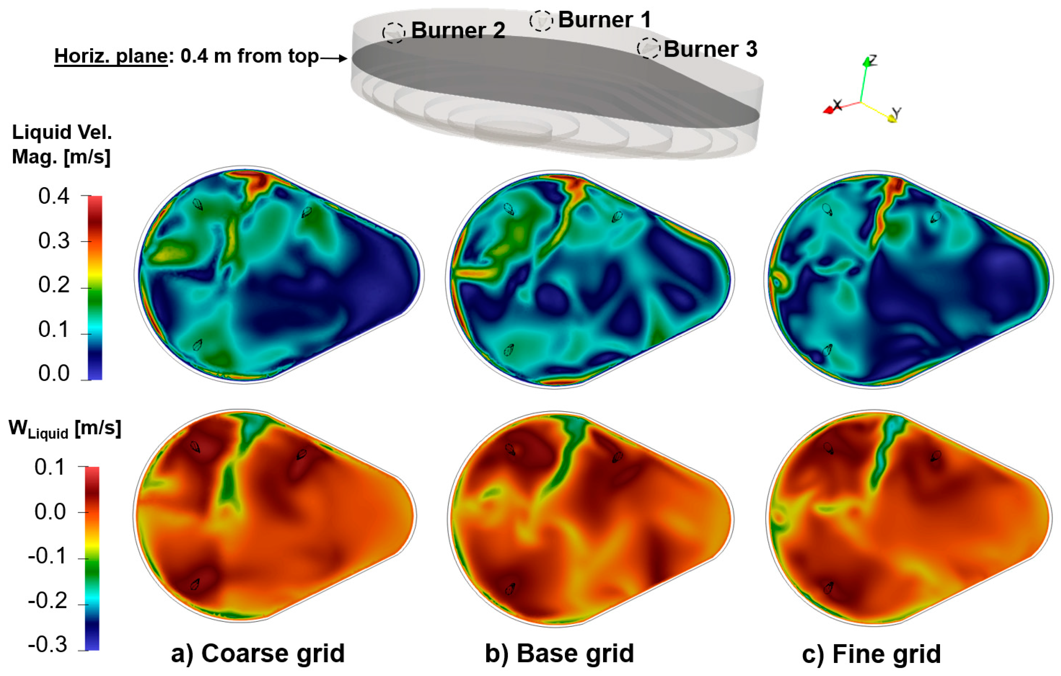
2.5. Grid Sensitivity Study

A grid resolution study was performed on the computational setup shown in Figure 2. Namely, a case with the same operation conditions was repeated by using a coarse (0.3 million cells), a base (0.6 million cells), and a fine grid (1.3 million cells). The results obtained at a plane located 0.4 m from the top (close to the oxygen injection burners) are shown in Figure 3. The top set of contours shows the liquid velocity magnitude, whereas the lower ones show the velocity in the vertical direction. All three grids show similar flow structures. In particular, regions with large velocity magnitudes are observed between burners 1 and 3, and a reduced velocity flow develops near the balcony. Moreover, the three grids develop similar flow fields of the vertical velocity component (W_Liquid), which show the impact of the jets on the vertical acceleration.

The main velocity components are listed in

Table 1. Results obtained with the three grid resolutions.

Grid	Number of Cells (Million)	Volume Averaged at Plane Located 0.4 m from the Surface (m3)			CPU Hours
		Uliquid	Vliquid	Wliquid
Coarse	0.3	−0.012	−0.020	0.0038	6464
Base	0.6	−0.009	−0.014	0.0027	6528
Fine	1.3	−0.006	−0.018	0.0022	7936

for the three grid resolutions. Overall, we see that the order of the magnitude of the flow velocities is the same, with flow values mostly approaching the results of the fine grid. The results in Figure 3 and Table 1 indicate that the results are not further modified by grid refining: both the qualitative and quantitative CFD predictions do not change significantly when the grid is further refined, and the base grid is able to capture the flow features observed in the fine grid, where the number of cells is duplicated. The cases to be presented and discussed in this study were completed by using the base grid resolution.

2.6. Operation Conditions of Case Simulations

The simulations for this research use conditions of an actual EAF operation provided by EVRAZ North America. The EAF operation includes three co-jets working in lance mode. The shrouding gas in the co-jets is natural gas, which is injected into rings located around the central nozzle, where oxygen is injected. The gases are injected at room temperature. In the simulations of the liquid bath interacting with the injected oxygen, the gas corresponds to oxygen and the liquid to molten steel. The parameter values used in this study are listed in

Table 2. Parameters used in the simulations.

Name	Variables	Value
Jet cavities	Quantity	3
Oxygen injection	Flow rates	750, 1000, 1250 SCFM (0.47, 0.63, 0.78 kg/s)
	Mass fraction of oxygen	100%
Liquid Steel	Density	7500 kg/m3
	Static temperature	1815 K (1542 C)
Coherent jet burner	Angle of inclination	45 degrees

. The simulations include two main sets of results. The first set assumes the same injection rate in all three jets of the EAF. This includes the baseline case, where oxygen is injected at 1000 SCFM (standard cubic feet per minute), a case with reduced injection rates (750 SCFM), and a third case with increased injection rates (1250 SCFM). The second set of cases includes variable injection rates in the three jets, where the 750, 1000, and 1250 SCFM rates are assumed at each jet, in different order. The specific conditions of the variable injection rate cases will be discussed in Section 3.3.

3. Results

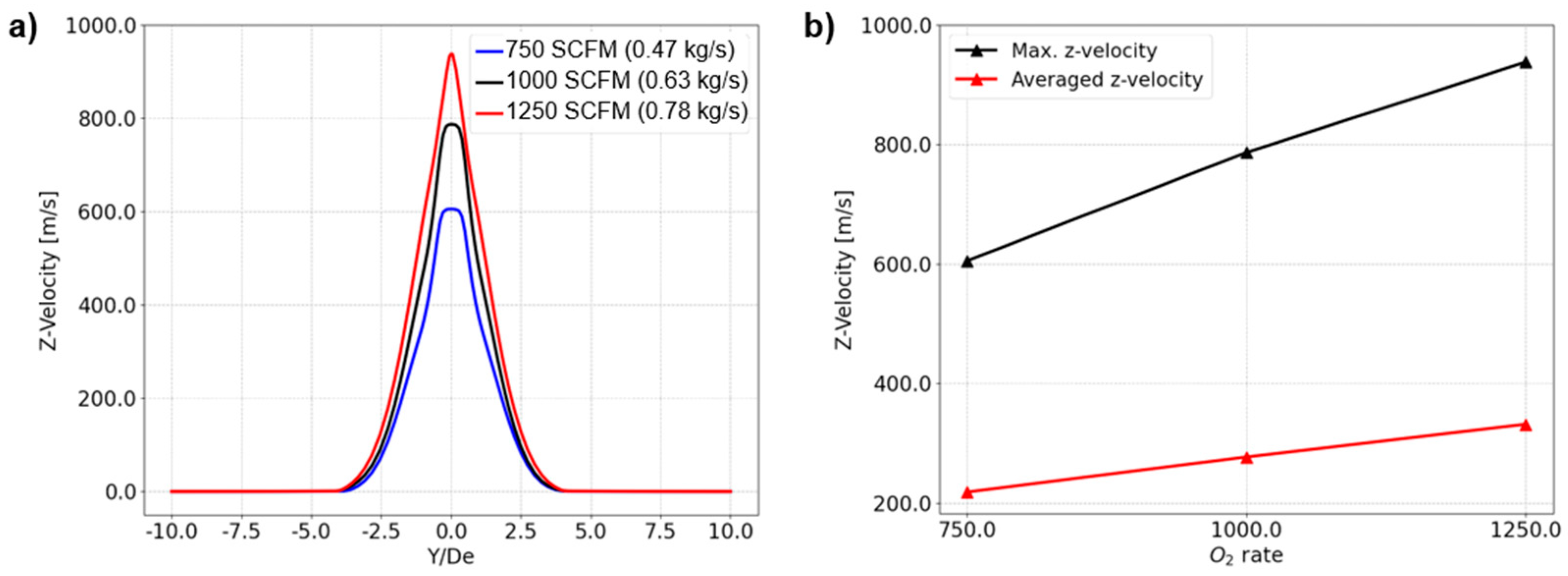
3.1. Impact of Flow Rate on the Coherent Jets’ Penetration Depth

The coherent jet CFD model is used to obtain the flow velocity and oxygen mass fraction of the gas injected by the burners (operating in lance mode) when it reaches the molten bath. As explained in Section 2.1, the flow features produced by the injected gas are used to compute the cavities that jets produce in the bath, which are part of the computational domain used in the refining simulations. Figure 4 shows the velocity magnitude contours generated by the three injection rates considered in this study: 750, 1000, and 1250 SCFM. The dashed line shows the location at which the flow profile is obtained. The flow profile information at this location is then used in the calculation of the bath cavities by using the procedure explained in Section 2.3. The distance from the left boundary to the dashed line (L = X/De = 30, where De is the diameter of the jet) corresponds to the distance from the tip of the burner to the surface of the molten bath.

The results in Figure 4 show an increase in velocity magnitude as the flow rate increases, as expected. In all cases, the larger flow velocities are observed along the jet centerline. It is observed that the flow velocity is maintained until around X/De = 50 for all cases. This implies that flow entrainment generated as the jet interacts with the environment does not prevent the jets from transferring momentum to the liquid bath. Figure 5a compares the velocity profile at X/De = 30 for the three injection rates. Increasing the flow rate from 1000 to 1250 SCFM leads to a 16% increase in the maximum velocity, whereas reducing the flow rate from 1000 to 750 SCFM reduces the maximum velocity by 30%. Figure 5b shows the maximum and averaged axial velocities (z-component) for the three flow rates considered in this study. The average velocities approach a linear behavior, as they increase by 21.3 and 19.4% when increasing the O₂ rate from 750 to 1000 SCFM and from 1000 to 1250 SCFM, respectively.

The results obtained by the coherent jet CFD model, shown in Figure 4 and Figure 5, are used to compute the cavities formed in the liquid bath. Figure 6 shows the cavities produced by the 750, 1000, and 1250 SCFM injection rates, and the variations in the volume and depth of the cavities with respect to the baseline case (1000 SCFM).

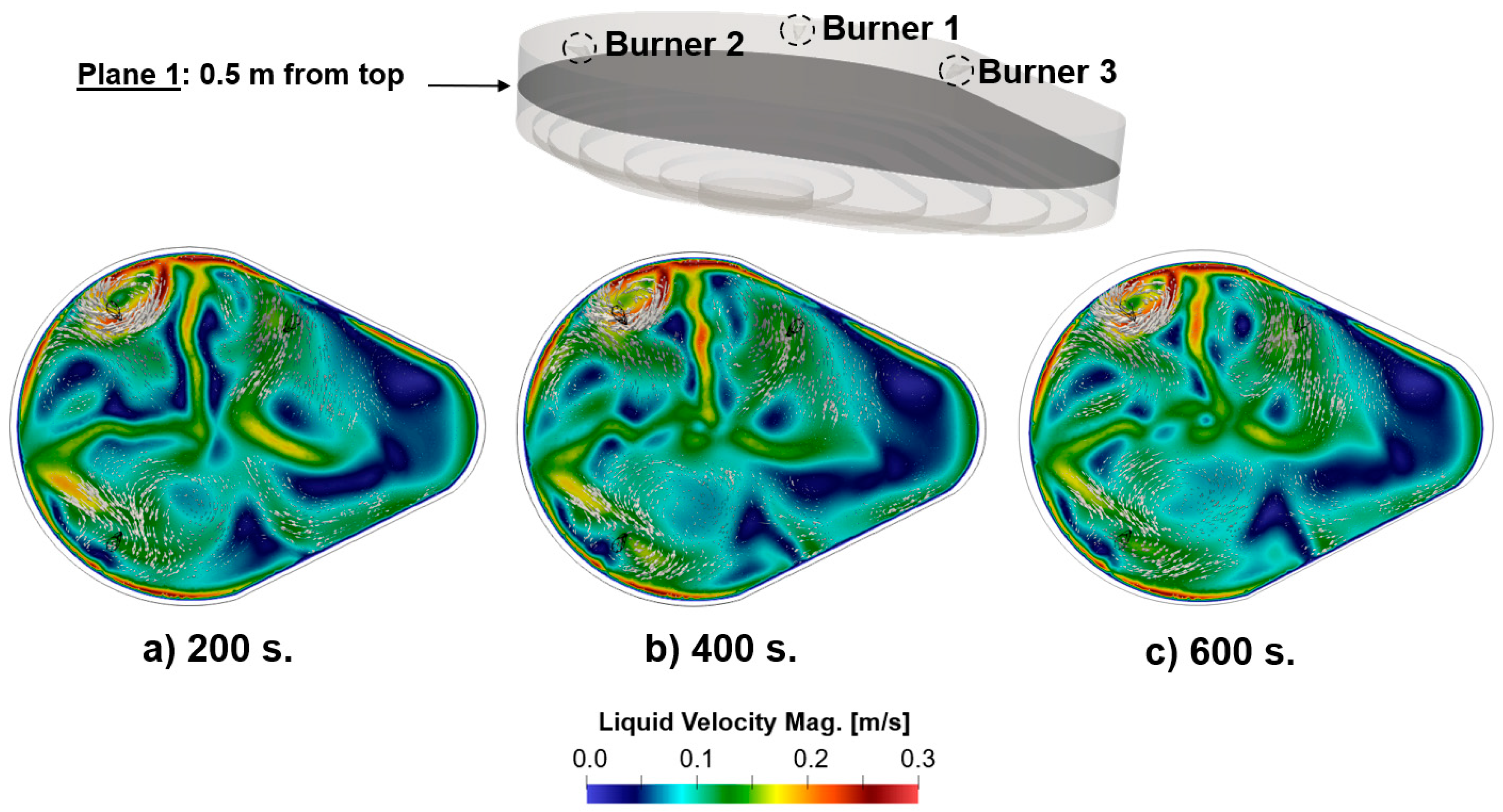
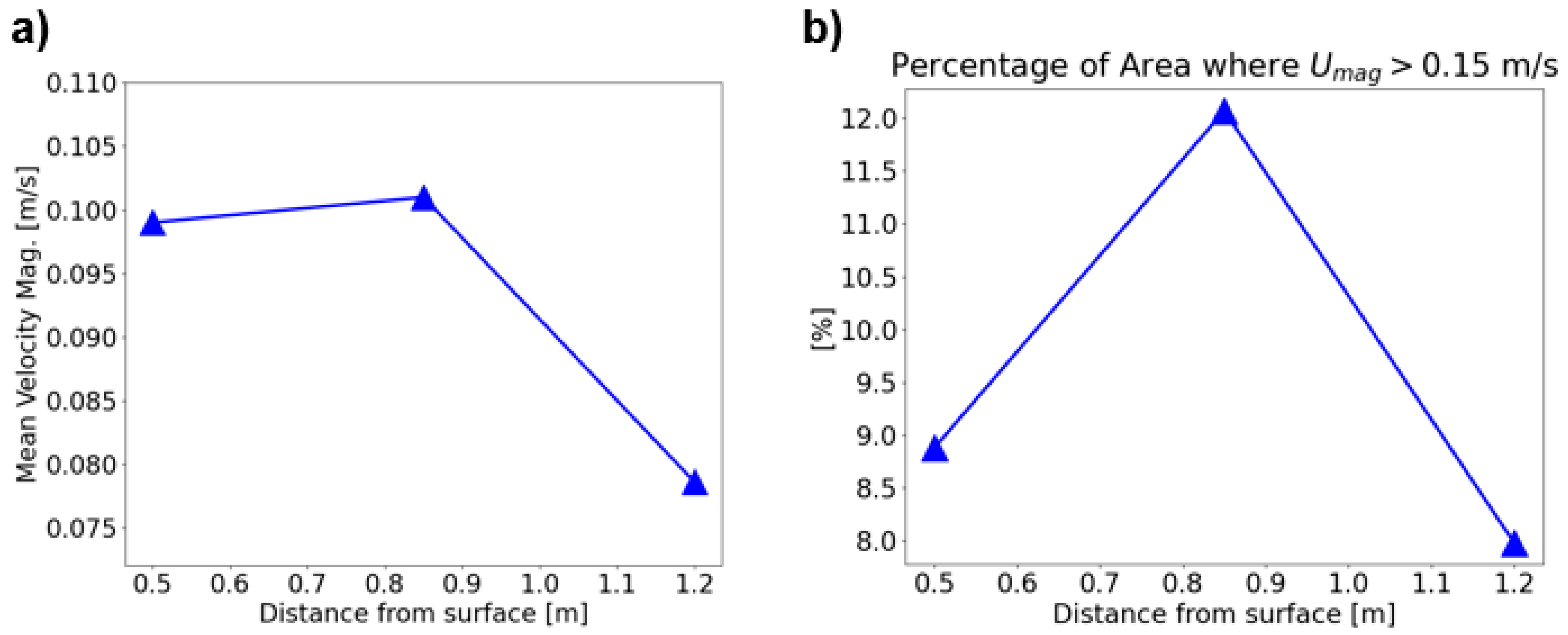
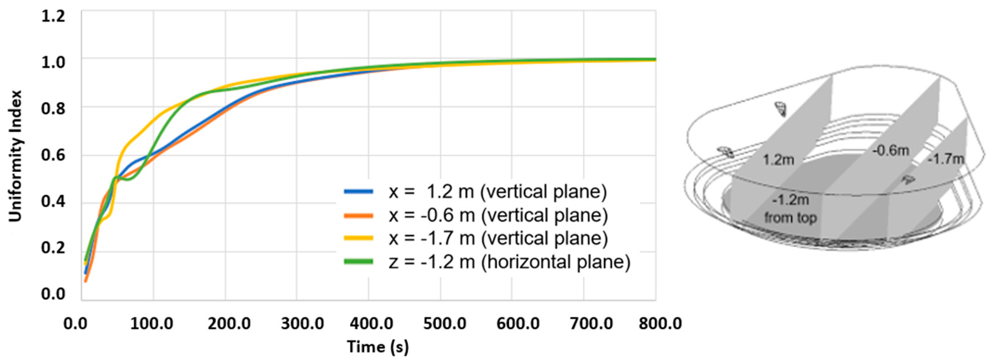
3.2. Baseline Results in the Steel Bath Domain

The baseline case considers oxygen injection at a rate of 1000 SCFM in all the burners, which operate in lance mode. Figure 7 shows the location of the burners in Figure 7a and the flow patterns associated with such injection rates after 600 s in Figure 7b. The flow pattern shows large fluid velocities near the burners, dropping significantly as the flow changes direction due to interactions with the walls and the flow injected from adjacent burners. Overall, the flow velocity magnitude decreases from around 5 m/s to 0.01–0.5 m/s. Moreover, considering the entire domain, the average velocity is 0.024 m/s in the horizontal direction and 0.068 m/s in the vertical direction. These average velocities agree with those reported in Ref [3]. The flow pattern is particularly non-uniform. The main reasons for the non-uniformity of the flow are the geometry of the furnace, the asymmetric distribution of the injectors, and the angle at which the oxygen is injected.

Figure 8 shows the instantaneous velocity magnitude on a plane located 0.5 m from the top of the domain. The velocity contours are computed at t = 200 s, 400 s, and 600 s. The contours also include the velocity vectors of the flow field. Figure 8a through 8c show that the flow field does not change significantly along these time intervals. At all times, the flow velocities are larger near burner 1, as a result of the interaction of burners 1 and 3. By contrast, the flow injection near burner 2 decays quickly as this is the only injection point on the lower side of plane 1. Flow recirculation is shown at burner 1, and adjacent to burners 2 and 3. Also, the flow velocity near the balcony of the furnace (right end of plane 1) approaches zero, which can be attributed to the ‘dead zone’ in the liquid steel flow domain. Low-velocity regions or ‘dead zones’ are also formed on the lower wall of the plane (in the region opposite burner 3), near the center of the domain, and near burner 2. The percentages of the dead-zone volumes (defined as those regions where V_mag < 0.05 m/s) are 6.3, 6.4, and 7.3% of the molten bath volume for time instants 200, 400, and 600 s, respectively. Overall, the flow features are consistent along the three time instances of the burner operation shown in Figure 8.

Figure 9 shows the instantaneous velocity magnitude and flow vectors of the liquid steel on three planes, at t = 600 s. The locations of the planes are shown at the top of the figure. The results show that flow intensity is larger near the top planes of the domain (planes 1 and 2) where the momentum is transferred by the jets. The main features observed in plane 1 (Figure 9a) are also seen in plane 2 (Figure 9b). Namely, large velocities develop near burner 1 and on the upper side of planes 1 and 2, towards the left end. Plane 2 is further inside the furnace (Figure 9b) and, overall, it shows similar flow intensity as compared to plane 1. The flow velocities are reduced in plane 3, taken 1.2 m from the surface of the liquid bath. In plane 3, the velocity magnitude does not exceed 0.2–0.25 m/s, although recirculation patterns similar to those observed in planes 1 and 2 are maintained.

Figure 10 shows the mean velocity magnitude and the region of high-intensity flow in the planes indicated in Figure 9. Figure 10a shows that the mean velocity magnitude remains similar in the upper regions of the liquid bath, with a slight increase in the flow intensity when going from 0.5 to 0.85 m into the bath. Figure 10a also shows that the mean velocity magnitude decays by 28% on a plane located 1.2 m below the bath surface. This location is 0.15 m from the bottom of the furnace. Figure 10b, in turn, shows the percentage of the areas of planes 1–3 where the velocity magnitude is above 0.15 m/s. Here, it is shown that the region with significant flow intensity occupies ~12% of plane 2, and less than 8% of plane 3.

Figure 11 extends the analysis by considering two vertical planes, which are shown at the top of the figure. Figure 11a shows plane 4, which is oriented towards the balcony of the furnace. Plane 4 shows larger liquid velocities on the left side, near the locations of burners 1 and 2. The flow vectors on the left side of plane 4 show a vertical recirculation produced by the interaction of the flow injected at burners 1 and 2 with the bottom of the furnace. Therefore, the asymmetric distribution of the burners at the top of the liquid bath leads to the formation of recirculation structures in the horizontal and vertical directions near burners 1 and 2, as shown in planes 1–3 (Figure 9) and plane 4 (Figure 11a). Figure 11b shows larger flow velocities on plane 5 than on plane 4 due to the vicinity of burners 1 and 3, although the recirculation pattern in this plane is weaker than in plane 4. Planes 4 and 5 show large velocity gradients through the domain due to the asymmetric distribution of the burners and geometry of the EAF. Figure 12 confirms these observations by indicating increases in the mean velocity and size of the region with higher flow intensity in plane 5 with respect to plane 4 of 15 and 183%, respectively.

The results in Figure 11 also suggest that the flow velocities and associated flow mixing would be increased by adding a fourth jet to the system. Namely, planes 4 and 5 show weak flows due to the presence of only one co-jet in the balcony. Since the balcony region is large, the stirring in the vertical direction is reduced away from burner 3, which is located near the wall of the balcony. Moreover, the balcony region extends the asymmetry of the bath horizontally, and the angle of injection of burner 3 (and burner 4 if it is included) could be modified so that the oxygen is injected towards the center of the balcony instead of the center of the liquid bath.

Figure 13 shows the instantaneous velocity components U_liquid, V_liquid, and W_liquid of the liquid steel on planes 1, 2, and 3 discussed earlier. The axis orientation is included at the bottom left of the figure. Figure 13a,b show that the flow intensity is larger on the left side of the planes, near burners 1 and 2. Figure 13b shows that U_liquid and V_liquid increase as the flow interacts with the end wall at the balcony. The W_liquid contours in Figure 13a show the flow structures produced vertically as a result of the oxygen injection. Namely, the oxygen injection produces the stirring of the liquid bath upwards. The W_liquid contours in Figure 13a also show negative velocities associated with the stirring, which determine the recirculating patterns seen in planes 4 and 5 in Figure 11. The overall intensity of flow vertical penetration decreases as we move into the liquid bath, and a much reduced W_liquid contour is observed at the furnace bottom in Figure 13c.

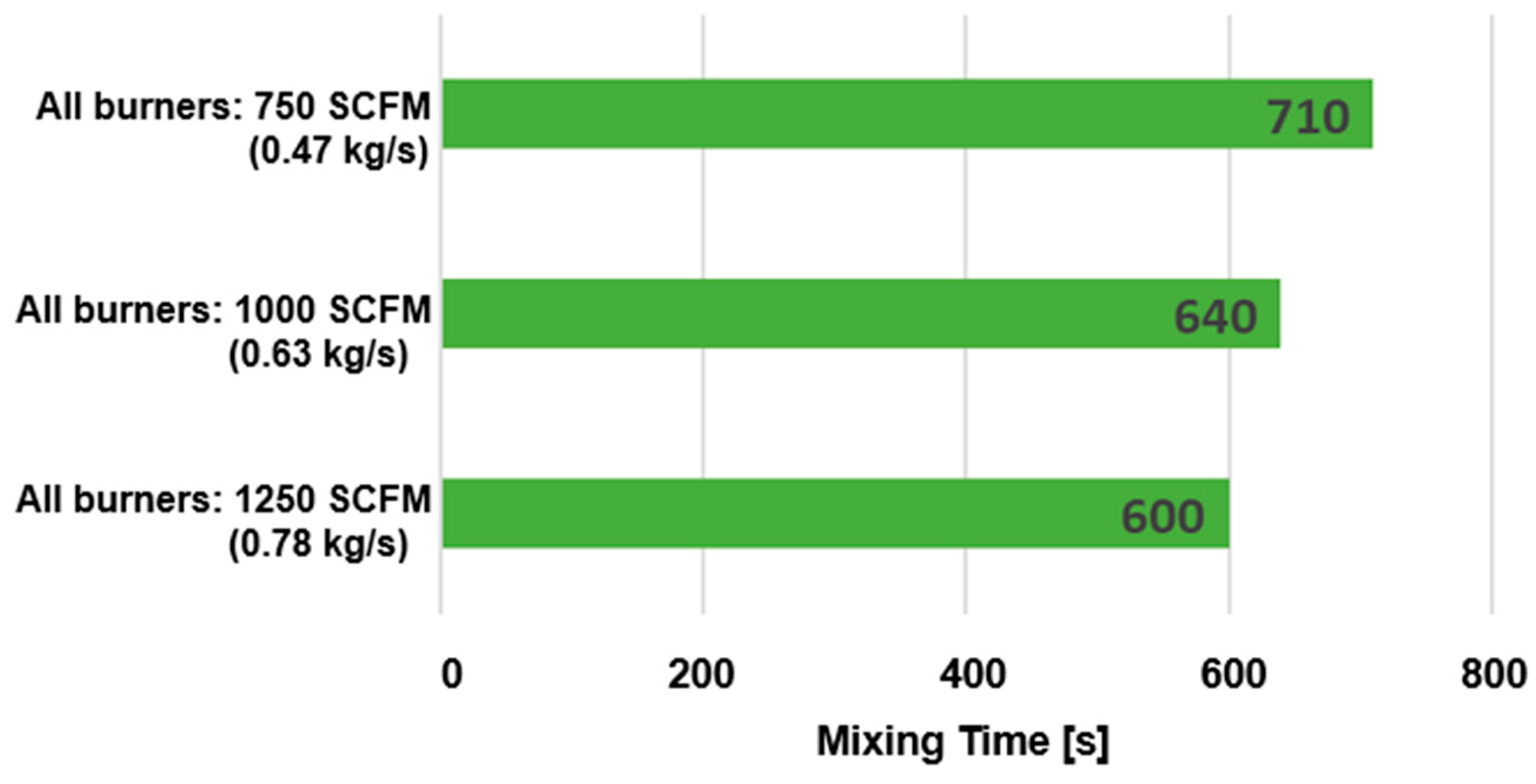
3.3. Effect of Total Flow Rate

The effect of both increasing and decreasing the flow rate of the burners is explored in this section. Specifically, two additional cases are simulated where the flow rates at the burners are uniformly increased by 25% and decreased by 25%. These are listed in

Table 3. Case conditions of the parametric study.

Cases	Coherent Jet Flow Rates (SCFM) (kg/s)				Stirring Energy (W/ton)
	Burner 1	Burner 2	Burner 3	Total Injection
1	1000 (0.63)	1000 (0.63)	1000 (0.63)	3000 (1.88)	0.078
2	1250 (0.78)	1250 (0.78)	1250 (0.78)	3750 (2.34)	0.104
3	750 (0.47)	750 (0.47)	750 (0.47)	2250 (1.41)	0.130

as cases 2 and 3, respectively. It should be noted that coherent jet burners are designed to operate at 20–30% of their factory-set flow rate, as this helps maintain the stability of the flame, and preserves maximum oxygen delivery to the bath.

Table 3 includes the stirring energy for cases 1–3. The stirring energy is computed based on the relation reported by Mazumdar and Guthrie [13], ε = g.Q/πR², where g is gravity acceleration, Q is the gas flow rate in Nm³/s, and R is the averaged radius of the furnace. Since the EAF geometry is asymmetric in this study, R is defined as the semi-sum of long and short lengths of the liquid surface, leading to R = 6.28 m.

The effect of increasing and decreasing the flow rate in the burners is shown in Figure 14, where these scenarios, in addition to the baseline case, are compared at t = 600 s. Figure 14b shows that the increased flow rate intensifies the flow near the burners, and leads to the formation of a ‘dead zone’ at the center of the furnace, where the flow velocity is negligible. The flow vectors in Figure 14b show a significant increase in the liquid velocity near burners 2 and 3, and near the walls, as compared to the baseline case. Figure 14c shows the case with a decreased flow rate. Here, the flow velocities are reduced throughout the domain, and the dead zone regions are the largest among the three scenarios.

In addition to the impact of the modified injection rates on the velocity magnitudes, changes in the injection rates also modify the flow patterns, reflected in the location of the recirculation zones and the formation of the dead zones. Figure 15 compares the three cases listed in Table 3 by computing the velocity magnitude on a plane taken along the centerline of the furnace, as shown at the top of the figure. Figure 15b shows that the increased flow rate case moves the recirculation region towards the left side of the plane, and makes the ‘jet’ type flow in the center of the domain (along the vertical direction) stronger than in the baseline case. The increased flow rate case strengthens the two vortices on the left side of the jet-type vertical flow. By contrast, when the flow rate is reduced in all the burners from 1000 to 750 SCFM, one vortex is observed near the left wall of the plane, and the flow penetration towards the bottom of the furnace weakens significantly (Figure 15c).

Figure 16 shows regions in the furnace domain where the instantaneous velocity magnitude is larger than 0.15 m/s for the baseline case and for the cases with increased and reduced flow injection rates. These regions confirm the highly asymmetric distribution of the flow velocities, as the larger velocities are obtained in the half of the domain that contains burners 1 and 2. Figure 16b shows that by increasing the flow injection from 1000 to 1250 SCFM, the regions containing velocities above 0.15 m/s extend towards the balcony of the furnace.

Figure 17 helps to illustrate the impact of increasing and reducing the injection rate uniformly in all the burners. Figure 17a shows that the mean velocity magnitude increases by 10% when increasing the flow rate from 750 to 1000 SCFM, and by 23% when increasing the flow rate from 1000 to 1250 SCFM. However, the impact on the size of the region where the flow velocity is significant (i.e., larger than 0.15 m/s) seems rather exponential, as it increases by 25% when increasing the flow rate from 750 to 1000 SCFM, and 210% when increasing the flow rate up to 1250 SCFM. Therefore, increasing the flow rate has a larger impact on extending the region where the jets stir the bath rather than increasing the liquid steel velocity itself.

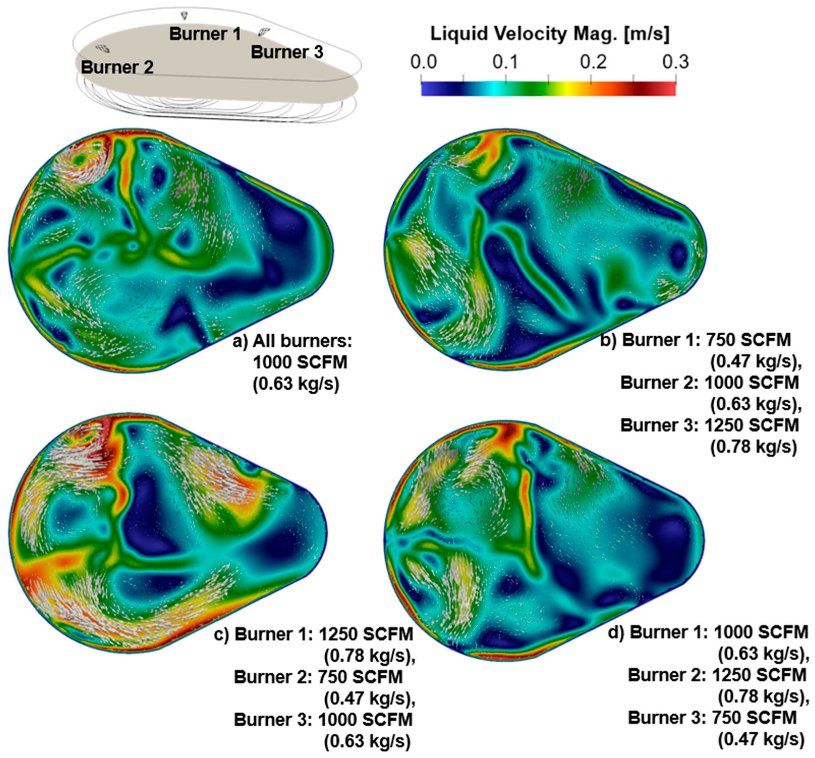
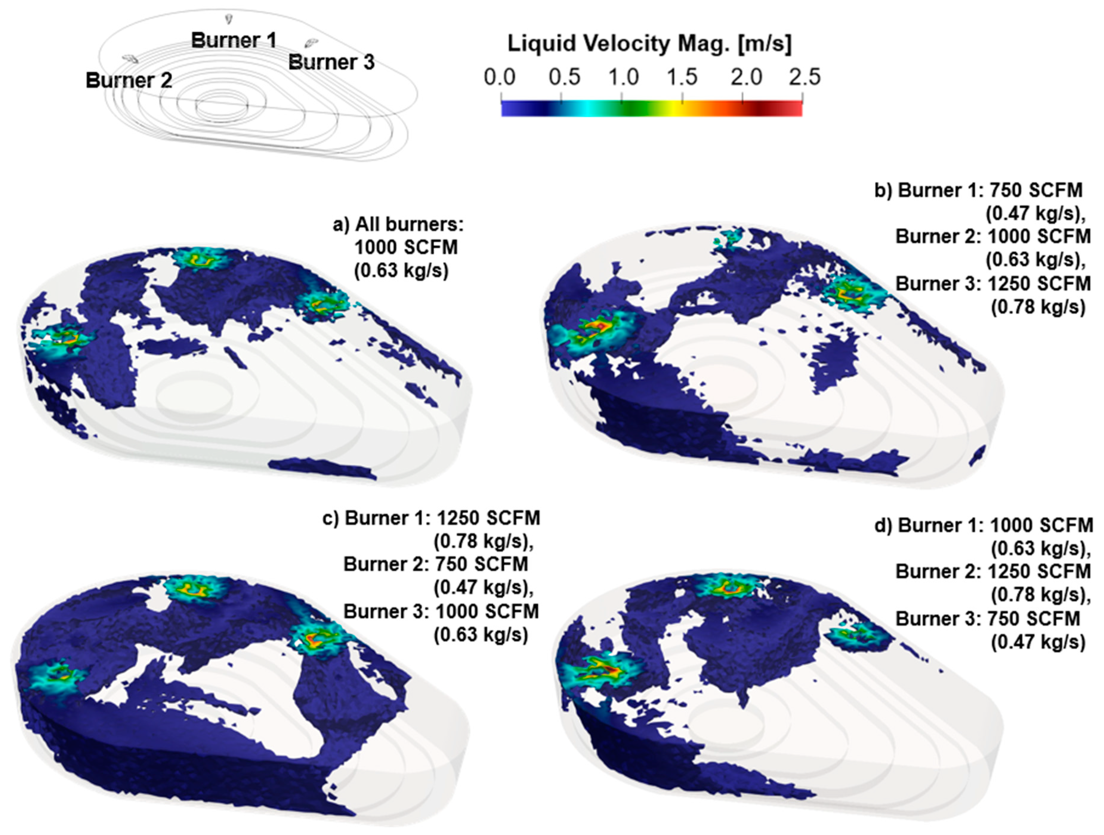
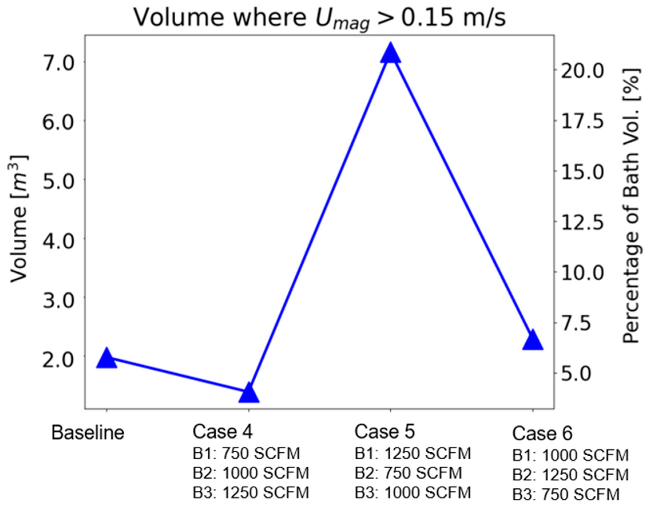
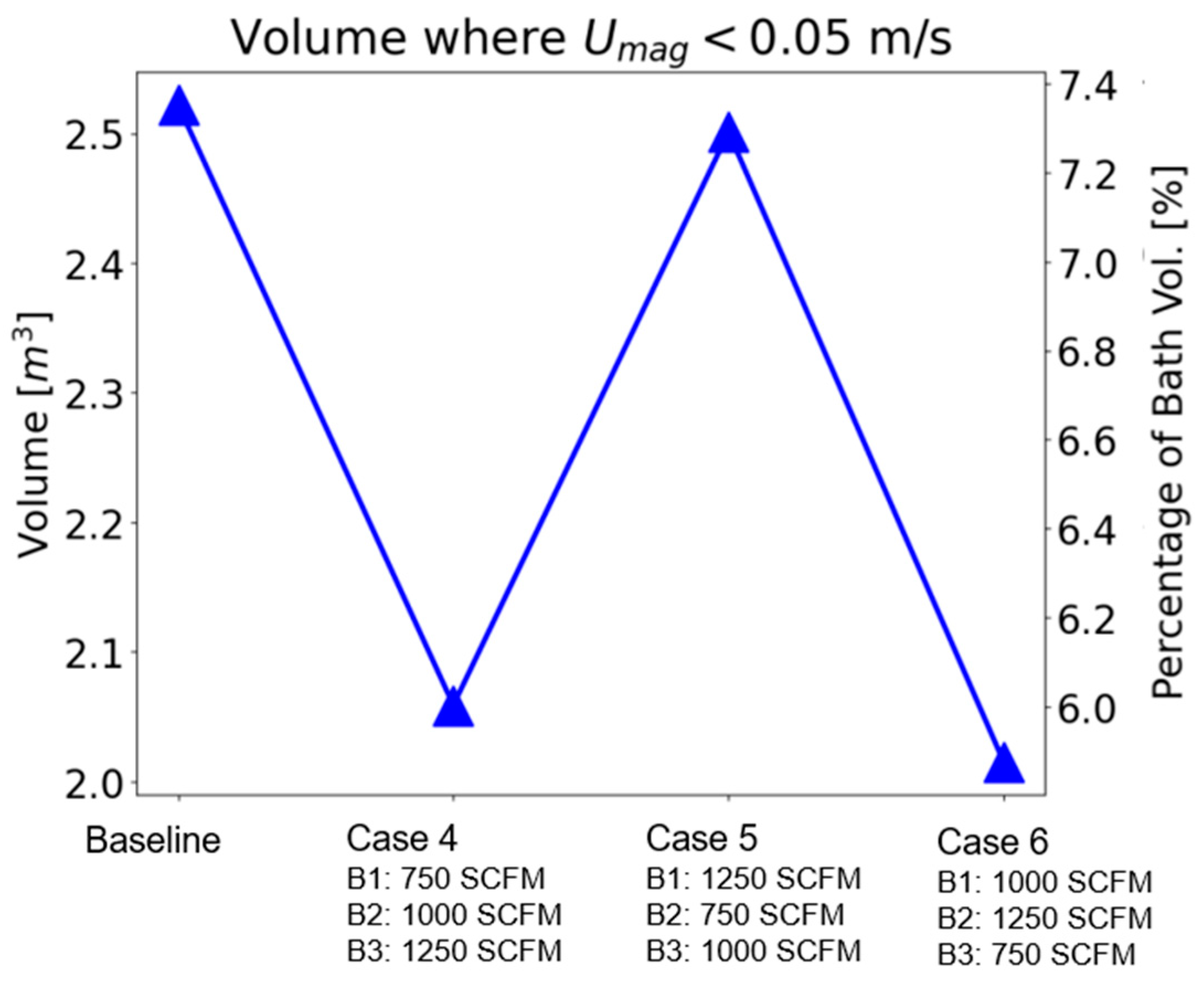
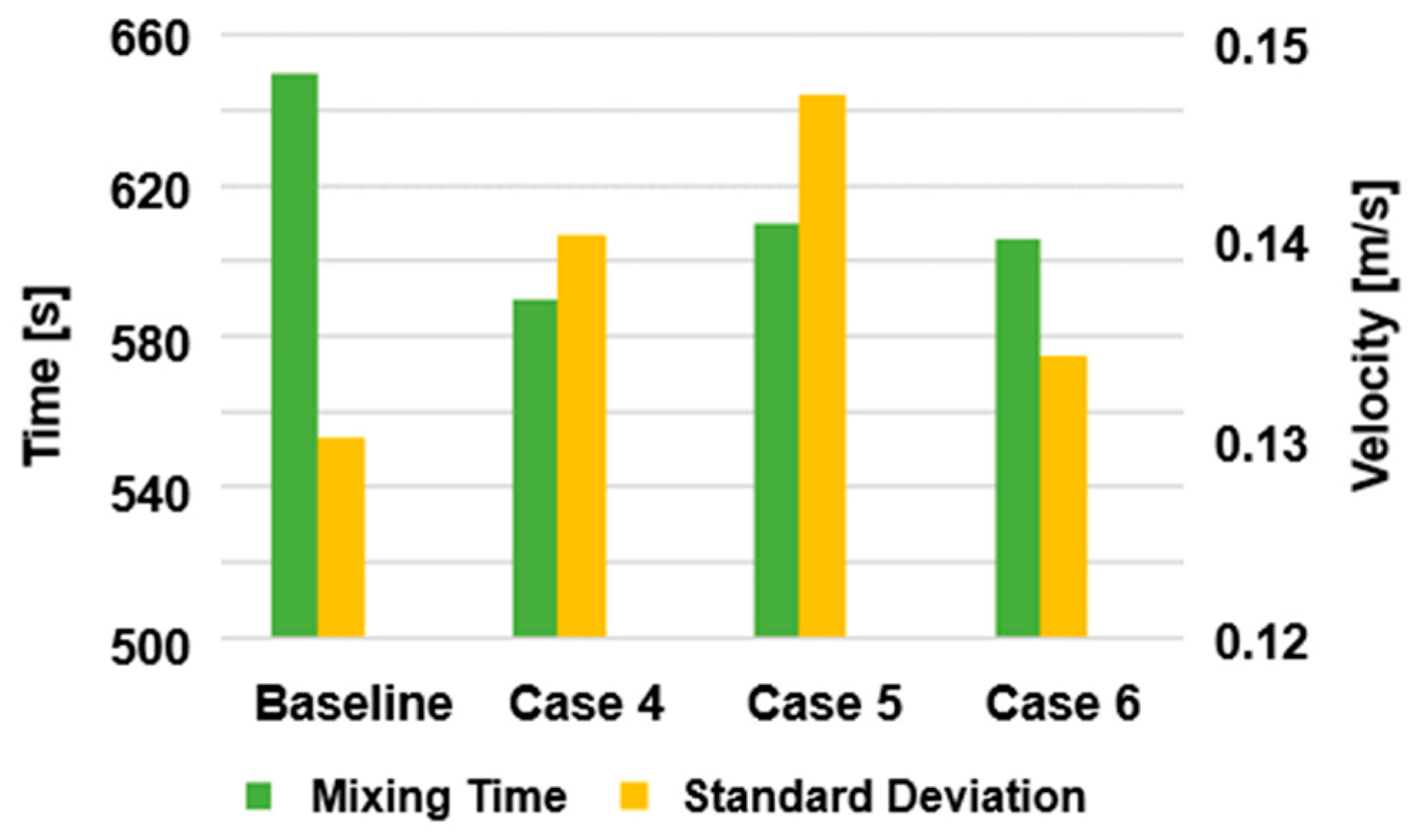
3.4. Effect of Non-Uniform Burner Flow Rates

The analysis performed in Section 3.2 and Section 3.3 is extended here to include individual variations in the flow rate of the coherent jets. This leads to non-uniform injection rate scenarios. Three cases are considered in this study, which are designated as cases 4 through 6 in

Table 4. Conditions of cases where the jet rates are varied individually.

Cases	Coherent Jet Flow Rates (SCFM) (kg/s)
	Burner 1	Burner 2	Burner 3	Total Injection
4	750 (0.47)	1000 (0.63)	1250 (0.78)	3000 (1.88)
5	1250 (0.78)	750 (0.47)	1000 (0.63)	3000 (1.88)
6	1000 (0.63)	1250 (0.78)	750 (0.47)	3000 (1.88)

.

The contours of the liquid velocities and flow vectors of the non-uniform injection scenarios at t = 600 s are shown in Figure 18. In these cases, the flow rate injected by the three burners combined is the same, 3000 SCFM, which differs from cases 1–3 where the total injection rate changed. In cases 4–6, the flow pattern varies significantly depending on the location of the burner that is increased or decreased with respect to the baseline rate of 1000 SCFM. Figure 18b shows the case where the largest flow rates are at burners 2 and 3. In this case, the dead zone region is increased in the center of the furnace as compared to the baseline due to the stirring driven mainly by burners that are located opposite each other. By increasing the flow rate in burner 1 and reducing it in burner 2 (Figure 18c) the largest flow rates are injected near the top side of the plane, where burners 1 and 3 are located. This also increases the flow velocities near burner 2, even though the flow rate in this burner is reduced to 750 SCFM. In this case, the flow velocities are larger than in the baseline case, although a dead zone region is formed in the center of the domain in addition to the one formed at the balcony. Finally, by setting burners 1 and 2 to the largest flow rates while reducing the injection rate at burner 3 (Figure 18d), the flow velocities are intensified as well, but the increase in the flow velocities is mostly on the left side of the plane view, whereas the right side and balcony region are exposed to low liquid velocities.

Figure 19 compares the flow velocities of liquid steel on a plane taken along the furnace centerline, towards the balcony region. In all four cases, there is a ‘jet’-type flow from the liquid surface toward the bottom of the furnace near the center of the plane. The location of this jet flow changes with the flow rate of the burners. In Figure 19a,d, the jet flow is seen closer to the center of the plane than in Figure 19b,c. In all cases, flow recirculation is observed to the left of the jet flow. The location and intensity of the jet flow are expected to have a significant impact on the mixing process, which will be analyzed in the next section.

Figure 20 shows the regions where the liquid flow velocities are larger than 0.15 m/s for the cases listed in Table 4. As mentioned earlier, the total flow rate is the same for all the cases, but clearly the stirring intensity is not, as the injection rate in each of the burners is modified. The largest flow intensity is seen in Figure 20c, and a moderated intensification of the flow is seen in Figure 20d. In these two cases, the burners injecting the largest flow rates, 1000 and 1250 SCFM, are located next to each other. By contrast, in Figure 20b the largest flow rates are applied by burners opposite each other (burners 2 and 3), and no significant difference with respect to the baseline case is observed.

Figure 21 shows the volume of the regions where the velocity magnitude is larger than 0.15 m/s for the baseline case and cases 4 through 6. These results show that the flow rate distribution in case 4 reduces the region of larger flow intensity obtained in the baseline case. Case 5 increases the large velocity region by 260% with respect to the baseline, whereas Case 6 increases the large velocity region by 15%.

The last set of results presented in this section corresponds to the W_liquid velocity computed at 0.5 m from the top of the liquid bath, for all six cases presented in this study (Figure 22). The W_liquid velocity is the velocity component that is perpendicular to the surface of the liquid bath, and it is expected to have a large impact on the reactions produced in the steel–slag interface and on the slag mixing during the actual operation of the EAF. Figure 22 shows three regions in each of the cases where W_liquid is positive (flow moving towards the bath surface). These regions correlate with the locations of the burners. Interestingly, the case with the reduced flow injection (750 SCFM, Figure 22a) shows larger W_liquid velocities than the baseline case and the case with increased flow injection (Figure 22b,c, respectively). These larger W_liquid velocities are observed near the walls, adjacent to the burners. However, Figure 22a also exhibits the larger regions with negligible W_liquid velocity among the three uniform injection cases.

Figure 22d–f show the cases with non-uniform injection rates. Among these results, Figure 22d shows the case with the smallest region containing zero or near zero W_liquid velocities. However, the largest W_liquid velocities are seen in Figure 22e. As mentioned earlier, the W_liquid velocity component is expected to impact the reactions near the steel/slag interface. In this paper, however, neither the reactions nor the presence of slag are considered, and the study is focused on the flow features resulting under different injection rates and the way this impacts the mixing rate. In the next section, the flow velocity variations and corresponding mixing rates are studied in more detail for the different injection scenarios shown in cases 1–6.

Figure 23 and Figure 24 complement the previous set of results by showing the regions where low velocities are produced. These results correspond to regions where the velocity magnitude is less than 0.05 m/s. The dead zones impact the mixing rate of the liquid bath as these regions are expected to take longer to stir, which will lead to the formation of velocity (and concentration) gradients in the bath. Figure 23 shows dead zones mainly in the central region and on the balcony of the furnace, for all the cases. The dead zones on the balcony are reduced in Figure 23b,c, as the flow rate of burner 3 located near this region is significant. The dead zones in the center of the domain are reduced in Figure 23d, as a result of the large flow rates imposed by burners 1 and 2, located nearby.

Figure 24 shows the size of the bath regions shown in Figure 23. It is shown that the non-uniform injection rates of the burners reduce the ‘dead zones’ size with respect to the baseline case. This reduction is minimal for case 5, but ~20% for cases 4 and 6. As mentioned earlier, the reduction in the size of the dead zones should have a positive impact on the efficiency of the mixing rate, which will be analyzed in the next section.

4. Discussion

In order to quantify the effect of injection rates on bath mixing, two parameters are defined: the mixing time, which is the time needed by any species to blend into the generated flow, and the standard deviation of the fluid flow velocity, which determines the homogeneity of the velocity field in the liquid bath.

The mixing time is computed by introducing a passive tracer in the generated flow, with a mass fraction $Y_{tracer}=1.0$. The uniformity index, which represents how a specified field variable varies over the domain, is used to calculate the mixing time. Specifically, the uniformity index is calculated as follows:

$$y_a=\frac{1}{V}\sum _{i=1}^n{\varnothing }_i\left|V_i\right|$$

(12)

where $\overline{{\varnothing }_i}$ is the local value of the field variable. In this study, $\overline{{\varnothing }_i}$ is given by $Y_{tracer}$. According to this definition, a uniformity index of 1 indicates a uniform concentration of the passive tracer throughout the domain.

The variation in the uniformity index with time can be calculated locally on selected planes along the simulation. This requires computing the uniformity index on a per area basis rather than per volume as given by Equation (12). Figure 25 shows the uniformity variation with the time of selected planes for the baseline case (1000 SCFM in all the burners). The planes where the uniformity index is computed are shown on the right side of the figure. The results in Figure 25 show how the uniformity index varies in time with the selected location, and how the uniformity index value eventually converges to ~1 at a similar time for all planes, around 640 s. In the results to be discussed next, the mixing time in each of the cases is determined by the time when the uniformity index calculated on a per volume basis (by using Equation (12)) reaches 0.95.

Figure 26 shows the mixing time for cases 1 (baseline, 1000 SCFM in all burners), 2 (1250 SCFM in all burners), and 3 (750 SCFM in all burners). This illustrates the effect of increasing and reducing the flow rate of the coherent jet on the mixing process. Namely, a 25% increase in the flow rate leads to a reduction of 6.7% in the mixing time, whereas by reducing the uniform flow rate by 25%, the mixing time increases by 10.9%.

Figure 27 compares the mixing time and standard deviation of the baseline case and the cases with non-uniform injection rates (cases 4 through 6 in Table 4). The results show that the non-uniform injection cases reduce the mixing time obtained in the baseline case (green bars in Figure 25). This reduction is correlated with an increase in the standard deviation of the flow velocity with respect to the baseline case (yellow bars in Figure 27).

Figure 27 also shows that the shortest mixing time does not correlate with the largest standard deviation of the flow velocity. Specifically, case 4 is the most optimal as it reduces the mixing time the most: 10.2% with respect to the baseline. Figure 18b and Figure 19b show that case 4 (burner 1 = 750 SCFM, burner 2 = 1000 SCFM, and burner 3 = 1250 SCFM) prevented the formation of dead zones in the balcony region, and was able to continue stirring the flow in the center of the domain. Figure 23 and Figure 24 showed that cases 4 and 6 led to the largest reduction in dead zones in the bath, which prevented the mixing of the flow. Figure 27 also shows that the standard deviation in case 4 is larger than in case 6, which contributes to reducing the mixing time. Although case 4 did not lead to the most intense flow field, the injection distribution in this case led to the most optimal mixing scenario by addressing the stirring of the central region of the furnace and the balcony regions which, based on the multiple scenarios investigated, are the most difficult to stir.

It should be noted that by modifying the flow field it is possible to impact the consumption of electrodes and refractories, as a result of the shear stresses developed in the flow. Specifically, it is expected that a more intense flow field will lead to better mixing, reducing the refining time, but will also increase the shear stress between the flow and surfaces in the EAF, increasing the consumption of both refractories and electrodes.

5. Conclusions

In this study, a CFD platform was used to analyze the stirring of molten steel driven by oxygen injection in an industrial-scale EAF. CFD was used to perform non-reacting, three-dimensional, transient simulations of the liquid bath as it interacts with three coherent jets operating in lance mode. The coherent jets are distributed in an asymmetric manner in the furnace.

A baseline simulation is set based on the operating conditions of a typical industrial EAF. In this case, the coherent jets inject oxygen at 1000 SCFM in all three burners. The results show that large fluid velocities near the burners drop significantly as the flow interacts with walls and fluids injected from adjacent burners. The flow pattern is highly non-uniform due to the geometry of the furnace and the asymmetric distribution of the injectors. In the baseline case, flow recirculation develops near the burners, in particular near burner 1. Also, ‘dead zones’ develop on the balcony of the furnace, at the wall opposite burner 3, and near the center of the domain. Analysis performed in vertical planes shows large velocities near burners 1 and 2 (front of the furnace) and vertical recirculation also developing in this region.

The effect of injection rate on the stirring process is first studied by increasing and decreasing the injection rate in all burners with respect to the baseline case. Namely, two injection cases were considered: 750 SCFM and 1250 SCFM in all burners. The increased flow rate strengthens the vortices formed in the vertical (center) plane of the furnace, whereas the reduced flow reduces the number of vortices developing in this direction. The impact of injection rates on the flow mixing is further studied by simulating three cases where the injection rate is modified in each burner, but the total flow rate is kept at 3000 SCFM. The results show that by keeping the largest injection rates at burners 2 and 3, opposite each other, it is possible to reduce the dead zones in the balcony while maintaining the non-uniformity of the flow velocities. The individual injection rates modify the formation of the ‘jet’-type flow in the vertical direction, moving the jet flow towards the front of the furnace when the injection rate of any of the front burners (burners 1 and 2) is decreased.

The flow analysis of these cases is quantified by introducing two variables: the mixing time and the standard deviation of the flow velocity. The mixing time was computed based on the concentration of a passive tracer injected into the flow field. The results of the uniform injection cases show that mixing time reduces as the injection rate set in all the burners is increased. Namely, a 25% increase in the flow rate leads to a 6.7% reduction, whereas by reducing the uniform flow rate by 25%, the mixing time increases by 10.9%. Moreover, the non-uniform injection rate cases improve the mixing obtained in the baseline case. Namely, the mixing time declined by 10.2% when the largest flow rates were set to coherent jets located opposite each other in the furnace (burner 1 = 750 SCFM, burner 2 = 1000 SCFM, and burner 3 = 1250 SCFM). The results also showed that the non-uniform injection cases increased the standard deviation of the flow velocities in the furnace with respect to the baseline, which led to an overall improvement in the stirring process and a reduction in the time needed to reach a homogenous concentration field.

References

1. Fan, Z.; Friedmann, S.J. Low-carbon production of iron and steel: Technology options, economic assessment, and policy. Joule 2021, 5, 829–862. [Google Scholar] [CrossRef]
2. Puschmann, T.; Hoffmann, C.H.; Khmarskyi, V. How Green FinTech Can Alleviate the Impact of Climate Change—The Case of Switzerland. Sustainability 2020, 12, 10691. [Google Scholar] [CrossRef]
3. Conejo, A.N.; Yan, Z. Electric Arc Furnace Stirring: A Review. Steel Res. Int. 2023, 94, 2200864. [Google Scholar] [CrossRef]
4. Dreyfus, L. Electric Furnace. U.S. Patent 2,256,518, 1941. [Google Scholar]
5. Teng, L.; Meador, M.; Ljungqvist, P. Application of New Generation Electromagnetic Stirring in Electric Arc Furnace. Steel Res. Int. 2017, 88, 1600202. [Google Scholar] [CrossRef]
6. Chen, Y.; Silaen, A.K.; Zhou, C.Q. 3D Integrated Modeling of Supersonic Coherent Jet Penetration and Decarburization in EAF Refining Process. Processes 2020, 8, 700. [Google Scholar] [CrossRef]
7. Jayaraj, S.; Kang, S.; Suh, Y.K. A review on the analysis and experiment of fluid flow and mixing in micro-channels. J. Mech. Sci. Tech. 2007, 21, 536–548. [Google Scholar] [CrossRef]
8. Kang, T.G.; Anderson, P.D. The Effect of Inertia on the Flow and Mixing Characteristics of a Chaotic Serpentine Mixer. Micromachines 2014, 5, 1270–1286. [Google Scholar] [CrossRef]
9. Liu, R.H.; Stremler, M.A.; Sharp, K.V.; Olsen, M.G.; Santiago, J.G.; Adrian, R.J.; Aref, H.; Beebe, D.J. Passive mixing in a three-dimensional serpentine microchannel. J. Microelectromech. Syst. 2000, 9, 190–197. [Google Scholar] [CrossRef]
10. Lang, E.; Drtina, P.; Streiff, F.; Fleischli, M. Numerical simulation of the fluid flow and the mixing process in a static mixer. Int. J. Heat Mass Transf. 1995, 38, 2239–2250. [Google Scholar] [CrossRef]
11. Li, Y.; Lou, W.T.; Zhu, M.Y. Numerical simulation of gas and liquid flow in steelmaking converter with top and bottom combined blowing. Ironmak. Steelmak. 2013, 40, 505–514. [Google Scholar] [CrossRef]
12. Duan, Y.B.; Wei, J.H. Influence of rotating of side blowing gas jets on fluid mixing characteristics in a 120t AOD bath with side and top combined blowing. Shanghai Met. 2007, 29, 31–36. [Google Scholar]
13. Mazumdar, D.; Guthrie, R.I. Mixing models for gas stirred metallurgical reactors. Metall. Mater. Trans. B 1986, 17, 725–733. [Google Scholar] [CrossRef]
14. Zhu, M.Y.; Inomoto, T.; Sawada, I.; Hsiao, T.C. Fluid fow and mixing phenomena in the ladle stirred by argon through multi-tuyere. ISIJ Int. 1995, 35, 472–479. [Google Scholar] [CrossRef]
15. Amaro-Villeda, A.M.; Ramirez-Argaez, M.A.; Conejo, A.N. Effect of Slag Properties on Mixing Phenomena in Gas-stirred Ladles by Physical Modeling. ISIJ Int. 2014, 54, 1–8. [Google Scholar] [CrossRef]
16. Cheng, R.; Zhang, L.; Yin, Y.; Zhang, J. Effect of Side Blowing on Fluid Flow and Mixing Phenomenon in Gas-Stirred Ladle. Metals 2021, 11, 369. [Google Scholar] [CrossRef]
17. Li, B. Fluid flow and mixing process in a bottom stirring electrical arc furnace with multi-plug. ISIJ Int. 2000, 40, 863–869. [Google Scholar] [CrossRef]
18. Tang, G.; Chen, Y.; Silaen, A.K.; Krotov, Y.; Riley, M.F.; Zhou, C.Q. Investigation on coherent jet potential core length in an electric arc furnace. Steel Res. Int. 2019, 90, 1800381. [Google Scholar] [CrossRef]
19. Sano, M.; Mori, K. Fluid flow and mixing characteristics in a gas-stirred molten metal bath. Trans. Iron Steel Inst. Jpn. 1983, 23, 169–175. [Google Scholar] [CrossRef]
20. Banks, R.B.; Chandrasekhara, D.V. Experimental investigation of the penetration of a high-velocity gas jet through a liquid surface. J. Fluid Mech. 1963, 15, 13–34. [Google Scholar] [CrossRef]
21. Ishikawa, H.; Mizoguchi, S.; Segawa, K. A model study on jet penetration and slopping in the LD converter. ISIJ Int. 1972, 58, 76–84. [Google Scholar]
22. Gonzalez, O.J.P.; Ramírez-Argáez, M.A.; Conejo, A.N. Effect of arc length on fluid flow and mixing phenomena in AC electric arc furnaces. ISIJ Int. 2010, 50, 1–8. [Google Scholar] [CrossRef]
Figure 1. Cavity formation in the liquid bath due to jet impingement.
Metals 14 00134 g001
Figure 2. Liquid bath region considered in the CFD refining simulations, including the dimensions of the CFD domain.
Metals 14 00134 g002
Figure 3. Liquid velocity magnitude and vertical velocity component computed on a plane located 0.4 m from the free surface (top boundary). Three grid resolutions are compared: (a) coarse grid, (b) base grid and (c) fine grid. Details of grid resolutions are shown in Table 1.
Metals 14 00134 g003
Figure 4. Injection of oxygen driven by coherent jets operating in lance mode for the three injection rates considered in this study.
Metals 14 00134 g004
Figure 5. Results obtained by coherent jet model for O2 rates considered in this study: (a) Z-velocity profiles computed vertically (Y/De direction) at X/De = 30, and (b) maximum and averaged z-velocity variation with O2 injection.
Metals 14 00134 g005
Figure 6. The cavity formed due to jet impingement on a liquid bath for the three injection rates considered in this study.
Metals 14 00134 g006
Figure 7. Flow characteristics in baseline case: (a) location of jet cavities produced by each of the burners, and (b) flow streamlines and velocity magnitude at 600 s.
Metals 14 00134 g007
Figure 8. Time evolution of the velocity magnitude and flow vectors near the bath surface in the baseline case at (a) 200 s, (b) 400 s and (c) 600 s of operation.
Metals 14 00134 g008
Figure 9. Velocity magnitude and flow vectors computed at (a) plane 1: 0.5 m from bath surface, (b) plane 2: 0.85 m from bath surface, and (c) plane 3: 1.2 m from bath surface, for baseline case.
Metals 14 00134 g009
Figure 10. (a) Mean velocity magnitude and (b) percentage of area where the velocity magnitude is larger than 0.15 m/s, for the planes considered in Figure 9.
Metals 14 00134 g010
Figure 11. Velocity magnitude and flow vectors computed at (a) plane 4: vertical plane oriented towards the balcony region, and (b) plane 5: vertical plane normal to plane 4.
Metals 14 00134 g011
Figure 12. (a) Mean velocity magnitude, and (b) percentage of area where the velocity magnitude is larger than 0.15 m/s for the planes considered in Figure 11.
Metals 14 00134 g012
Figure 13. Velocity components computed at (a) plane 1: 0.5 m from bath surface, (b) plane 2: 0.85 m from bath surface, and (c) plane 3: 1.2 m from bath surface, in the baseline case.
Metals 14 00134 g013
Figure 14. Velocity magnitude and flow vectors of (a) baseline case, (b) increased flow rate and (c) reduced flow rate, at t = 600 s.
Metals 14 00134 g014
Figure 15. Velocity magnitude and flow vectors of (a) baseline case, (b) increased flow rate and (c) reduced flow rate, computed in a vertical plane.
Metals 14 00134 g015
Figure 16. Regions where the velocity magnitude is larger than 0.15 m/s for (a) baseline case, (b) increased flow rate, and (c) reduced flow rate cases.
Metals 14 00134 g016
Figure 17. (a) Mean velocity magnitude, and (b) volume of regions where velocity magnitude is larger than 0.15 m/s for the baseline, increased, and reduced injection cases.
Metals 14 00134 g017
Figure 18. The velocity magnitude and flow vectors of (a) baseline case, and individually modified injection rate cases: (b) larger injection rates at burners across each other, (c) larger injection rates at one side of the furnace, and (d) larger injection rates at the front of the furnace.
Metals 14 00134 g018
Figure 19. The velocity magnitude and flow vectors of (a) baseline case, and individually modified injection rate cases: (b) larger injection rates at burners across each other, (c) larger injection rates at one side of the furnace, and (d) larger injection rates at the front of the furnace, all computed on a vertical plane.
Metals 14 00134 g019
Figure 20. Regions where the velocity magnitude is larger than 0.15 m/s for (a) baseline case, and individually modified injection rate cases: (b) larger injection rates at burners across each other, (c) larger injection rates at one side of the furnace, and (d) larger injection rates at the front of the furnace.
Metals 14 00134 g020
Figure 21. The volume of regions where the velocity magnitude is larger than 0.15 m/s for the baseline and the individually modified injection rate cases (volume of liquid bath is 34.3 m3).
Metals 14 00134 g021
Figure 22. Wliquid velocities computed near the bath surface for cases (a) uniformly reduced injection rate, (b) baseline case, (c) uniformly increased injection rate, (d) larger injection rates at burners across each other, (e) larger injection rates at one side of the furnace, and (f) larger injection rates at the front of the furnace. Positive Wliquid shows flow towards the bath surface.
Metals 14 00134 g022
Figure 23. Regions where the velocity magnitude is less than 0.05 m/s for (a) baseline case, and individually modified injection rate cases: (b) larger injection rates at burners across each other, (c) larger injection rates at one side of the furnace, and (d) larger injection rates at the front of the furnace.
Metals 14 00134 g023
Figure 24. The volume of regions where velocity magnitude is less than 0.05 m/s for the baseline case and the individually modified injection rate cases (volume of liquid bath is 34.3 m3).
Metals 14 00134 g024
Figure 25. Local variations in the uniformity index with time for the baseline case.
Metals 14 00134 g025
Figure 26. Mixing time for cases with uniform flow injection rates.
Metals 14 00134 g026
Figure 27. Mixing time and standard deviation of velocity for the baseline case and the cases with individually modified flow injection rates.
Metals 14 00134 g027