A Transition State Theory-Based Continuum Plasticity Model Accounting for the Local Stress Fluctuation

Abstract

Based on the transition state theory, a continuum plasticity theory is developed for metallic materials. Moreover, the nature of local stress fluctuation within a material point is considered by incorporating the probability distribution of the stresses. The model is applied to investigate the mechanical behaviors of 316 L stainless steel under various loading cases. The simulated results closely match the results obtained by the polycrystal plasticity model and experiments. The mechanical behaviors associated with strain rate sensitivity, temperature dependence, stress relaxation, and strain creep are correctly captured by the model. Furthermore, the proposed model successfully characterizes the Bauschinger effect, which is challenging to capture with a conventional continuum model without additional assumptions. The proposed model could be further employed in the design, manufacturing, and service of engineering components.

1. Introduction

The constitutive relationship of the material is a fundamental component in structural analysis. It establishes the relationship between deformation and load, following a linear relationship in elastic analysis (Hooke’s law) and a significantly more complex and nonlinear relationship in inelastic analysis. Plastic deformation of the material emerges from the activation of simultaneous deformation mechanisms. Each deformation mechanism is linked to unique unit processes, like dislocation pinning and unpinning [1]. Consequently, the mechanical behavior of a material is the result of the combined impacts of selecting, activating, and deactivating unit processes. These processes are driven by the evolving stress state, both temporally and spatially.

Lower-scale constitutive models are essential to describing the material point, incorporating underlying physical mechanisms. On one hand, constitutive relationships at the single-crystal level have been developed to predict creep rates, texture evolution, strain hardening, strain rate sensitivities, and kinematic hardening [2]. On the other hand, polycrystalline constitutive models have been developed using homogenization schemes to simulate the overall response of materials consisting of multiple single crystals. One prevalent approach is the Eshelbian micromechanical method, which enables access to average stress and strain values within the crystal. Another approach is utilizing the full-field Finite Element or Fast Fourier Transformation methods to evaluate not just the average values but also the spatial variations within the crystal. These strategies have been successfully employed for the last three decades, with outcomes extensively documented in numerous publications. Some of them, including a few representative ones, are listed here [3,4,5,6,7,8,9,10,11,12,13,14,15,16]. Full-field models can address the intragranular heterogeneity of the material. Alternatively, the stress distribution at the crystal level is accounted for by the mean-field model [15,16]. The evolution of dislocation densities and the effect of their interactions on hardening are accounted for based on dislocation theory. The activation of dislocation slip events is described in terms of the transition state theory [16,17,18]. However, in engineering applications, complex forming operations often involve changes in strain path, cyclic loading, and triaxial stress states. Models developed based on crystal plasticity constitutive relationships are still computationally intensive. As a result, there is a significant demand for a continuum constitutive model with high computational efficiency that can capture the effects of unit process selection, activation, and deactivation driven by the evolving stress state in both temporal and spatial domains. Diffraction line profile analysis for the measurement of the elastic strain distribution has shown that grain size, the presence of stacking faults, and more importantly the density and arrangement of dislocations in the microstructure lead to a stress fluctuation [19,20,21,22,23]. Therefore, the local stress fluctuation resulting from the dislocation interaction, which has not been explicitly accounted for in existing models, should be carefully considered.

A continuum constitutive model that accounts for the local stress fluctuation is proposed to describe the macroscopic elastic viscoplastic behavior of metallic materials under complex loading histories. The activation of dislocation motions is described using both the dislocation theory and the transition state theory, providing insight into dislocation density evolution and its impact on hardening. Specifically, the relationship between dislocation density, plastic deformation, and hardening is established. Additionally, a simple statistical averaging procedure employing the harmonic transition state theory predicts the activation rate of dislocations. Furthermore, the stress fluctuation within a material point (also known as the representative volume element (RVE)) is accounted for by employing a probability distribution function of stress. The developed model is utilized to investigate stress relaxation, strain creep, temperature, and rate-sensitive behaviors, as well as the Bauschinger effect. These findings demonstrate significant potential in enhancing the design, manufacturing, and performance of engineered components.

2. A Continuum Model Accounting for Stress Fluctuation

In a Eulerian framework, the finite strain constitutive formulation of an elastic-viscoplastic material can be represented as follows:

$${\stackrel{·}{\stackrel{~}{\sigma }}}_i=C_{ij}{\stackrel{·}{\epsilon }}_j^e=C_{ij}\left({\stackrel{·}{\epsilon }}_j-{\stackrel{·}{\epsilon }}_j^p\right)$$

(1)

where ${\stackrel{·}{\stackrel{~}{\sigma }}}_i$ is the objective Jaumann rate of Cauchy stress ${\sigma }_i$; $C_{ij}$ is the elastic stiffness; ${\epsilon }_j$, ${\epsilon }_j^e$ and ${\epsilon }_j^p$ are the total strain, elastic strain, and plastic strain, respectively. It is important to note that the expression of the 2nd and 4th order symmetric tensors are expressed as 6 × 1 and 6 × 6 matrices using a b-basis of symmetric 2nd order tensors. A b-basis of symmetric orthonormal second-order tensors $b_{\alpha \beta }^i(i\in \{1,6\},\alpha ,\beta \in \{1,3\left\}\right)$ has the property of $b_{\alpha \beta }^i=b_{\beta \alpha }^i$; $b_{\alpha \beta }^i{b}_{\alpha \beta }^j={\delta }^{ij}$. The tensor $b_{\alpha \beta }^i$ has the values as follows:

$$\begin{gathered} b_{\alpha \beta }^1={\displaystyle \frac{1}{\sqrt{6}}}\left[\begin{array}{ccc}1& 0& 0\\ 0& 1& 0\\ 0& 0& -2\end{array}\right];b_{\alpha \beta }^2={\displaystyle \frac{1}{\sqrt{2}}}\left[\begin{array}{ccc}1& 0& 0\\ 0& -1& 0\\ 0& 0& 0\end{array}\right];b_{\alpha \beta }^3={\displaystyle \frac{1}{\sqrt{2}}}\left[\begin{array}{ccc}0& 0& 0\\ 0& 0& 1\\ 0& 1& 0\end{array}\right]; \\ {b}_{\alpha \beta }^4={\displaystyle \frac{1}{\sqrt{2}}}\left[\begin{array}{ccc}0& 0& 1\\ 0& 0& 0\\ 1& 0& 0\end{array}\right];b_{\alpha \beta }^5={\displaystyle \frac{1}{\sqrt{2}}}\left[\begin{array}{ccc}0& 1& 0\\ 1& 0& 0\\ 0& 0& 0\end{array}\right];b_{\alpha \beta }^6={\displaystyle \frac{1}{\sqrt{3}}}\left[\begin{array}{ccc}1& 0& 0\\ 0& 1& 0\\ 0& 0& 1\end{array}\right] \end{gathered}$$

(2)

The stress, strain, and elastic stiffness tensors adopt the form: ${\sigma }_i={\sigma }_{\alpha \beta }{b}_{\alpha \beta }^i$, ${\epsilon }_i={\epsilon }_{\alpha \beta }{b}_{\alpha \beta }^i$, and $C_{ij}=C_{\alpha \beta \xi \eta }{b}_{\alpha \beta }^i{b}_{\xi \eta }^j$. Using this single b-basis tensor, it is easy to have the relation that ${\sigma }_{\alpha \beta }{\sigma }_{\alpha \beta }={\sigma }_i{\sigma }_i;{\epsilon }_{\alpha \beta }{\epsilon }_{\alpha \beta }={\epsilon }_i{\epsilon }_i$ and ${\sigma }_{\alpha \beta }{\epsilon }_{\alpha \beta }={\sigma }_i{\epsilon }_i$. It is worth noting that the sixth component of the stress tensor signifies the hydrostatic pressure, which does not contribute to plastic deformation.

The plastic strain rate ${\stackrel{·}{\epsilon }}_i^p$ (with ${\stackrel{·}{\epsilon }}_6^p=0$ to represent the incompressibility of plastic strain) is expressed in terms of the equivalent viscoplastic strain rate ${\stackrel{·}{\epsilon }}_e^p$ and the directional tensor $S_i$,

$${\stackrel{·}{\epsilon }}_i^p={\stackrel{·}{\epsilon }}_e^p{S}_i={\stackrel{·}{\epsilon }}_e^p{\displaystyle \frac{3{\sigma }_i}{2{\sigma }_e}}\left(i=1,\dots ,5\right)$$

(3)

where ${\sigma }_e=\sqrt{{\displaystyle \frac{3}{2}}\sum _{i=1}^5{\sigma }_i^2}$ is the von Mises equivalent stress. In conventional plasticity theory, the plastic strain rate represents the cumulative shear rates of all deformation mechanisms occurring across all grains within the material point. This correlation between the plastic strain rate and the shear rate (using the Orowan equation (1934)) is commonly expressed by a scalar M using the following equation:

$${\stackrel{·}{\epsilon }}_e^p=\rho bv/M$$

(4)

where $\rho$ is the dislocation density, $b$ is the Burger’s vector, and $v$ is the mean dislocation velocity. The value of $M$ is 3.06 for materials with face-centered cubic (FCC) crystal structure.

The present framework does not differentiate between mobile and immobile dislocations, but instead reduces the mean velocity through a weighting of velocities from both moving and non-moving dislocations. The estimation of the mean dislocation velocity can be achieved by employing statistical mechanics, drawing inspiration from the extensively discussed concept of percolation, as elucidated by Kocks et al. [18]. Symbolically, the mean dislocation velocity is mathematically represented as the ratio between the mean displacement of dislocation upon unpinning and the total duration for this process. To address the entropic aspects and the effective attempt frequency $f_{att}$ for thermally assisted dislocation unpinning, a dislocation line is conceptually treated as a vibrating line [24]. The attempt frequency can be expressed as the product of an attack frequency and an entropic factor, which relates to the ratio of the natural frequencies in both the relaxed and activated states. Wang et al. [16] introduced categorizations for cases involving weak, intermediate, and infinitely strong obstacles, with the attempt frequency primarily corresponding to the Debye frequency in the latter case. In the current study, the obstacles are either weak or intermediate in strength. Within a material point, a complex arrangement of dislocations exists, wherein dislocations can either entangle with each other or remain distant. Thermally activated bypass occurs between dislocations, both when they are in contact and when they are at a distance from one another. In the former scenario, weakly interacting cross states or more pronounced interactions in the form of junctions are observed. Therefore, the effective attempt frequency can be expressed in terms of the attack frequency $f_a$ and the entropic factor $\varsigma$:

$$f_{att}=\varsigma f_a$$

(5)

The entropic factor $\varsigma$ is on the order of ~1, and the attack frequency is given as the ratio of the speed of sound ($v_s$) and the length of pinned vibrating segments, which is equal to the mean free path $L={\displaystyle \frac{1}{\sqrt{\rho }}}$ [24],

$$f_a=v_s\sqrt{\rho }$$

(6)

Nevertheless, it is worth noting that not every attempt made to unpin the dislocations will be successful, as success is influenced by both the statistical nature of the dislocation arrangement and thermal fluctuation. The strain rate-sensitive behavior of the material is primarily driven by the latter factor. The likelihood of surpassing the activation barrier relies on both the local stress and thermal fluctuations, thus necessitating the consideration of both entropic and enthalpic changes within the system. In light of these factors, the plastic shear rate, denoted as ${\stackrel{·}{\gamma }}^p$, is determined by multiplying the attempt frequency with the probability of successfully achieving the desired events under fixed stress conditions. Inspired by Kocks et al. [18], the probability for a dislocation segment to unpin at temperature $T$ when ${\sigma }_e<{\sigma }_c$ is expressed,

$$Q\left({\sigma }_e\right)=\exp \left(-{\displaystyle \frac{\Delta G_0}{kT}}{\left(1-{\left({\displaystyle \frac{{\sigma }_e}{{\sigma }_c}}\right)}^m\right)}^n\right)$$

(7)

where $k=1.38\times {10}^{-29}$ (MPa·m³/K) is Boltzman’s constant. $\Delta G_0$ denotes the effective activation energy, which must be representative of many-body interactions within the material point. Therefore, it accounts for both athermal events (i.e., with a large activation barrier) and events with a particularly low activation barrier. $p$ and $q$ are parameters bound within [0, 1] and [1, 2], respectively [18], and determine the width of the probability distribution function in terms of stress, and the athermal activation regime. $m$ and $n$ are also associated with the geometrical arrangements of obstacles, e.g., $m=2/3$ and $n=3/2$ are estimated for a periodic array of defects [18]. ${\sigma }_c$ denotes the threshold stress within the given material point, past which thermal activation is not required for the event to be activated, i.e., $Q\left({\sigma }_e\ge {\sigma }_c\right)=1$.

The statistical arrangement of dislocations, particularly the length distribution of pinned segments [21,25], plays a significant role in determining critical effective activation barriers, threshold stress, attempt frequencies, and dislocation mean free path. However, for the sake of simplicity, the present analysis disregards this refinement and assumes a uniform length of pinned segments and segment density within a material point. Under these simplifying assumptions, the threshold stress within a material point is described by the Taylor relation [11],

$${\sigma }_c=M\tau ={\sigma }_0+M\alpha \mu b\sqrt{\rho }$$

(8)

where $\mu$, $b$, and $\alpha$ are shear modulus, Burgers vector, and the hardening coefficient, respectively.

The evolution of the dislocation density $\rho$ is given by the balance between a storage and a recovery term [26],

$${\displaystyle \frac{d\rho }{d\gamma }}=k_1\sqrt{\rho }-k_2\rho$$

(9)

where $k_1$ is a coefficient for dislocation storage by statistical trapping of gliding dislocation by forest obstacles, and $k_2$ is for dynamic recovery by thermally activated mechanisms and expressed by

$${\displaystyle \frac{k_2}{k_1}}={\displaystyle \frac{\chi b{k}_1}{g}}\left(1-{\displaystyle \frac{kT}{D{b}^3}}\log \left({\displaystyle \frac{\stackrel{·}{\epsilon }}{{\stackrel{·}{\epsilon }}_0}}\right)\right)$$

(10)

where $\chi$, ${\stackrel{·}{\epsilon }}_0={10}^7/s$, $\stackrel{·}{\epsilon }$, $g$ and $D$ are the dislocation interaction parameter, reference strain rate, effective plastic strain rate, normalized effective activation enthalpy, and drag stress, respectively.

The likelihood of a dislocation segment becoming unpinned is determined by the dislocation density (refer to Equations (7) and (8)). The successful attempt frequency can be calculated as the product of the attempt frequency (Equation (5)) and the probability of a dislocation segment becoming unpinned, denoted as $f_{att}Q\left({\sigma }_e\right)$. In other words, the time necessary for a successful event involving the unpinning of a dislocation segment and its subsequent traversal over the mean free path is represented by

$$t={\displaystyle \frac{1}{f_{att}Q\left({\sigma }_e\right)}}$$

(11)

The mean dislocation velocity is therefore expressed as

$$v={\displaystyle \frac{L}{t}}=v_s\left\{\begin{array}{cc}\exp \left(-{\displaystyle \frac{\Delta G_0}{kT}}{\left(1-{\left({\displaystyle \frac{{\sigma }_e}{{\sigma }_c}}\right)}^m\right)}^n\right)& {\sigma }_e<{\sigma }_c\\ 1& {\sigma }_e\ge {\sigma }_c\end{array}\right.$$

(12)

and the effective plastic strain rate is

$${\stackrel{·}{\epsilon }}_e^p\left({\sigma }_e\right)={\displaystyle \frac{{\stackrel{·}{\gamma }}^p}{M}}={\displaystyle \frac{\rho b{v}_s}{M}}\left\{\begin{array}{cc}\exp \left(-{\displaystyle \frac{\Delta G_0}{kT}}{\left(1-{\left({\displaystyle \frac{{\sigma }_e}{{\sigma }_c}}\right)}^m\right)}^n\right)& {\sigma }_e<{\sigma }_c\\ 1& {\sigma }_e\ge {\sigma }_c\end{array}\right.$$

(13)

Combining Equations (1), (3) and (13), a macroscopic constitutive model based on transition state theory and dislocation theory is established (denoted as TST-continuum). Since the physics at the microscale (grain level) is treated statistically at the macroscopic scale, the developed TST-continuum model is computationally more efficient.

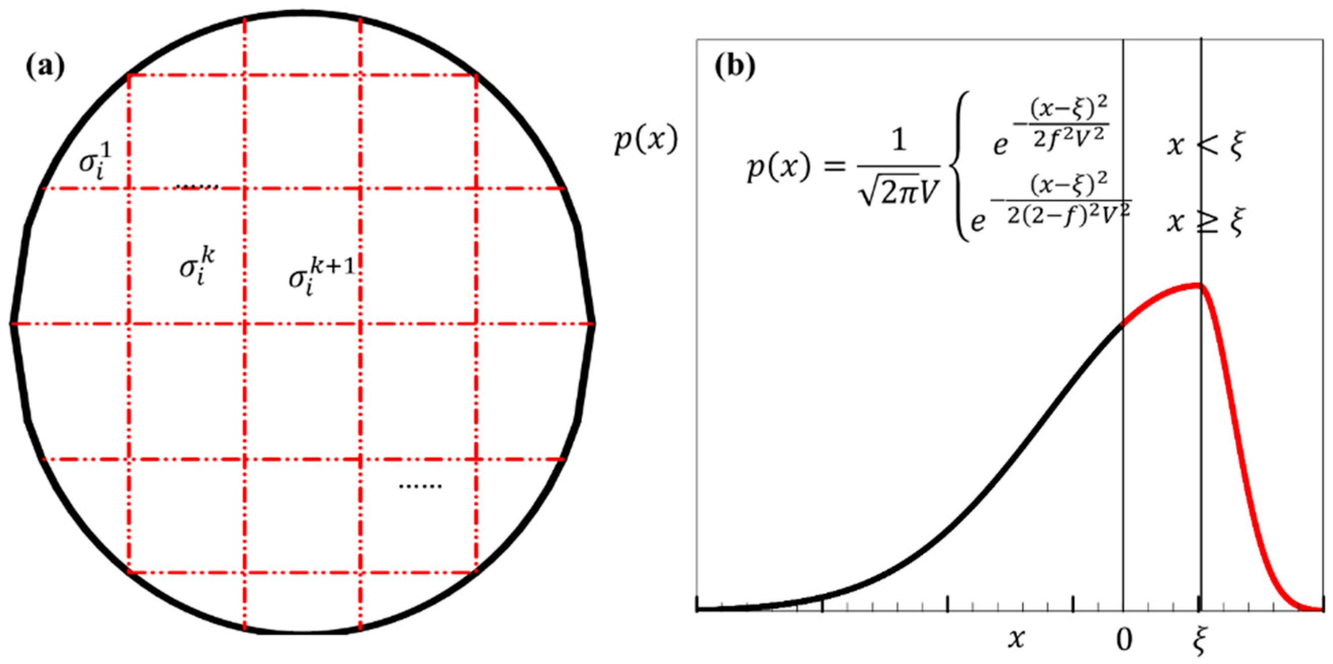
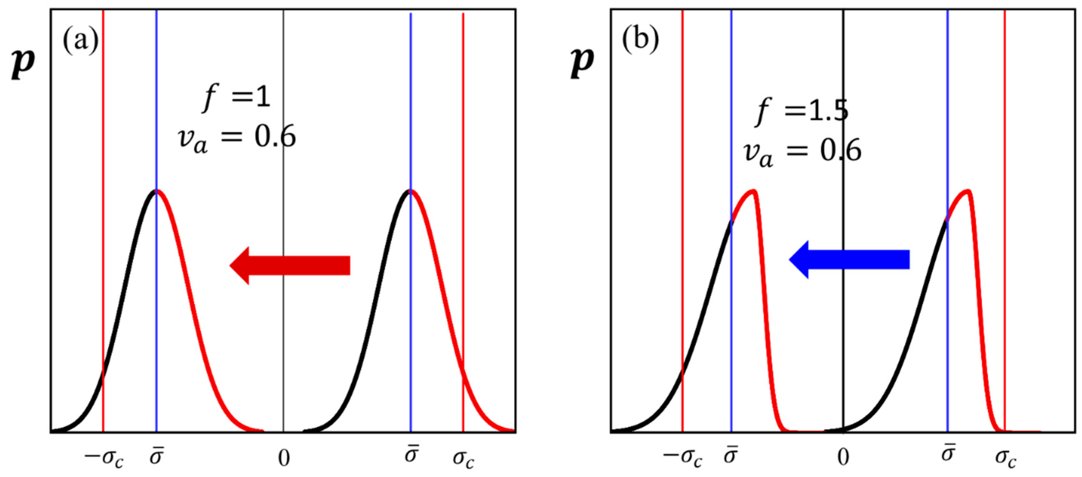
3. Incorporation of the Stress Distribution

The stress state within a material point depends on the density, geometrical arrangement, and interactions of dislocations [21,25,27]. The occurrence of plasticity is attributed to the processes of dislocation unpinning and transport, which rely on the stress state within the activation volume of the unit process. It should be noted that the constitutive law operates at the scale of the material point, which is considerably larger than the activation volume for each activated event. Consequently, the stress state within the material point alone does not provide a complete understanding of the situation, as it fails to account for the fact that the stress in certain subzones is not sufficient to mobilize the dislocations, which causes them to remain immobile, while in others dislocations could be subjected to a higher stress state, for athermal and correlated obstacle bypass [28].

In the present study, the material point is divided into subzones, each having different volumes and stress levels (Figure 1a). The overall stress distribution within a given material point reproduces the stress fluctuations resulting from collective interactions between dislocation segments. Assume that the stress state within a given subzone is denoted by ${\sigma }_i$ and the average stress state within a material point is denoted by ${\overline{\sigma }}_i$. Differentiating between the average stress at the material point and the stress fluctuations at smaller scales is the fundamental rationale behind micro-morphic approaches [29,30]. In the proposed methodology, the probability distribution function (PDF) of the stress state within the material point does not necessarily exhibit symmetrical characteristics. Numerous experiments and models of diffraction line broadening indicate that, in cases where there is no significant contrast in the dislocation distribution within the coherent diffraction domain, Gaussian distributions can be employed to fit the diffraction line profiles. However, when such conditions are not met, the diffraction peak may deviate from symmetry and an asymmetric distribution offers a better fit to experimental data. In the current work, the stress distribution is assumed to be

$${\sigma }_i\left(x\right)={\overline{\sigma }}_i+x{\overline{\sigma }}_i$$

(14)

where x is a scalar to characterize the stress distribution within a material point. The corresponding von Mises stress is ${\sigma }_e\left(x\right)=\left|1+x\right|{\overline{\sigma }}_e$. The fraction of the subzones that have the ${\sigma }_i\left(x\right)$ stress is therefore described by the PDF of x, $p\left(x\right)$. The PDF, not necessarily symmetric, can be expressed as two reformed Gaussian distributions with one reshaped by a factor of $f$ ($0<f<2$) and the other by $\left(2-f\right)$,

$$p\left(x\right)={\displaystyle \frac{1}{\sqrt{2\pi }V}}\left\{\begin{array}{cc}\exp \left(-{\displaystyle \frac{{\left(x-\xi \right)}^2}{2f^2{V}^2}}\right)& x<\xi \\ \exp \left(-{\displaystyle \frac{{\left(x-\xi \right)}^2}{2{\left(2-f\right)}^2{V}^2}}\right)& x\ge \xi \end{array}\right.$$

(15)

where $\xi$, $V$, and $f$ are parameters to define the mean, standard deviation, and shape of the asymmetric stress distribution (Figure 1b). $\xi$ and $V$ have the relation of $\xi ={\displaystyle \frac{4\sqrt{2}}{\sqrt{\pi }}}\left(f-1\right)V$ (see Appendix A). Of course, the asymmetric distribution of the stress will be reduced to symmetric if $f=1$. As learned from [16], the standard deviation of the stress fluctuation $V$ is closely related to the dislocation density as follows:

$$V{\overline{\sigma }}_e=v_{\alpha }\mu b\sqrt{\rho }$$

(16)

where $v_{\alpha }$ is the coefficient used to tune the value of $V$.

According to Equations (3) and (14), the plastic strain rate associated with ${\sigma }_i\left(x\right)$ is

$${\stackrel{·}{\epsilon }}_i^p\left(x\right)={\stackrel{·}{\epsilon }}_e^p\left(\left|1+x\right|{\overline{\sigma }}_e\right){\displaystyle \frac{3{\overline{\sigma }}_i}{2{\overline{\sigma }}_e}}\left(i=1,\dots ,5\right)$$

(17)

The plastic strain rate of the material point is integral of the ${\stackrel{·}{\epsilon }}_i^p\left(x\right)$ over all the distributed stress. This fraction is directly given by the PDF, $p\left(x\right)$, of the stress state. Therefore, the one has the following:

$${\stackrel{·}{\overline{\epsilon }}}_i^p=\int {\stackrel{·}{\epsilon }}_i^p\left(x\right)p\left(x\right)dx$$

(18)

The calculation of the integral employs the Gauss–Legendre quadrature method. By combining Equations (1), (17) and (18), the TST-continuum model is effectively extended to incorporate the stress fluctuation within a material point. In a comprehensive manner, the model proposed in this study is founded upon the J2 plasticity theory utilizing the classical yield surface equation of ${\sigma }_e-{\sigma }_Y=0$. The proposed model can readily accommodate more intricate yielding surfaces to describe the complex deformation behavior of materials.

In this study, the Gauss–Legendre quadrature method is employed to evaluate the plastic strain rate by integrating over the distributed stress (Equation (18)). The choice of Gauss-Legendre quadrature is motivated by its computational efficiency and accuracy, especially in handling integrals with smooth functions like the stress distribution function used in this model. One of the key advantages of the Gauss-Legendre quadrature method is that it allows for high precision with fewer quadrature points compared to other numerical integration methods. This significantly reduces the computational cost when solving the integral of the plastic strain rate over the probability distribution function of stress fluctuations. In our simulations, we found that using a small number of quadrature points (typically around 10 to 20 points) achieves a balance between computational efficiency and accuracy. However, the computational time can be further optimized by adjusting the number of quadrature points based on the complexity of the stress distribution. For more complex or highly nonlinear distributions, increasing the number of quadrature points ensures higher accuracy, but at the expense of additional computational time. Conversely, for simpler distributions, fewer points may suffice, leading to faster computation times.

4. Results and Discussion

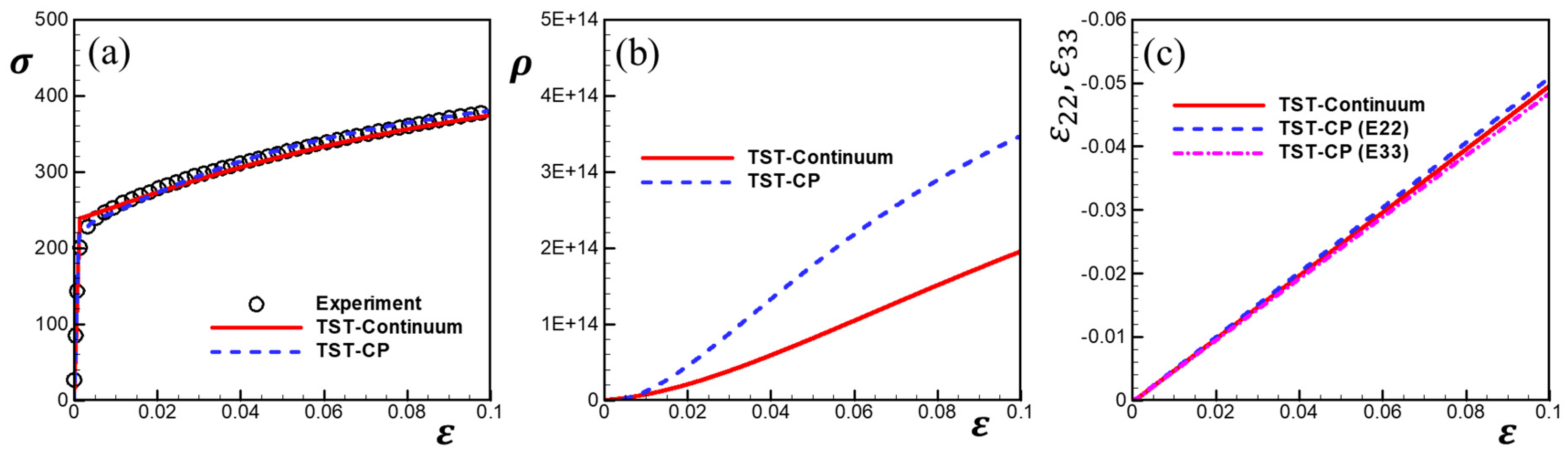
4.1. Unixail Tension

The present study utilized the 316 L austenitic stainless steel, which was previously investigated by Wang et al. [14] and Guo et al. [5]. Figure 2 displays the {111}, {200}, and {220} pole figures of the initial texture, indicating that the as-received stainless steel exhibits a random texture. Due to the high symmetry of the FCC crystallographic structure, the material shows nearly isotropic behavior.

Three experiments were conducted at room temperature to investigate the influence of stress relaxation and strain creep on mechanical behavior. The first experiment involved a uniaxial tension test. The second experiment consisted of conducting a uniaxial tension test with strain-controlled holdings during measurement periods. This setup facilitated the clear observation of stress relaxation in the macroscopic stress–strain response during holding. The third experiment entailed a uniaxial tension test with stress-controlled holdings, leading to the observation of creep during the holding durations. In the interrupted holdings tests, the strain holds occurred at a loading rate of 1 × 10⁻⁴/s, and each holding lasted for 15 min (900 s).

The experimental results are modeled using the TST-continuum model, disregarding stress distribution (referred to as Equation (14)), and are compared to the simulated outcomes obtained with the crystal plasticity model based on the transition state theory (abbreviated as TST-CP). The parameters associated with the TST-continuum model used in this study are determined by fitting the uniaxial stress–strain curve (

Table 1. Values of the parameters used in the TST-continuum model.

K1 (m−1)	D (MPa)	g	ΔG (eV)	σ0 (MPa)	E (GPa)	ν	T (°K)
4.4 × 108	100	0.07	7	305	180	0.29	298
m	n	νa	ρ0 (m−2)	b (Å)	α	M	vs (m/s)
2/3	3/2	0	1.2 × 1012	2.546	0.3	3.06	1500

). The simulation employs a boundary condition for uniaxial loading, with ${\stackrel{·}{\sigma }}_{ij}=0$, except for ${\stackrel{·}{\sigma }}_{11}>0({\stackrel{·}{\epsilon }}_{11}={10}^{-4}{\mathrm{s}}^{-1})$. Figure 3a depicts the fitted monotonic stress–strain curve, coinciding well with the experimental curve. Moreover, the stress–strain curve obtained through the TST-CP is included in Figure 3a, exhibiting consistency with the TST-continuum result. In addition, Figure 3b presents the predicted dislocation densities alongside the stress–strain curves. The predicted dislocation density is approximately ${10}^{14}{\mathrm{m}}^{-2}$, showing consistency with predictions obtained from the TST-CP model and experimental observations [16]. The slight quantitative disparity between the two models is reasonable due to the comprehensive consideration of all constituted dislocation slip systems in the CP model. Conversely, the TST-continuum model characterizes the hardening behavior of the material through an effective dislocation density. Under uniaxial tension, the isotropic nature of the TST-continuum model results in identical lateral strain components ${\epsilon }_{22}$ and ${\epsilon }_{33}$, which are compared to the corresponding predictions of the TST-CP model in Figure 3c. The close proximity between the strain components ${\epsilon }_{22}$ and ${\epsilon }_{33}$ provides evidence of the nearly isotropic behavior exhibited by the investigated stainless steel. Additionally, the computational cost of the TST-continuum model is significantly lower compared to the TST-CP model. The TST-continuum calculation only requires approximately 0.1 s of CPU time, while the TST-CP calculation for 23,328 grains takes around 3 h. The computational cost saving achieved by the TST-continuum model is on the order of ${10}^5$, which is comparable to the product of the number of grains ($2\times {10}^4$) and the number of slip systems (12) considered in the CP simulation.

The loading cases of uniaxial compression, axisymmetric compression, and simple shear are simulated by both the TST-continuum and TST-CP. The boundary condition for uniaxial compression is ${\stackrel{·}{\sigma }}_{ij}=0$, except ${\stackrel{·}{\sigma }}_{11}<0$ $({\stackrel{·}{\epsilon }}_{11}=-{10}^{-4}{\mathrm{s}}^{-1})$. The stress–strain response and the corresponding lateral strain components are compared in Figure 4a and Figure 4b, respectively. The TST-continuum model can reasonably reproduce the results obtained by the TST-CP. The boundary condition for axisymmetric compression is ${\stackrel{·}{\epsilon }}_{ij}=0$, except ${\stackrel{·}{\epsilon }}_{11}=-2{\stackrel{·}{\epsilon }}_{22}=-2{\stackrel{·}{\epsilon }}_{33}=-{10}^{-4}{\mathrm{s}}^{-1}$. The evolution of the major stress component ${\sigma }_{11}$, and lateral stress components ${\sigma }_{22}$ and ${\sigma }_{33}$ as a function of the applied strain are presented in Figure 5a. The results produced by the TST-continuum are consistent with those obtained by the TST-CP. Again, the nearly isotropic behavior of stainless steel is observed from the close lateral strain components ${\epsilon }_{22}$ and ${\epsilon }_{33}$. The boundary condition for plane strain compression is ${\stackrel{·}{\epsilon }}_{11}=-{10}^{-4}{\mathrm{s}}^{-1}$, ${\stackrel{·}{\epsilon }}_{12}={\stackrel{·}{\epsilon }}_{23}={\stackrel{·}{\epsilon }}_{31}={\stackrel{·}{\epsilon }}_{22}=0$, and ${\stackrel{·}{\sigma }}_{33}=0$. The evolution of the stress components ${\sigma }_{11}$ and ${\sigma }_{22}$ as a function of the applied strain is presented in Figure 5b. The boundary condition for simple shear is ${\stackrel{·}{\epsilon }}_{ij}=0$ except for ${\stackrel{·}{\epsilon }}_{12}={\stackrel{·}{\epsilon }}_{21}={10}^{-4}{\mathrm{s}}^{-1}$. The shear stress and shear strain curves produced by the two models are in good agreement (Figure 6). The good match for different loading cases indicates that the TST-continuum model can reproduce well the macroscopic mechanical behaviors obtained from the TST-CP.

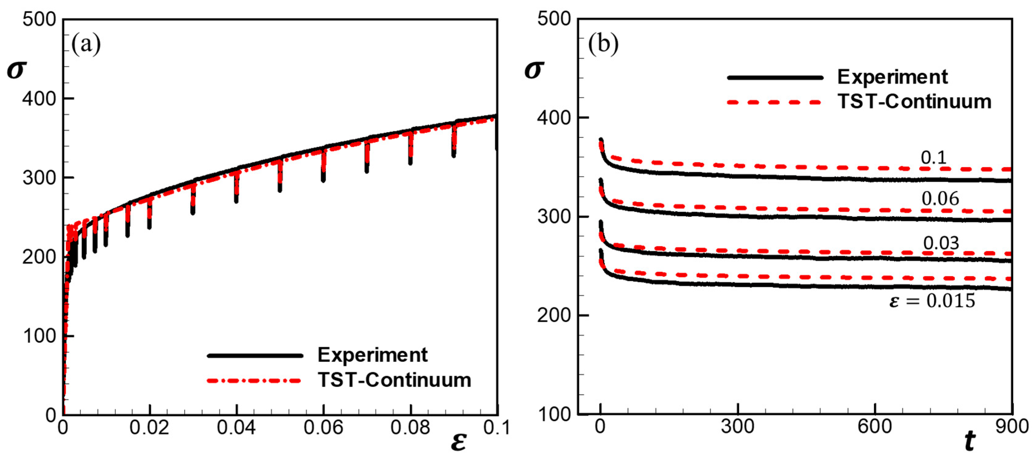
4.2. Loading with Stress Holds

By employing the TST-continuum model, the tests with strain holds and stress holds are simulated by the proposed model, which, respectively, represent the cases of strain creep and stress relaxation. During the strain creep simulation, the boundary condition maintains a constant applied stress of ${\stackrel{·}{\sigma }}_{ij}=0$ for a creep time interval of 900 s. Subsequently, a strain rate of ${10}^{-4}{\mathrm{s}}^{-1}$ is applied until reaching the next holding point. The stress–strain curves and the development of strains over time during stress holding are presented in Figure 7a,b. Notably, clear strain plateaus (creep section) are observed during each stress-controlled holding period. Throughout each holding stage, the increase in threshold stress, caused by stored dislocations, results in its displacement away from the von Mises stress criterion. This displacement reduces the probability of dislocation segments becoming unpinned (i.e., a smaller plastic strain rate).

4.3. Loading with Strain Holds

To simulate the loading with strain holds, the total strain is held constant for 900 s. Subsequently, a strain rate of ${10}^{-4}{\mathrm{s}}^{-1}$ is applied until reaching the next holding point. During the holding period, the boundary condition is as follows: ${\stackrel{·}{\epsilon }}_{11}=0$, ${\stackrel{·}{\sigma }}_{ij}=0$ except ${\stackrel{·}{\sigma }}_{11}\ne 0$, where ${\sigma }_{11}$ represents the only non-zero stress component in tension. In Figure 8a, a comparison is shown between the simulated stress–strain curve with strain holdings and the experimental data. The stress evolution within the strain holdings is illustrated in Figure 8b, demonstrating the occurrence of stress drops (stress relaxation) during each strain-controlled holding. This phenomenon arises from the reduction in stress during each holding period, causing the von Mises stress to move away from the threshold stress. As a result, the likelihood of dislocation segments becoming dislodged decreases (resulting in a smaller plastic strain rate).

Figure 7 and Figure 8 indicate that the TST-continuum model interprets well the amount and time dependence of the strain crept during stress holding and the stress dropped during strain holding.

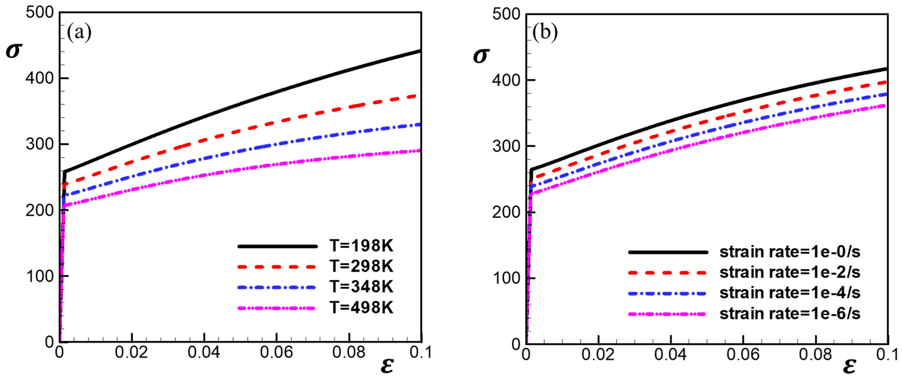
4.4. Dependency of Temperature and Strain Rate

By being grounded in the harmonic transition state theory (TST), the TST-continuum model has the capability to replicate the impacts of both temperature and strain rate on the mechanical properties of materials. In Figure 9a, simulated stress–strain curves are presented for temperatures of 198 K, 298 K, 398 K, and 498 K. Notably, the TST-continuum model effectively captures the correlation between lower temperatures and enhanced flow stress. This increase in flow stress with temperature aligns with the findings reported by Wang et al. [15] for 304 stainless steel.

To investigate the influence of strain rate, the mechanical response of stainless steel under tension is simulated at strain rates of 1.0, ${10}^{-2}$, ${10}^{-4}$, and ${10}^{-6}$ $s^{-1}$ (Figure 9b). The strain rate sensitivity, as determined by the value of ${\displaystyle \frac{kT}{\Delta G_0}}$ from Equation (15), enhances with higher strain rates, resulting in increased stress and a steeper hardening rate. Consequently, the rate sensitivity of the material is governed by the dislocation activation energy $\Delta G_0$ and temperature T, wherein lower activation energy or higher temperature leads to higher rate sensitivity. The findings reveal that 316 L stainless steel exhibits a consistently low rate sensitivity, which is consistent with previous experimental observations [31].

In addition to the aforementioned cases, simulations were performed considering stress fluctuation, yielding similar results with only minor quantitative discrepancies (as shown in Figure 10). The successful simulation of these monotonic cases highlights the effectiveness of the proposed TST-continuum model. Nevertheless, practical applications frequently involve intricate loadings that incorporate the Bauchinger effect during strain path reversals. Accounting for this effect is crucial for accurate constitutive modeling.

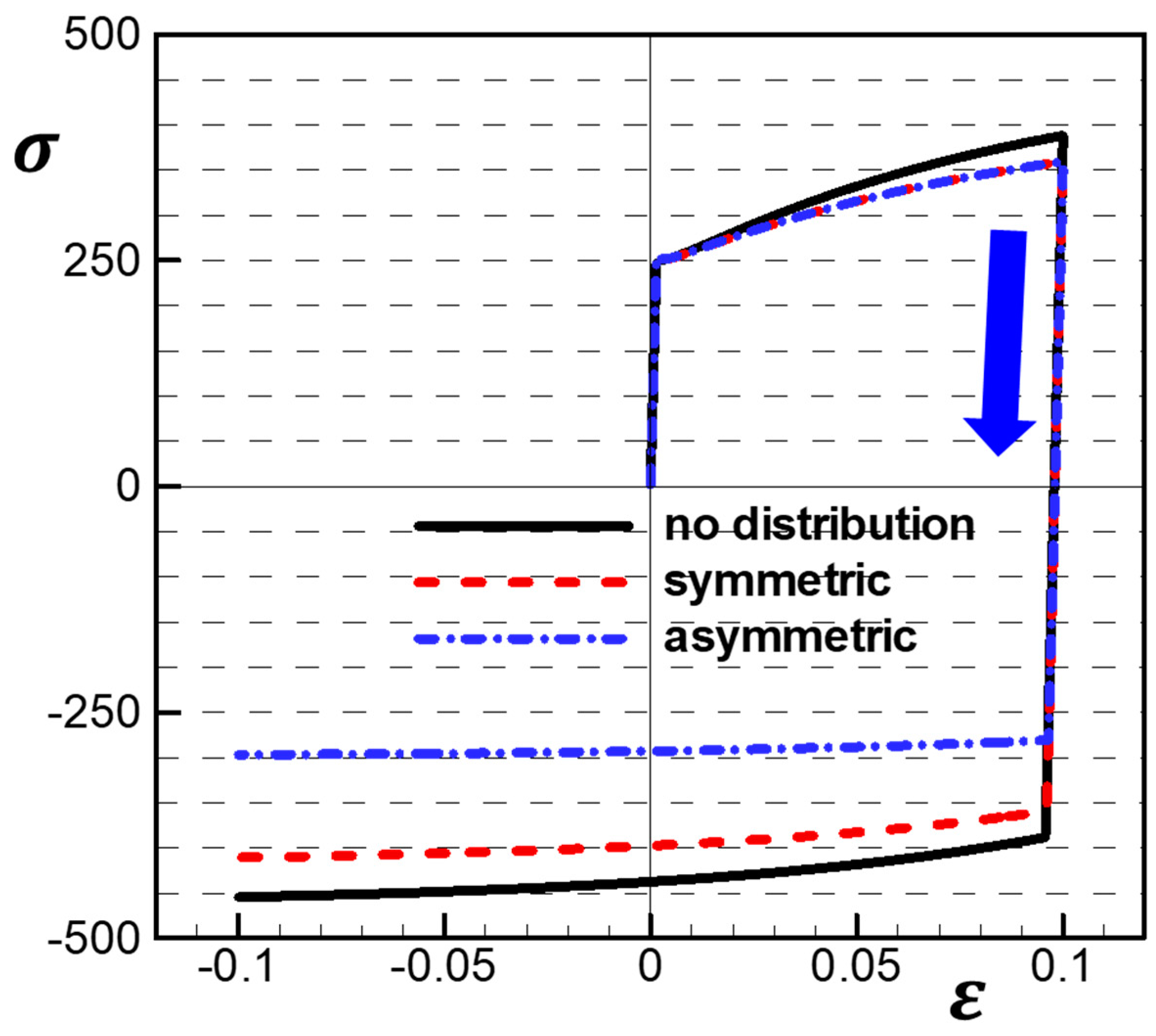
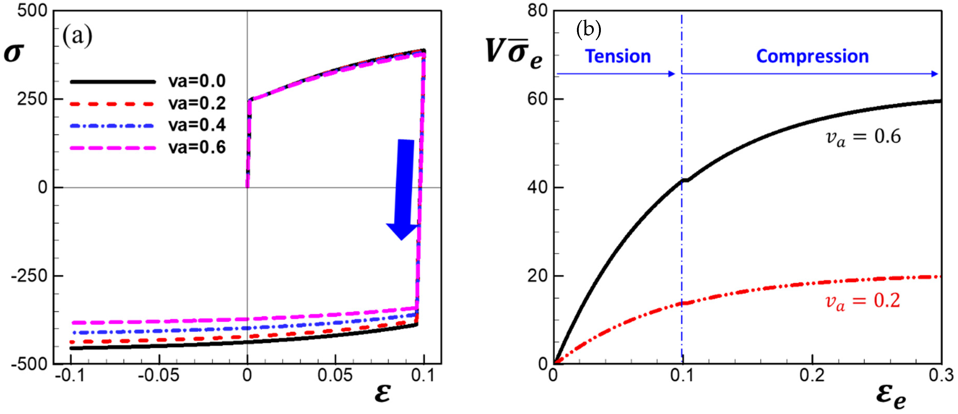
4.5. The Bauschinger Effect

The Bauchinger effect refers to the requirement of a lower yielding strength to accommodate plastic strain during reverse loading compared to unloading. Traditional constitutive models commonly incorporate back-stress to address this phenomenon. As mentioned earlier, a representative metallic material point can consist of numerous grains, each potentially subjected to distinct stress levels. In this section, the TST-continuum model is utilized to consider the inherent stress fluctuation within a material point, thereby accurately characterizing the Bauchinger effect during a reversal in the loading path. Consequently, the TST-continuum model is employed to simulate a tension-loading scenario followed by compression, taking into account the influence of stress fluctuation.

In the simulations, both symmetric and asymmetric stress distributions are taken into consideration. Figure 11 presents a comparison of the simulated stress–strain curves for cyclic tension and compression, considering symmetric stress distribution ($f=1.0$), asymmetric stress distribution ($f=1.5$) with a stress distribution $v_{\alpha }=0.6$, and the absence of stress distribution ($V=0$). Under both forward tension and backward compression, the flow stress magnitude is reduced when incorporating either symmetric or asymmetric stress distribution. In simpler terms, when the stress fluctuates within the material point, more deformation is induced compared to a homogeneous stress state. The TST-continuum model, without accounting for stress distribution or with symmetric stress distribution, fails to replicate the Bauchinger effect. This outcome was expected since the model does not differentiate the yielding strength under tension and compression. However, the TST-continuum model, incorporating asymmetric stress distribution, successfully captures the Bauchinger effect during loading reversal. This finding aligns with experimental observations for 317 L stainless steel [32,33]. Figure 12 presents a schematic illustration of the evolution of symmetric and asymmetric stress distributions. Prior to yielding during reverse compression, the threshold stress ${\sigma }_c$ remains consistent with the loading reversal. In cases where symmetric or no stress distribution is considered (Figure 12a), the same stress magnitude is required to accommodate plastic deformation at the points of loading reversal and compressive yielding. Conversely, in the presence of asymmetric stress distribution (Figure 12b), a lower average stress $\overline{\sigma }$ is needed to accommodate plastic strain, which corresponds to the Bauchinger effect. The reasonable nature of the asymmetric stress distribution depicted in Figure 12b arises from the instantaneous unpinning of dislocations with $\sigma \ge {\sigma }_c$. In essence, the appropriate range for stress dispersion is $\left(-{\sigma }_c,\overline{\sigma }\right)$ on the left side of the distribution and $\left(\overline{\sigma },{\sigma }_c\right)$ on the right. For instance, as the average stress $\overline{\sigma }>0$ approaches the critical value ${\sigma }_c$, the right side of the distribution gradually becomes narrower. Consequently, the shape of the stress distribution evolves to be non-symmetric (Figure 12b). Upon reversing the loading, the decrease in average stress does not significantly alter the shape of the distribution until its magnitude is comparable to the threshold value $-{\sigma }_c$. Consequently, plastic deformation occurs earlier at a yielding stress (absolute value) smaller than the stress observed during the loading reversal, exemplifying the Bauchinger effect. The shape of the probability distribution function evolves with the amount of dislocation density. While the current work treats the parameter $f$ as constant, it is important to note that $f$ evolves as a function of the loading history, including the stress ${\sigma }_i$ and the dislocation density $\rho$.

In the TST-continuum model, the magnitude of the Bauchinger effect can be adjusted. This tunability is demonstrated by variations in the factor $v_a$, which directly influences the standard deviation of the stress distribution $V$. Figure 13a illustrates the simulated stress–strain curves for different values of $v_a$. Notably, Figure 13b reveals that the standard deviation $V$ is not a constant throughout the deformation process. Instead, it progressively increases with the accumulated strain during tension compression, as updated according to Equation (17).

5. Conclusions

A continuum plasticity model based on both the dislocation theory and the transition state theory is developed for metallic materials. Furthermore, the stress distribution is accounted for by introducing a probability distribution function to resemble the stress fluctuation within a material point. The model is applied to study the mechanical behavior of 316 L stainless steel under various loading conditions and a good agreement has been obtained. As demonstrated, this work provides an alternative and efficient model in the investigation of the behaviors of metallic materials. The following conclusions can be drawn:

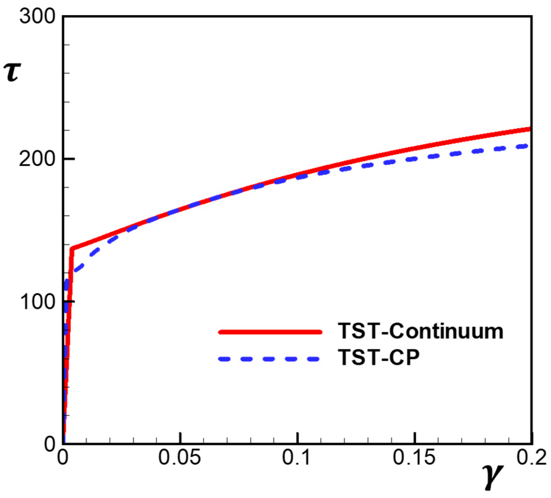
• The model adequately describes the mechanical behaviors of materials and reproduces the results obtained by the polycrystal plasticity model. The computational time savings are on the order of the product of the number of grains and the number of systems considered;
• The strain rate sensitivity of a material is taken into account in terms of its dependence on the dislocation activation energy. As a consequence, the effects of stress relaxation and strain creep are correctly captured by the model;
• The temperature dependence of material is also taken into account in terms of the harmonic transition state theory. Higher flow stress and higher hardening rate are obtained with lower temperature, which is consistent with the experimental observations;
• The model is further enhanced by accounting for the stress distribution. By incorporating an asymmetric stress distribution, the model captures the Bauschinger effect, which is not accounted for by a conventional continuum model without additional treatment.

References

1. Ni, R.; Boehlert, C.J.; Zeng, Y.; Chen, B.; Huang, S.; Zheng, J.; Zhou, H.; Wang, Q.; Yin, D. Automated Analysis Framework of Strain Partitioning and Deformation Mechanisms via Multimodal Fusion and Computer Vision. Int. J. Plast. 2024, 182, 104–119. [Google Scholar] [CrossRef]
2. McDowell, D.L. Viscoplasticity of heterogenous metallic materials. Mater. Sci. Emg. R Rep. 2008, 62, 67–123. [Google Scholar] [CrossRef]
3. Chaboche, J.L. A review of some plasticity and viscoplasticity constitutive theories. Int. J. Plast. 2008, 24, 1642–1693. [Google Scholar] [CrossRef]
4. Drucker, D.C.; Prager, W. Soil mechanics and plastic analysis of limit design. Q. Appl. Math. 1952, 10, 157–162. [Google Scholar] [CrossRef]
5. Guo, X.Q.; Wu, P.D.; Wang, H.; Mao, X.B. Study of lattice strain evolution in stainless steel under tension: The role of self-consistent plasticity model. Steel Res. Int. 2015, 86, 894–901. [Google Scholar] [CrossRef]
6. Gurson, A.L. Continuum Theory of Ductile Rupture by Void Nucleation and Growth: Part I—Yield Criteria and Flow Rules for Porous Ductile Media. J. Eng. Mater. Technol. 1977, 99, 2. [Google Scholar] [CrossRef]
7. Hirth, J.P.; Lothe, J.; Mura, T. Theory of Dislocations. J. Appl. Mech. 1983, 50, 476. [Google Scholar] [CrossRef]
8. Huang, Y.; Qu, S.; Hwang, K.C.; Li, M.; Gao, H. A conventional theory of mechanism-based strain gradient plasticity. Int. J. Plast. 2004, 20, 753–782. [Google Scholar] [CrossRef]
9. Rahaman, M.M.; Dhas, B.; Roy, D.; Reddy, J.N. A dynamic flow rule for viscoplasticity in polycrystalline solids under high strain rates. Int. J. Non-Linear Mech. 2017, 95, 10–18. [Google Scholar] [CrossRef]
10. Orowan, E. Zur Kristallplastizitt. III. Z. Physik 1934, 89, 634–659. [Google Scholar] [CrossRef]
11. Taylor, G.I. The mechanism of plastic deformation of crystals, Part I—Theoretical. Proc. R. Soc. Lond. Ser. A 1934, 145, 362–387. [Google Scholar]
12. Wenk, H.R.; Lutterotti, L.; Vogel, S. Texture analysis with the new HIPPO TOF diffractometer. Nucl. Instrum. Methods Phys. Res. Sect. A Accel. Spectrometers Detect. Assoc. Equip. 2003, 515, 575–588. [Google Scholar] [CrossRef]
13. Wang, H.; Wu, P.D.; Tomé, C.N.; Huang, Y. A finite strain elastic-viscoplastic self-consistent model for polycrystalline materials. J. Mech. Phys. Solids 2010, 58, 594–612. [Google Scholar] [CrossRef]
14. Wang, H.; Wu, P.D.; Tomé, C.N.; Wang, J. A crystal plasticity model for hexagonal close packed (HCP) models including twinning and de-twinning mechanisms. Int. J. Plast. 2013, 49, 36–52. [Google Scholar] [CrossRef]
15. Wang, H.; Clausen, B.; Capolungo, L.; Beyerlein, I.J.; Wang, J.; Tomé, C.N. Stress and strain relaxation in magnesium AZ31 rolled plate: In-situ neutron measurement and elastic viscoplastic self-consistent polycrystal modeling. Int. J. Plast. 2016, 79, 275–292. [Google Scholar] [CrossRef]
16. Wang, H.; Capolungo, L.; Clausen, B.; Tomé, C.N. A crystal plasticity model based on transition state theory. Int. J. Plast. 2017, 93, 251–268. [Google Scholar] [CrossRef]
17. Vineyard, G.H. Frequency factors and isotope effects in solid state rate processes. J. Phys. Chem. Solids 1957, 3, 121–127. [Google Scholar] [CrossRef]
18. Kocks, U.F.; Argon, A.S.; Ashby, M.F. Thermodynamics and Kinetics of Slip. Prog. Mater. Sci. 1975, 19, 171–229. [Google Scholar]
19. Balogh, L.; Ribarik, G.; Ungar, T. Stacking faults and twin boundaries in fcc crystals determined by x-ray diffraction profile analysis. J. Appl. Phys. 2006, 100, 023512. [Google Scholar] [CrossRef]
20. Balogh, L.; Capolungo, L.; Tome, C.N. On the measure of dislocation densities from diffraction line profiles: A comparison with discrete dislocation methods. Acta Mater. 2012, 60, 1467–1477. [Google Scholar] [CrossRef]
21. Ungar, T.; Dragomir, I.; Revesz, A.; Borbely, A. The contrast factors of dislocations in cubic crystals: The dislocation model of strain anisotropy in practice. J. Appl. Crystallogr. 1999, 32, 992–1002. [Google Scholar] [CrossRef]
22. Ungar, T.; Gubicza, J.; Ribarik, G.; Borbely, A. Crystallite size distribution and dislocation structure determined by diffraction profile analysis: Principles and practical application to cubic and hexagonal crystals. J. Appl. Crystallogr. 2001, 34, 298–310. [Google Scholar] [CrossRef]
23. Ungar, T.; Ribarik, G.; Balogh, L.; Salem, A.A.; Semiatin, S.L.; Vaughan, G.B.M. Burgers vector population, dislocation types and dislocation densities in single grains extracted from a polycrystalline commercial-purity Ti specimen by X-ray line-profile analysis. Scr. Mater. 2010, 63, 69–72. [Google Scholar] [CrossRef]
24. Granato, A.; Lücke, K. Theory of mechanical damping due to dislocations. J. Appl. Phys. 1956, 27, 583–593. [Google Scholar] [CrossRef]
25. Wilkens, M. Fundamental Aspects of Dislocation Theory; Simmons, J.A., de Wit, R., Bullough, R., Eds.; Naturnal Bureau of Standards; (US) Special Publication No. 317; United States Department of Commerce: Washington, DC, USA, 1970; Volume II, p. 1195. [Google Scholar]
26. Beyerlein, I.J.; Tomé, C.N. A dislocation-based constitutive law for pure Zr including temperature effects. Int. J. Plast. 2008, 24, 867–895. [Google Scholar] [CrossRef]
27. Besseling, J.F. A theory of elastic, plastic, and creep deformations of an initially isotropic material showing anisotropic strain-hardening, creep recovery, and secondary creep. J. Appl. Mech. 1958, 25, 529–536. [Google Scholar] [CrossRef]
28. Picu, R.C. On the function form of non-local elasticity kernels. J. Mech. Phys. Solids 2002, 50, 1923–1939. [Google Scholar] [CrossRef]
29. Gurtin, M.E. On the plasticity of single crystals: Free energy, microforce, plastic-strain gradient. J. Mech. Phys. Solids 2000, 48, 989–1036. [Google Scholar] [CrossRef]
30. Forest, S. Micromorphic approach for gradient elasticity, viscoplasticity and damage. J. Eng. Mech. 2009, 135, 117–131. [Google Scholar] [CrossRef]
31. Talyan, V.; Wagoner, R.H.; Lee, J.K. Formability of stainless steel. Metall. Mater. Trans. A 1998, 29, 2161–2172. [Google Scholar] [CrossRef]
32. Wollmershauser, J.A.; Clausen, B.; Agnew, S.R. A slip system-based kinematic hardening model application to in situ neutron diffraction of cyclic deformation of austenitic stainless steel. Int. J. Fatigue 2012, 36, 181–193. [Google Scholar] [CrossRef]
33. Cebrian, C.A.; Zaki, W. Fatigue of Shape Memory Alloys with Emphasis on Additively Manufactured NiTi Components. Appl. Mech. Rev. 2022, 74, 040801. [Google Scholar] [CrossRef]
Figure 1. Schematic representation of the distribution of the stress in a material point: (a) different stresses in different subzones; (b) probability distribution function of stress within the material point.
Metals 14 01228 g001
Figure 2. {111}, {200}, {220} pole figures of the initial texture. Reprinted from Ref. [14].
Metals 14 01228 g002
Figure 3. (a) Experimental and simulated stress–strain curves under uniaxial tension; (b) simulated dislocation densities; and (c) simulated lateral strain ε22 and ε33.
Metals 14 01228 g003
Figure 4. (a) Simulated stress–strain curves under uniaxial compression; (b) simulated lateral strain components ε 22 and ε 33 .
Metals 14 01228 g004
Figure 5. Simulated stress–strain curves under (a) axisymmetric compression, and (b) plane strain compression.
Metals 14 01228 g005
Figure 6. Simulated shear stress–shear strain curves under simple shear.
Metals 14 01228 g006
Figure 7. (a) simulated stress–strain curves under tension with stress holding, and (b) strain evolution during strain holding at different holding stresses.
Metals 14 01228 g007
Figure 8. (a) Simulated stress–strain curves under tension with strain holding, and (b) stress evolution during strain holding at different holding strains.
Metals 14 01228 g008
Figure 9. Simulated stress–strain curves of the 316 L stainless steel under monotonic tension at (a) a temperature of 298 K and strain rates of 1.0   s 1 , 10 2 s 1 , 10 4 s 1 , and 10 6 s 1 ; and (b) a strain rate of 1 × 10 4 s 1 and temperatures of 198 K, 298 K, 398 K, and 498 K.
Metals 14 01228 g009
Figure 10. Simulated stress–strain curves of the 316 L stainless steel under tension with and without stress fluctuation.
Metals 14 01228 g010
Figure 11. Simulated stress–strain curves under cyclic tension and compression with symmetric and asymmetric stress distributions.
Metals 14 01228 g011
Figure 12. Schematic representation of the evolution of (a) symmetric stress distribution; and (b) asymmetric stress distribution.
Metals 14 01228 g012
Figure 13. (a) Simulated stress–strain curves under tension followed by compression with asymmetric stress distribution; (b) The evolution of the value V as a function of accumulated strain under tension compression.
Metals 14 01228 g013