Improved YOLOv5 Network for Steel Surface Defect Detection

Abstract

Steel surface defect detection is crucial for ensuring steel quality. The traditional detection algorithm has low detection probability. This paper proposes an improved algorithm based on the YOLOv5 model to enhance detection probability. Firstly, deformable convolution is introduced in the backbone network, and a traditional convolution module is replaced by deformable convolution; secondly, the CBAM attention mechanism is added to the backbone network; then, Focal EIOU is used instead of the CIOU loss function in YOLOv5; lastly, the K-means algorithm is used to cluster the Anchor box, and the Anchor box parameters that are more suitable for this paper are obtained. The experimental results show that using deformable convolution instead of traditional convolution can get more feature information, which is more conducive to the learning of the network. This paper uses the CBAM attention mechanism, and the heat map of the attention mechanism shows that the CBAM attention mechanism is beneficial for feature extraction. Focal EIOU is optimized in high and wide loss compared with the CIOU loss function, which accelerates the convergence of the model. The Anchor box is more favorable for feature extraction. The improved algorithm achieved a detection probability of 78.8% in the NEU-DET dataset, which is 4.3% better than the original YOLOv5 network, and the inference time of each image is only increased by 1 ms; therefore, the optimized algorithm proposed in this paper is effective.

1. Introduction

As an important metal resource, steel is one of the main industrial materials. Due to the production process, cracks, patches, scratches and other defects inevitably appear during the production process. These defects affect the aesthetics of steel; at the same time, the corrosion resistance and wear resistance of steel are affected due to the surface defects, thereby reducing its service life.

The traditional inspection method for defect detection in the industry is manual visual inspection, which is susceptible to visual fatigue. In recent years, with the rapid development of computer vision, visual inspection, instead of the traditional manual approach, has become mainstream in quality inspection. Defect detection belongs to the category of surface detection, which has been studied by many scholars [1,2,3], including the aspects of texture features, color features, and shape features, which summarize the application of traditional vision in surface defect detection.

In terms of machine vision technology, along with the continuous progress of computer hardware, the deep learning algorithm has become the mainstream inspection algorithm because of its simple and efficient network structure to obtain higher detection probability and faster detection speed than traditional algorithms. The authors of [4] proposed a convolutional neural network method for automatically detecting surface defects on workpieces. The feature extraction and loss function were optimized, three convolutional branches of the FPN (feature pyramid network) structure were used for feature recognition, and the detection performance was significantly improved. In addition to surface defects, internal defects of steel are critical to the quality of steel. Various internal defects commonly found in CFRP (carbon fiber-reinforced polymer)-reinforced steel structures were studied in [5]. The effectiveness of eddy current pulse thermography (ECPT) for detecting internal defects in CFRP reinforced steel structures was explored. The study proposed a defect detection and classification method for OSC (organic solar cells). Image features were extracted using Zernike moments, and different defects were classified using EBFNNs (elliptical basis function neural networks); the detection probability reached 89%, as verified by experiments [6].

SSD and YOLOv5 are representative algorithms for single-stage target detectors. Researchers have used YOLOv5 to detect steel weld defects [7]. An improved single-stage target detector called a multi-scale feature cross-layer fusion network (M-FCFN) was proposed in [8]; shallow features and deep features were extracted from the PANet (path aggregation network) structure for cross-layer fusion, and the loss function was optimized. The optimized network showed some improvement in detection probability. The ACP-YOLOv3-dense (classification priority YOLOv3 DenseNet) neural network was proposed in [9]. The model used YOLOv3 as the base network to prioritize images for classification, and then replaced two residual network modules with two dense network modules. The results showed that the detection probability was improved compared to before optimization.

The authors of [10] proposed the DF-ResNeSt50 network model, based on the visual attention mechanism in the bionic algorithm, by combining the feature pyramid network and split-attention network model and optimizing them from the perspectives of data enhancement, multi-scale feature fusion, and network structure optimization. The detection performance and detection efficiency were improved. In [11], a YOLOv5 algorithm with a fused attention mechanism was proposed, which used the backbone network for feature extraction and fused the attention mechanism to represent different features so that the network could fully extract the texture and semantic features of the defective region; the CIOU loss function was used instead of the GIOU loss function. The improved network could identify the location and class of defects more accurately. The authors of [12] addressed the traditional target detection methods that cannot effectively filter key features, leading to overfitting of the model and weak generalization ability. An improved SE-YOLOv5 network model was proposed. The average accuracy was effectively improved by adding the SE module to the YOLOv5 model.

The authors of [13] proposed a method that combined an improved ResNet50 with an enhanced, faster regional convolutional neural network (faster R-CNN) to reduce the average running time and improve the accuracy. An accuracy of up to 98.2% was achieved on the steel dataset created by the authors. The authors of [14] created a hot-rolled strip steel surface defect dataset (X-SDD) using the newly proposed RepVGG algorithm. It was combined with the spatial attention (SA) mechanism to verify the impact on X-SDD. The test results showed that the algorithm achieved an accuracy of 95.10% on the test set. In [15], an automatic detection and classification method for rolling metal surface defects was proposed, which could perform defect inspection with specified efficiency and speed parameters. According to the test data, the model could classify planar damage images into three categories with an overall accuracy of 96.91%.

Lightweight networks are also among the current research focuses, and an enhanced lightweight YOLOv5 (MR-YOLO) method was proposed in [16] to identify magnetic ring surface defects. The Mobilenetv3 module was added to the YOLOv5 neck network, a mosaic data enhancement technique was used, and the SE attention module was inserted in the backbone network to optimize the loss function. The FLOP and Params of the improved network model decreased significantly, the inference speed increased by 16.6%, the model size decreased by 48.1%, and the mAP decreased by only 0.3%.

The authors of [17] performed detection on the NEU-DET dataset by reconstructing the network structure of faster R-CNN. A multi-scale fusion training network was used for the target’s small features. For the complex features of the target, a deformable convolutional network was used instead of part of the traditional convolutional network. The final average accuracy was 0.752, which was 0.128 better than the original algorithm. The authors of [18] proposed a method for training neural network vision tasks on the basis of comprehensive data. The neural network achieved good results for both the classification and the segmentation of surface defects of steel workpieces in images. The study showed the possibility of training deep neural networks using synthetic datasets.

In target detection, external noise has a great impact on the detection results of the image; reasonable denoising and removal of irrelevant background can play good roles in detection. Some authors introduced the visual attention mechanism into sparse representation classification and proposed a weighted block collaborative sparse representation method based on a visual saliency dictionary. Data redundancy was reduced, and the region of interest was better focused. The sparse coding of different local structures of the face achieved better results in face recognition [19]. The authors proposed a network of HDCNN in which DB (a dilated block), RVB (a dilated block), and FB (feature refinement block) were introduced into the CNN to enhance the denoising ability of the network. Experiments showed that the network achieved good denoising results on the dataset [20]. The researchers proposed a comparative sample-enhanced image drawing strategy that improved the quality of the training set by filtering irrelevant images and constructing additional images using information from the region surrounding the target image; it effectively solved the problem of differences in the quality of image drawing due to differences in the size and diversity of the underlying training data in different contexts [21].

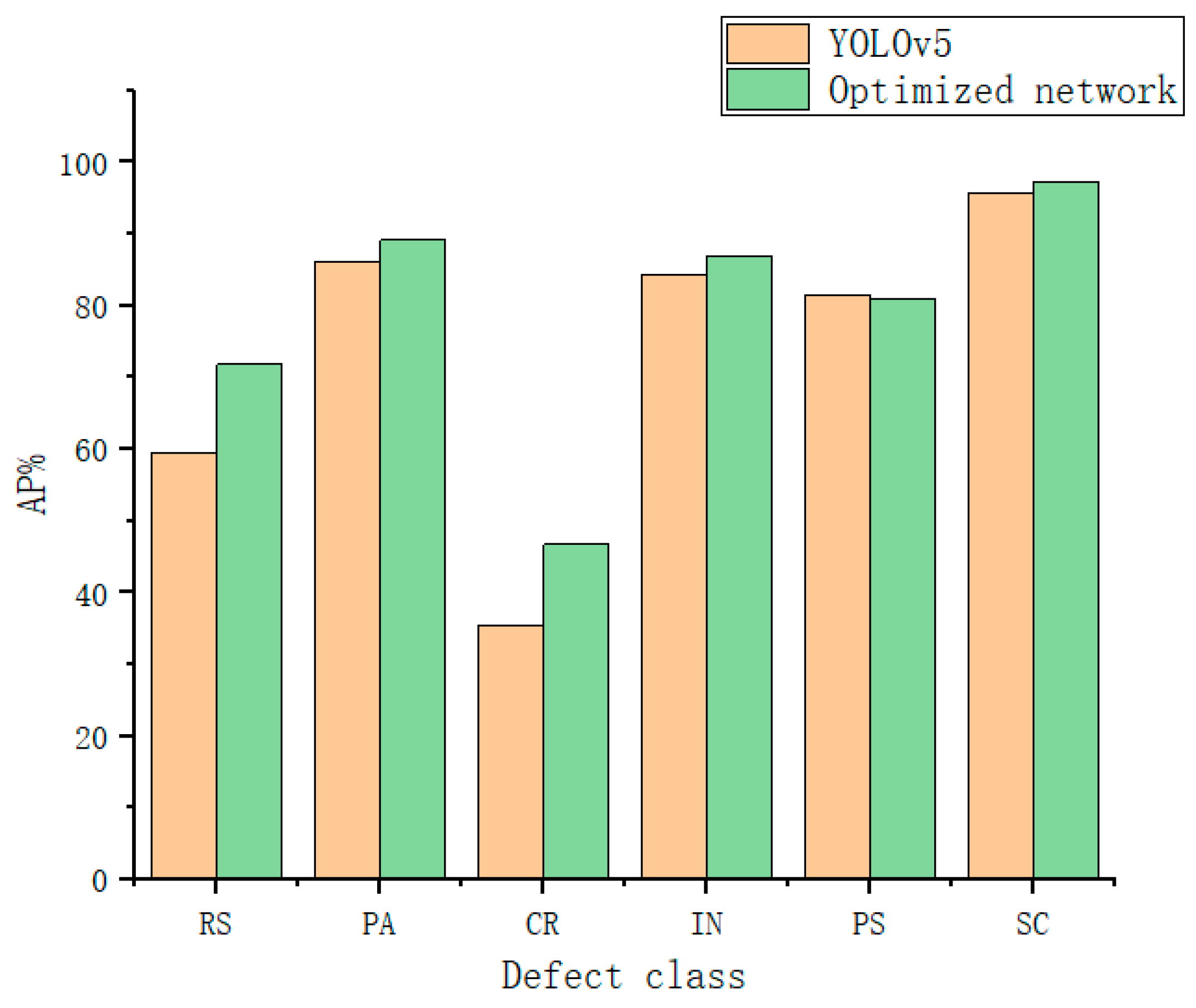
This paper uses the publicly available steel dataset from Northeastern University. Because of the random nature of the dataset, the experimental results differ in different systems. Therefore, the evaluation criteria of the improved network in this paper lie in comparing the results before and after network optimization. In this paper, we focus on optimizing the traditional YOLOv5 model. The K-means algorithm improves the anchor box; deformable convolution is introduced in the backbone module, and one C3 module is used instead of the DCnv2 module; the CBAM (convolution block attention module) attention mechanism is added to the backbone network; the Focal EIOU loss function is used instead of the CIOU loss function.

2. The Improved YOLOv5 Algorithm

2.1. Improving Anchor Boxes Based on K-means

The K-means algorithm is a classical algorithm that focuses on updating the cluster centers by selecting k cluster centers and iterating through multiple calculations of the distance from the target object to the cluster centers until the cluster centers no longer change.

The YOLOv5 network requires a pre-set Anchor box size for training. There are nine anchors in the YOLOv5 network, and the researcher sets the initial values empirically. In this paper, the steel defect detection varies greatly from defect to defect, and the initial Anchor box does not guarantee the detection probability. In this paper, we propose to use the K-means algorithm to re-cluster the steel dataset to obtain the Anchor box parameters that are more suitable for detection. The parameters of the obtained Anchor box are similar to the size of the steel defects in this paper, which can increase the percentage of target defect pixels and make the target feature extraction more effective while balancing positive and negative samples, thus improving the training speed and recognition rate of the network.

The K-means clustering algorithm has a Euclidean distance calculation between samples and cluster centers. Nevertheless, this calculation cannot measure the degree of overlap between two rectangular boxes; this paper uses 1 − IOU to replace the original Euclidean distance, as shown in Formula (1).

$$\begin{array}{c}{d}_{\left(box,center\right)}=1-{IOU}_{\left(box,center\right)}\end{array}$$

(1)

where $d_{\left(box,center\right)}$ denotes the distance from the target box to the cluster center, and ${IOU}_{\left(box,center\right)}$ denotes the overlap degree between the target box and the cluster center, i.e., the ratio of the intersection of the two boxes to the concatenation; the value of IOU is taken between 0 and 1. When the two boxes are closer, the value of IOU is larger, and the value of d is smaller, i.e., the value of d is inversely proportional to the value of IOU. The relationship between the two is reflected in Equation (1). The specific steps of the K-means algorithm are as follows:

• Initialize K cluster centers; K is taken as 9 in this paper.
• Use the similarity measure, which generally uses Euclidean distance; this paper uses Equation (1) instead of calculating the Euclidean distance. Assign each sample to the cluster center with the closest distance to it.
• Calculate the mean value of all samples in each cluster and update the cluster center.
• Repeat steps 2 and 3 until the cluster centers no longer change or the maximum number of iterations is reached.

The above operation obtained the nine Anchor box parameters suitable for this paper. The Anchor box parameters were as follows: (18,35), (23,76), (31,23), (45,42), (58,74), (70,153), (125,90), (135,51), and (165,192).

2.2. Deformable Convolution

The convolutional kernel samples the input feature map at a fixed location, the pooling layer continuously reduces the size of the feature map, and the ROI pooling layer generates spatially location-constrained ROI. Therefore, when the convolutional kernel weight is fixed, it results in the same CNN processing different regions of a map with the same perceptual field size, which is unreasonable for convolutional neural networks. The convolutional layer must automatically adjust the scale or perceptual field when different locations have different scales.

The steel defect detection in this paper has six different defects, and the target defects have irregular shapes. Therefore, it is more desirable that the sampling points of the convolution kernel in the input feature map are focused on the region or target of interest. The standard convolution kernel has difficulty handling such a problem. To improve the feature extraction capability of the model, deformable convolution is introduced into the backbone network [22,23,24].

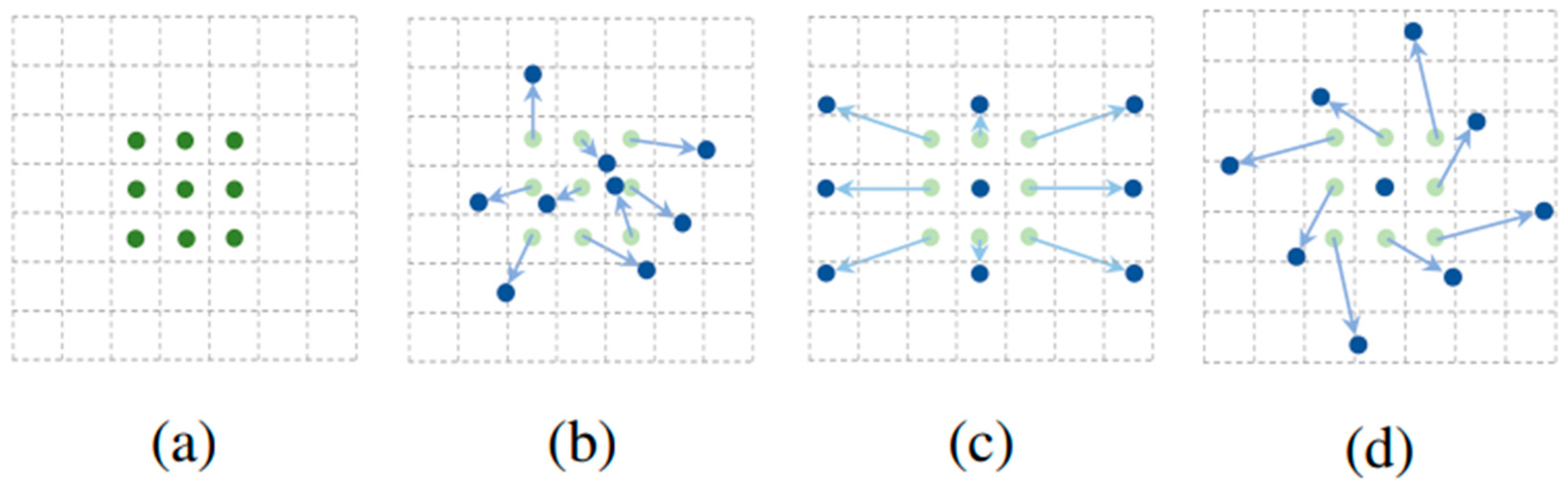
The deformable convolution operation does not change the computational operation of the convolution but adds a learnable parameter to the area of action of the convolution operation. The ordinary convolution and deformable convolution sampling points [23] are shown in Figure 1. Figure 1 was derived from [23].

The above figure shows that deformable convolution actually adds an offset to the standard convolution, which will make the convolution kernel extend to a large range during training. The deformable convolution promotes operations such as scale, aspect ratio, and rotation. Taking a 3 × 3 convolution as an example, refer to Formulas (2)–(4).

$$R=\left\{\left(-1,-1\right),\left(-\mathrm{1,0}\right),\cdots \left(\mathrm{0,1}\right),\left(\mathrm{1,1}\right)\right\}$$

(2)

$$y\left(p_0\right)=\sum _{p_n}w\left(p_n\right)·x\left(p_0+p_n\right)$$

(3)

$$y\left(p_0\right)=\sum _{p_n}w\left(p_n\right)·x\left(p_0+p_n+∆p_n\right)$$

(4)

where R defines the perceptual field of the standard convolution, $p_n$ is the n-th point in the sampled grid, and $w\left(p_n\right)$ is the corresponding convolution kernel weight factor. Each output y is sampled at nine locations, and the standard convolutional output is shown in Equation (3). Deformable convolution is the addition of an offset $∆p_n$ to the standard convolution, as shown in Equation (4). By increasing the offset, the standard convolution becomes an irregular convolution.

The principle of deformable convolution [23] is shown in Figure 2. Figure 2 was derived from [23]. The input feature map is passed through a convolution layer to obtain the deviations, and the generated channels have a dimension of 2N, corresponding to the deviations in the X- and Y-directions. There are two convolution kernels, a conventional convolution kernel for extracting features on the input image and a convolution kernel for generating deviations, which is used to learn the deformable offsets.

The process is as follows: on the basis of the input image, the feature map is extracted using a conventional convolutional kernel; the obtained feature map is used as input, and another convolutional layer is applied to obtain the deformation offset of the deformable convolution with a 2N offset layer corresponding to the amount of change in X and Y. During training, the two convolutional kernels used to generate the feature maps and to generate the offsets are learned simultaneously. The offsets are learned by back-propagation using an interpolation algorithm.

As can be seen from the above figure, in the input feature map, the normal convolution operation corresponds to a convolution sampling area of a square of convolution kernel size (green box), and the sampling area corresponding to variable convolution is the area where the blue box is located. When the shape of the detection target is irregular, such as the steel defect detection in this paper, using deformable convolution can extract better feature information.

In this paper, the deformable convolution module DCnv2 is added to the backbone module to replace one of the Conv modules, as shown in Figure 7. In this paper, we experimented with the number of DCnv2 modules. We found that using two or three DCnv2 modules to replace the traditional Conv module would increase the running time by two to three times. There was no significant improvement in the accuracy of defect detection. Therefore, in this paper, using one DCnv2 module not only did not increase the training time of the model but also improved the training accuracy of the model.

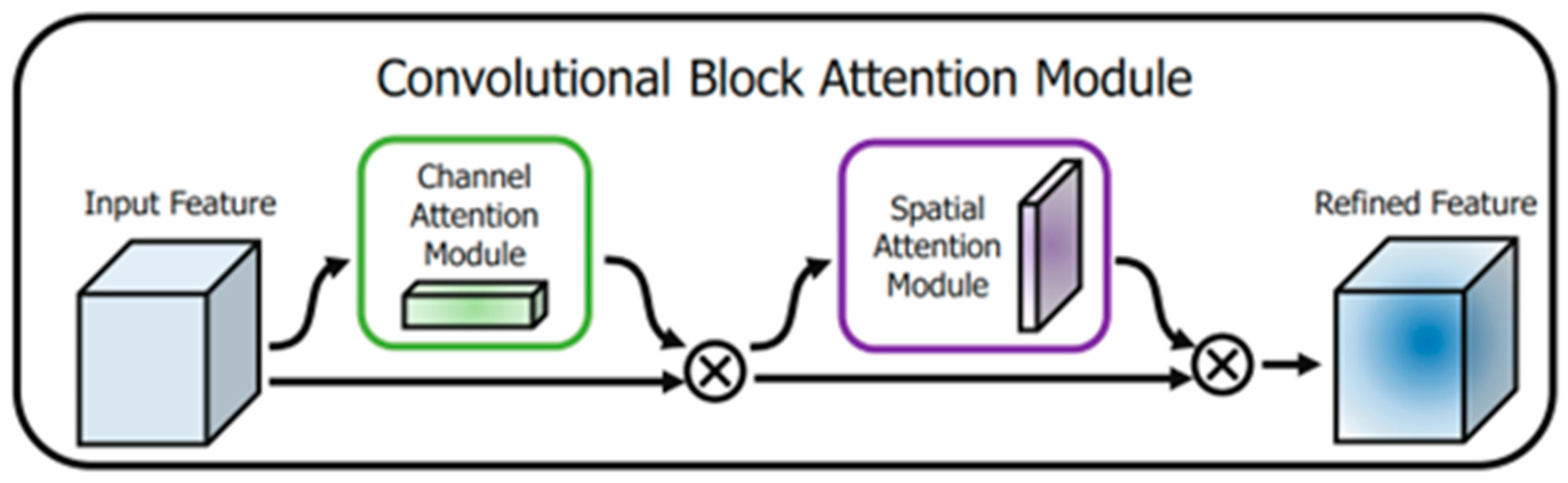
2.3. CBAM Attention Mechanism

In computer vision, the added attention mechanism enables different parts of an image or feature map to be weighted differently. This allows the network to focus on different regions of the feature map to another degree, allowing the network to focus better on the target region of interest. The attention mechanism can enhance the information extraction from the image and improve the focus on the detection target.

Due to the low pixels of the images of the steel dataset in this paper, some defects are difficult to detect. In this paper, an attention mechanism is added to the network to improve the detection probability of the network. The common attention mechanisms are CBAM, CA, SE, ECA, and SimAM, and this paper experimented with each of the above five attention mechanisms. Comparing the effects of the five attention mechanisms, we found that CBAM had the best effect, followed by the SE module; the other three attention mechanisms had relatively poor effects. Therefore, this paper chose to use the CBAM attention mechanism.

The CBAM attention mechanism consists of channel and spatial attention mechanisms [25]. Figure 3 was derived from [25]. As shown in Figure 3, CBAM is a simple and effective attention module for feed-forward convolutional neural networks. Given an intermediate feature map, the module infers attention weights sequentially along two dimensions, channel and spatial, and then multiplies them with the input feature map for adaptive feature modification. CBAM is a lightweight module with low computational effort and can be integrated anywhere in the network.

The channel attention module shown in Figure 4 was derived from [25]. The input feature maps F (H × W × C) are subjected to maximum global pooling and global average pooling to obtain two 1 × 1 × C feature maps; then, they are fed into a two-layer neural network (MLP), which is shared by both layers; then, the outputs of the feature from the MLP are summed; finally, the sigmoid activation operation is performed to generate the input needed by the spatial attention mechanism module features.

The expression for the channel attention module is shown in Equation (5).

$$\begin{array}{c}{M}_C\left(F\right)=\sigma \left(MLP\left(AvgPool\left(F\right)\right)+MLP\left(MaxPool\left(F\right)\right)\right)\\ =\sigma \left(W_1\left(W_0\left(F_{avg}^C\right)\right)+W_1\left(W_0\left(F_{max}^C\right)\right)\right)\end{array}$$

(5)

where σ is the sigmoid activation function, MLP is a simple artificial neural network, $AvgPool$ is averaging over the local range, $MaxPool$ is maximizing over the local range, $W_0$ and $W_1$ are the input weights of $MLP$, and $F_{avg}^C$ and $F_{max}^C$ denote the average pooling and maximum pooling features, respectively.

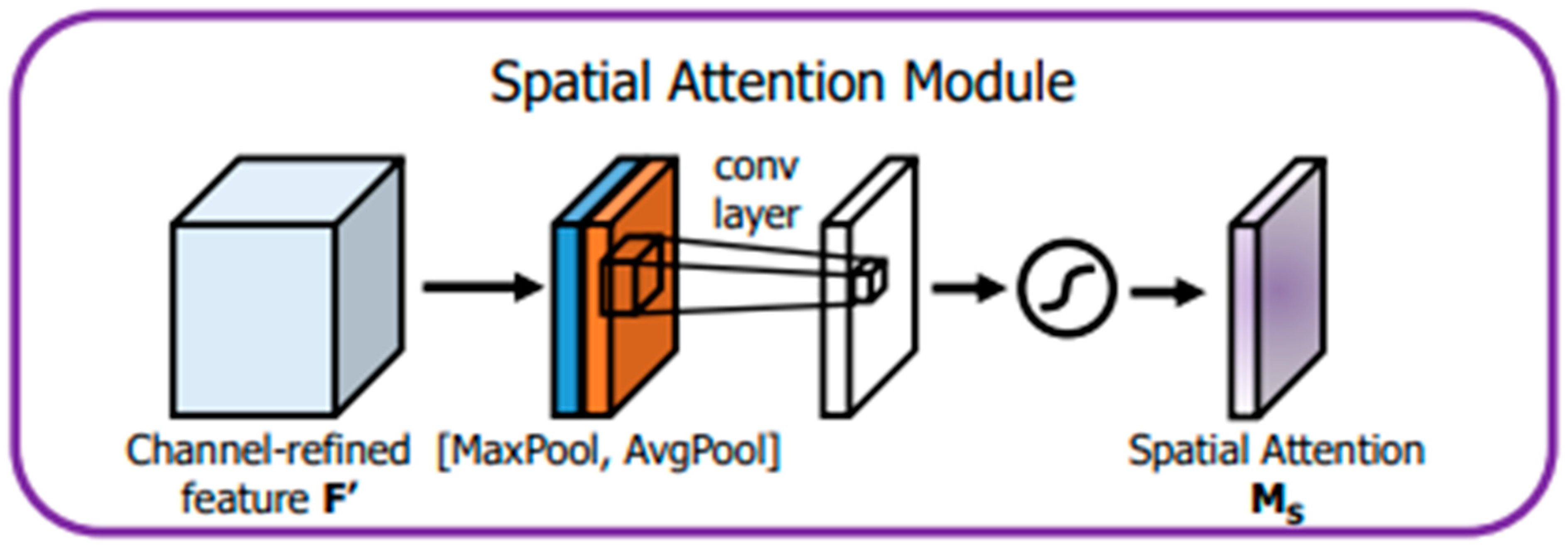
The spatial attention module shown in Figure 5 was derived from [25]. The feature map F’s output from the channel is used as the input feature map of this module. First, after maximum global pooling and global average pooling, two H × W × 1 feature maps are obtained; the two feature maps are stitched on the basis of the channels; then, after the 7 × 7 convolution operation, the dimensionality is reduced to one channel, i.e., H × W × 1; then, the spatial attention features are generated by the sigmoid activation function; the spatial attention features are multiplied with the input features of the spatial attention module, yielding the final generated features. The expression of the spatial attention module is shown in Equation (6).

$$\begin{gathered} M_S\left(F\right)=\sigma \left(f^{7\times 7}\left(\left[AvgPool\left(F\right);MaxPool\left(F\right)\right]\right)\right) \\ =\sigma \left(f^{7\times 7}\left(\left[F_{avg}^S;F_{max}^S\right]\right)\right) \end{gathered}$$

(6)

where σ is the sigmoid activation function, $f^{7\times 7}$ is the 7 × 7 convolution operation, and $F_{avg}^S$ and $F_{max}^S$ denote the average pooling and maximum pooling features, respectively.

In this paper, the CBAM attention mechanism is added to the network’s backbone network, and three CBAM modules are added after three C3 modules, as shown in Figure 7. The heat map of the attention mechanism can clearly show the state of the feature map during processing. Taking one of the defects as an example, the feature map after the image passed through the C3 module and the CBAM module is shown in Figure 6.

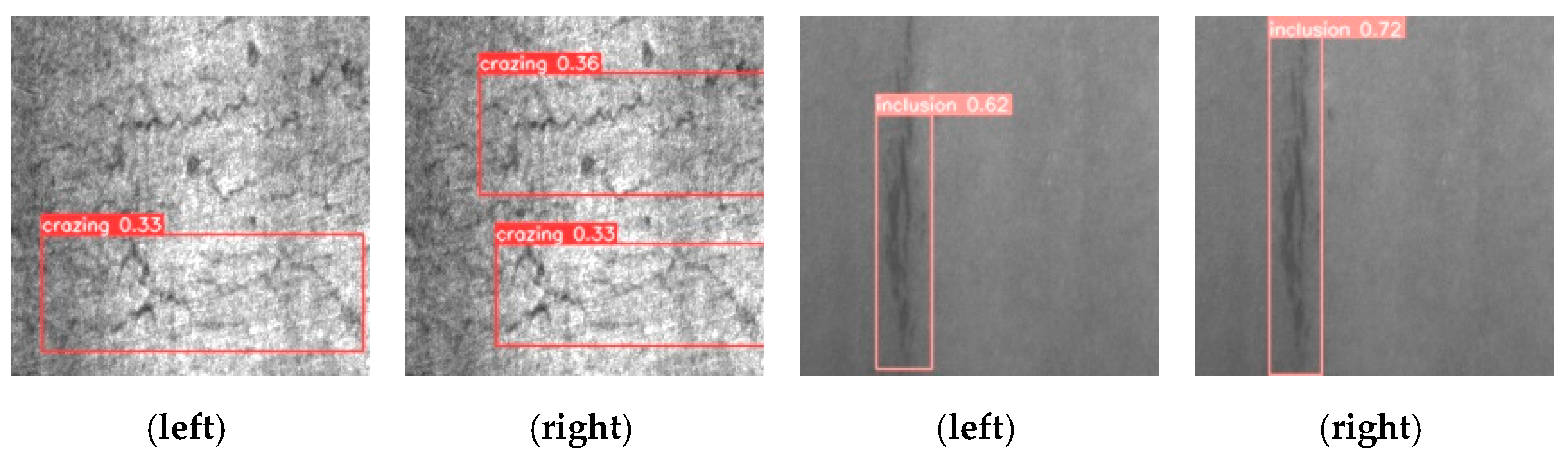
As can be seen from the above figure, after the bad image passes through the C3 module, the defective features are only recognized as a small part, which is not conducive to the subsequent feature extraction. After adding the CBAM attention mechanism, the features that can be recognized are significantly increased, which is beneficial to the subsequent information extraction. This shows that this paper effectively adds a CBAM attention mechanism to the backbone network Figure 7.

2.4. Focal EIOU

The traditional YOLOv5 uses the loss function of CIOU (complete intersection over union) for calculation, which has a greater improvement than IOU, GIOU, and DIOU (distance intersection over union). The IOU loss function performs the calculation of the intersection and merging ratio, which is the ratio of the area of the intersection area of the prediction box A and the real box B to the merging area. The CIOU loss function is expressed as Formula (7).

$$IOU=\frac{A\cap B}{A\cup B}$$

(7)

When the predicted box does not intersect with the real box, the value of IOU is 0, which causes the gradient of the loss function to vanish. The GIOU loss function is optimized for this case; the GIOU loss function obtains the minimum external rectangle C of the two rectangular boxes A and B, and characterizes the distance of the boxes by C. The GIOU formula is shown below.

$$GIOU=IOU-\frac{C-A\cup B}{C}$$

(8)

From the formula of GIOU, we know that the range of GIOU takes the value of (−1, 1). When the rectangular boxes A and B do not intersect, the farther the two boxes are, the larger C is, and the closer the GIOU is to the value of −1. When the rectangular boxes A and B completely overlap, the numerator of $1-\frac{A\cup B}{C}$ is 0, and the GIOU takes the value of 1. However, GIOU also cannot handle the case where the overlapping areas are the same, but the directions and distances are different, as shown in Figure 8.

For this situation, the researchers propose the DIOU loss function, which considers the degree of overlap between the target and the prediction frame and the centroid distance. The formula of the DIOU loss function is as follows:

$$L_{CIOU}=1-IOU+\frac{\rho \left(b^p,b^g\right)}{c^2}$$

(9)

where $b^p$ and $b^g$ denote the prediction frame and the real frame, respectively, $\rho \left(b^p,b^g\right)$ denotes the Euclidean distance between the centroids of the two rectangular frames, and c denotes the diagonal distance of the minimum external rectangle. DIOU ignores the aspect ratio problem, although it carries out some optimization. This problem is implemented in the CIOU loss function, as shown in Formula (10).

$$L_{CIOU}=1-IOU+\left(1-\frac{A\cup B}{C}+\alpha v\right)$$

(10)

The CIOU loss function is used in the YOLOv5 algorithm, which was greatly optimized compared with the previous loss function. However, although the CIOU loss function considers the overlap area, centroid distance, and aspect ratio of the bounding box regression, the aspect ratio description of the CIOU loss function is a relative value, which has some ambiguity and sometimes hinders the optimization of the model. It does not consider the balance problem of difficult and easy samples.

For the above situation, this paper adopts the EIOU (efficient intersection over union) loss function instead of the CIOU loss function and calculates the difference values of width and height using the CIOU instead of the aspect ratio; for the problem of an imbalance between difficult and easy samples, Focal loss is introduced to solve it. The Focal EIOU loss function is used in this paper, as shown in Formulas (11) and (12).

$$L_{EIOU}=L_{IOU}+L_{dis}+L_{asp}=1-IOU+\frac{{\rho }^2\left(b,b^{gt}\right)}{c^2}+\frac{{\rho }^2\left(w,w^{gt}\right)}{c_w^2}+\frac{{\rho }^2\left(h,h^{gt}\right)}{c_h^2}$$

(11)

$$L_{Focal-EIOU}={IOU}^{\gamma }{L}_{EIOU}$$

(12)

where $C_w$ and $C_h$ are the width and height of the smallest external rectangle of the two rectangular boxes, $b$ and $b^{gt}$ denote the centroids of the prediction box and the target box, $\rho$ denotes the Euclidean distance, and $\gamma$ is a parameter controlling the degree of outlier suppression.

The EIOU loss function contains three components: overlap loss, center distance loss, and width–height loss, with the first two using the CIOU approach; moreover, the real differences in target and anchor box widths and heights are considered, and the EIOU function minimizes these differences to accelerate the convergence of the model.

3. Experimental Results and Analysis

3.1. Experimental Dataset and Experimental Environment

This paper uses the NEU-DET public dataset, a steel surface defect dataset produced by Northeastern University. The dataset has six types of defects, namely, rolled-in-scale (RS), patches (PA), crazing (CR), inclusion (IN), pitted surface (PS), and scratches (SC), as shown in Figure 9a. The dataset has a total of 1800 images, with 300 images for each type of defect, and the image size is 200 × 200. In this paper, the dataset is randomly disrupted, and the training set, validation set, and test set are divided according to the ratio of 8:1:1, i.e., 1440 images for the training set, 180 images for the validation set, and 180 images for the test set. The number of bounding boxes for each class of the training set in the dataset was counted. The results are shown in Figure 9b.

3.2. Evaluation Criteria

The evaluation criteria for target detection are mainly accuracy metrics and speed metrics. The speed index is the number of images processed per second or the processing time per image under the same operating conditions; the accuracy index considers the average precision (AP) and the average precision mean (mAP). Precision (P) is the detection probability, while recall (R) is the detection completion rate, as shown in Formulas (13)–(16).

$$Precision=\frac{TP}{TP+FP}$$

(13)

$$Recall=\frac{TP}{TP+FN}$$

(14)

$${AP}_i={\int }_0^{1}P\left(R\right)d\left(R\right)$$

(15)

$$mAP=\frac{1}{N}\sum _{i=1}^N{AP}_i$$

(16)

In the formulas, $TP$ is the number of positive samples correctly identified, $FP$ is the number of negative samples incorrectly identified as positive samples, $FN$ is the number of positive samples incorrectly identified as negative samples, and N is the number of target categories.

3.3. AP Value and P–R Curve of the Optimized Network

As can be seen from Figure 10, using the improved algorithm, except for a 0.5% drop in defective PS, all other defects are improved. RS is enhanced by 12.3%, PA is improved by 3.1%, CR is improved by 11.3%, IN is improved by 2.6%, and SC is improved by 1.5%, with RS and CR improving the most. Using the P–R curves in Figure 11, we can judge the network detection performance as a function of the area enclosed by each curve and the coordinate axes. Except for CR, which has low accuracy, the detection of other defects is good, with defect SC having the highest accuracy of 97.3%. Overall, the detection probability of the optimized network is improved.

From the detection results of YOLOv5, it can be seen that the SR detection probability can reach more than 95%; however, the RS and CR detection probability is very low. It is known that this dataset has the problem of uneven sample difficulty; hence, this paper introduces the Focal loss function to mine the difficult samples. Combined with the other optimizations in this paper, the final detections of RS and CR are greatly improved.

3.4. Ablation Experiment

To visualize the performance of the modified network, ablation experiments were conducted on the modified network, and the experimental results are shown in

Table 1. Results of ablation experiments.

Method	Experiment 1	Experiment 2	Experiment 3	Experiment 4	Experiment 5
YOLOv5s	✓	✓	✓	✓	✓
DCnv2		✓	✓	✓	✓
CBAM			✓	✓	✓
Focal EIOU				✓	✓
Anchor box					✓
mAP%	74.5	75.8	77.1	77.7	78.8
Number of parameters (106)	7.02	7.67	7.72	7.72	7.72

.

In this paper, the above improvements were made using YOLOv5s, as shown by the results of the ablation experiments. Compared with experiments 1 and 2, the mAP value was improved from 74.5% to 75.8% by replacing one convolutional layer with a DCnv2 module in the backbone network, which shows that using deformable convolution can obtain a better perceptual field, improve the detection probability of defective targets, and reduce the leakage rate. Compared with Experiments 2 and 3, adding a three-layer CBAM attention mechanism to the backbone network enhanced the feature extraction ability, and the mAP value was further improved from 75.8% to 77.1%. Compared with experiments 3 and 4, using Focal EIOU instead of the CIOU loss function, the mAP was optimized using CIOU, and the mAP was improved by 0.6% compared with CIOU. Compared with experiments 4 and 5, the Anchor box parameters were optimized using the K-means algorithm, which is more favorable for feature extraction, and the mAP value was improved from 77.7% to 78.8%.

During the experiment, the position and number of DCnv2 modules were studied. If three DCnv2 modules were used, the training time was increased by a factor of two, while the training time was doubled using two DCnv2 modules; despite the increase in training time, the detection probability of the defective target did not increase. In this paper, when using one DCnv2 module and replacing the convolutional layer after the second C3 module, the training time was almost the same and the training effect was the best.

3.5. Results and Analysis

Figure 12 shows the detection results of the model before and after the improvement. It can be seen in the detection results that some of the previously undetected defects were detected in the optimized one; the detection probability of most of the previously detected defects was improved.

To verify the advantages of the improved algorithm, the results under different networks were compared using the same dataset. In this paper, we used faster R-CNN with higher detection probability, two improved faster R-CNNs, and YOLOv5s in the YOLO series as a comparison, and the results are shown in

Table 2. Performance comparison of different models.

Algorithm	mAP (%)	P (%)	R (%)	FPS (Images/Second)
Faster R-CNN (VGG)	67.8	-	-	<20
Faster R-CNN (MobileNetv2)	72.7	-	-	<20
Faster R-CNN (ResNet50 + FPN)	74.9	-	-	<20
YOLOv5s	74.5	74.9	72.5	111
Improved YOLOv5 algorithm	78.8	76.4	76.1	100

.

Since the results of the deep learning algorithm are random, the improved algorithm was trained and tested several times to verify the accuracy of the algorithm results. The effectiveness of the improved algorithm could be observed by taking the average of the experimental results. The experimental results are shown in

Table 3. Validation of experimental results.

Number of Experiments	1	2	3	4	5	6	7	8	9	10
Results (%)	78.7	78.5	78.8	77.9	78.6	78.9	78.3	78.7	78.8	78.1
Mean value of results (%)	78.53
Standard Deviation (%)	0.313

.

From the above table, the best result was 78.9%, and the worst result was 77.9%; the difference between the best and the worst was 1%, which shows that there is still some fluctuation in the network. The average result of the 10 experiments was 78.53%, the standard deviation was 0.313%, and most other results were more than 78.5% after removing the best and the worst experimental results. The experimental results were concentrated in the range between 78.7% and 78.8%. Therefore, the improvement of the network in this paper was effective.

4. Conclusions

To address the problem of low accuracy of steel surface defect detection, this paper proposed an improved YOLOv5 steel surface defect detection algorithm using the NEU-DET dataset and optimizing the traditional YOLOv5 network to improve the accuracy of steel defect detection.

Based on YOLOv5, a convolution module in the backbone network was replaced by a deformable convolution DCnv2 module, which could obtain a better perceptual field and was more conducive to obtaining information about the detection target; an attention mechanism was introduced in the backbone network, and three CBAM attention modules were added to strengthen the network’s ability to learn features; the CIOU loss function was replaced by a Focal EIOU loss function; lastly, the K-means algorithm was used to re-cluster the dataset in this paper to obtain more suitable Anchor box parameters.

The optimized method in this paper achieved an mAP value of 78.8% in the NEU-DET dataset, which was 4.3% higher than before optimization, and the inference time per image was only increased by 1 ms. However, the detection probability for crazing defects was still not high; thus, the next step will be to continue to improve the detection probability of the model for crazing defects and further improve the detection probability of steel surface defects.